Universality classes and crossover scaling of Barkhausen noise in thin films

Abstract

We study the dynamics of head-to-head domain walls separating in-plane domains in a disordered ferromagnetic thin film. The competition between the domain wall surface tension and dipolar interactions induces a crossover between a rough domain wall phase at short length-scales and a large-scale phase where the walls display a zigzag morphology. The two phases are characterized by different critical exponents for Barkhausen avalanche dynamics that are in quantitative agreement with experimental measurements on MnAs thin films.

When subject to an external magnetic field, a ferromagnetic material shows a sequence of discrete and intermittent jumps of the magnetic domain walls (DW’s), known as the Barkhausen effect DUR-06 , a paradigmatic example of crackling noise in materials SET-01 . The statistical properties of the Barkhausen noise are usually studied by measuring the size distribution $P(s)$ of such jumps, or avalanches, which typically follows a power law $P(s)\sim s^{-\tau}$, with the exponent $\tau$ characterizing the universality class of the avalanche dynamics. In three dimensional bulk ferromagnetic materials, the scaling behavior of the Barkhausen effect is understood theoretically in terms of the depinning transition of domain walls ZAP-98 with two distinct universality classes for amorphous and polycrystalline materials DUR-00 . A similar clear-cut classification does not exist in lower dimensions, despite Barkhausen avalanches having been studied experimentally for decades in several ferromagnetic thin films with in-plane WIE-77 ; WIE-78 ; PUP-00 ; KIM-03 ; SAN-06 ; RYU-07 or out-of-plane anisotropy SCH-04 ; LIE-05 . This issue is particularly important because these low-dimensional magnetic structures have become increasingly relevant for various technological applications PAR-08 ; HAY-08 .

An important step towards understanding the different universality classes in thin films was achieved by the magneto-optical experiments of Ryu et al. RYU-07 , who observed a crossover between two different avalanche size exponents $\tau$ as temperature $T$ was varied close to but below the Curie temperature $T_{c}$ of a 50 nm MnAs film. This crossover was accompanied by changes in DW morphology, such that the DW structure evolves from rough for high $T$ to DW’s with a pronounced tendency to form zigzag or sawtooth -like patterns for lower $T$. It was argued that by varying $T$ close to $T_{c}$, one can tune the value of the squared saturation magnetization $M_{s}^{2}$, and thus the strength of the long-range dipolar interactions between different DW segments. The zigzag pattern is expected to arise as a result of a competition between the domain wall energy and the dipolar interactions, with the former favoring a flat horizontal DW, while the latter would prefer a vertically spread DW to reduce the magnetic charge density MUG-10 ; CER-06 ; CER-07 .

In this Letter, we provide a theoretical explanation for the experimentally observed universality classes and the crossover between them. Due to the essentially $2d$ thin film geometry considered here (the film thickness $\Delta_{z}$ is much smaller than the DW length), we model the DW as a flexible line $\Sigma$ with surface tension $\gamma_{w}$ due to DW energy. The line moves within the $xy$ plane, and has an average orientation along the $x$ axis. It is taken to separate two magnetic domains with magnetization along $\pm\hat{{\bf y}}$, respectively. Thus, a head-to-head DW is characterized by a magnetic charge density $\sigma({\bf r})=2M_{s}\cos\theta({\bf r})$ along the DW, with $\theta({\bf r})$ the angle between the local DW normal $\hat{\bf n}$ and the $\hat{{\bf y}}$ direction. These magnetic charges then lead to a magnetostatic field ${\bf H}_{m}({\bf r})=\int_{\Sigma^{\prime}}\sigma({\bf r^{\prime}})({\bf r}-{\bf r^{\prime}})/|{\bf r}-{\bf r^{\prime}}|^{3}ds^{\prime}$, the $y$ component of which is acting on the DW segments, along with an applied field ${\bf H}_{a}=H_{a}\hat{\bf{y}}$. In addition, the DW segments interact with quenched disorder, described by a random pressure field ${\bf\eta}({\bf r})$ due to short range interactions with random pinning centers. Thus, the total normal pressure difference $\Delta p$ acting across the DW at point ${\bf r}$ reads

$$\Delta p({\bf r}) = \gamma_{w}/R({\bf r})+2M_{s}\mu_{0}H_{a}+{\bf\eta}({\bf r})\cdot\hat{\bf n}+$$

$$+4\mu_{0}M_{s}^{2}\int_{\Sigma({\bf r}^{\prime})}\frac{(y-y^{\prime})\cos\theta^{\prime}}{[(x-x^{\prime})^{2}+(y-y^{\prime})^{2}]^{3/2}}ds^{\prime},$$

where $R({\bf r})$ is the local radius of curvature. To simulate such a system, we discretize the DW along the $x$ direction, by using the film thickness $\Delta_{z}$ as the lattice constant, and describe the DW by a single-valued function $y=h(x,t)$, with $x=i=1,2,\dots,L$. The local DW velocity is assumed to be proportional to the local pressure acting on the DW, such that the equation of motion for the DW line segment $i$ along the $y$ direction is given by

$$\Gamma\frac{\partial h_{i}}{\partial t} = \frac{1}{\cos\theta_{i}}\bigg{[}\gamma_{w}\frac{\partial^{2}h_{i}}{\partial x^{2}}+2M_{s}\mu_{0}H_{a}+\eta(i,h_{i})+$$

$$+4\mu_{0}M_{s}^{2}\Delta_{z}^{2}\sum_{j\neq i}\frac{h_{i}-h_{j}}{[\Delta_{z}^{2}(i-j)^{2}+(h_{i}-h_{j})^{2}]^{3/2}}\bigg{]},$$

where we have approximated the curvature term by a discretized Laplacian, $\theta_{i}$ is the angle between the normal of the $i$th segment and the $y$ direction, and $\Gamma$ is a damping constant. The factor $1/\cos\theta_{i}$ multiplying the right hand side of Eq. (Universality classes and crossover scaling of Barkhausen noise in thin films) transforms normal motion into motion along the $y$ direction. The quenched random force has correlations $\langle\eta(i,h_{i})\eta(j,h_{j})\rangle=\sigma^{2}\delta(i-j)\delta(h_{i}-h_{j})$. We further write Eq. (Universality classes and crossover scaling of Barkhausen noise in thin films) in non-dimensional units, by measuring lengths in units of $\Delta_{z}$ and times in units of $\Gamma\Delta_{z}/(\mu_{0}M_{s}^{2})$. The resulting dimensionless equation of motion reads

$$\frac{\partial h_{i}}{\partial t} = \frac{1}{\cos\theta_{i}}\bigg{[}\lambda\frac{\partial^{2}{h}_{i}}{\partial{x}^{2}}+{F}_{ext}+{\eta}(i,{h}_{i})+$$

$$+4\sum_{j\neq i}\frac{{h}_{i}-{h}_{j}}{[(i-j)^{2}+({h}_{i}-{h}_{j})^{2}]^{3/2}}\bigg{]},$$

where the dimensionless driving force is ${F}_{ext}=2H_{a}/M_{s}$ and $\lambda\equiv l_{D}/\Delta_{z}$ is the ratio between the “domain formation” length BER-98 $l_{D}=\gamma_{w}/(\mu_{0}M_{s}^{2})$ and the film thickness. In dimensionless units, the quenched random force has correlations $\langle{\eta}(i,{h}_{i}){\eta}(j,{h}_{j})\rangle={\sigma}^{2}\delta(i-j)\delta({h}_{i}-{h}_{j})$, with ${\sigma}=\sigma/(\mu_{0}M_{s}^{2}\Delta_{z})$. Periodic boundary conditions are implemented by using the nearest image approximation to compute the non-local dipolar forces.

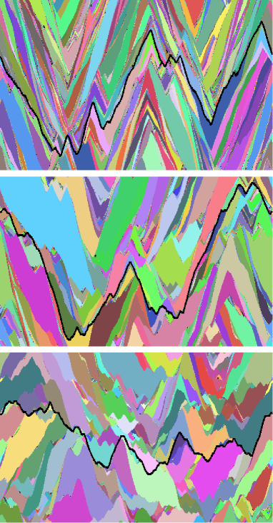
Figure 1: (color online) The spatial structure of Barkhausen avalanches for $\lambda=1$ (top), $\lambda=2$ (middle) and $\lambda=4$ (bottom). The domain wall is moving from top to bottom, and the area swept over by each avalanche has been colored with a random color. An example of the DW structure is given by a black line in each case.

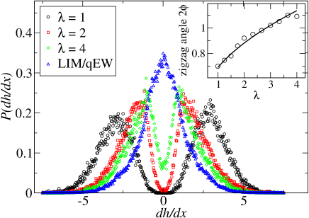
Figure 2: (color online) Distributions of the local slopes $dh/dx$ (see text for definition) for various $\lambda$. The inset shows the corresponding zigzag angle $2\phi$ as a function of $\lambda$. The solid line is a fit to of Eq. (5), corresponding to ${l}=3.9$.

To mimic the experiments of Ref. RYU-07 , we simulate the system by integrating Eq. (Universality classes and crossover scaling of Barkhausen noise in thin films) numerically, fixing the external force ${F}_{ext}$ to a constant value below the critical depinning force ${F}_{c}$, and monitor the dynamics of the DW. Whenever the average DW velocity $V(t)=1/L\sum_{i}\partial{h}_{i}/\partial{t}$ falls below a low threshold value $V_{th}$, a randomly selected DW segment is given a “kick”, such that an additional local force acting on the DW segment is first increased linearly from zero until $V>V_{th}$, and then decreased continuously back to zero. This can then trigger an avalanche, which lasts until the average velocity of the front again falls below $V_{th}$, and the process is repeated. The area (measured in units of $\Delta_{z}^{2}$) over which the DW moves between two such triggering events (which mimic the effect of thermal activation) is taken to be the avalanche size ${s}$. Fig. 1 shows the spatial structure of the avalanches for different $\lambda$-values. For small $\lambda$, the DW’s exhibits a clear zigzag morphology (with avalanches tilted accordingly), and roughen due to disorder as $\lambda$ is increased.

We further characterize the zigzag morphology by considering the distributions of the local slopes $\partial{h}/\partial{x}$ of the DW, see Fig. 2. For finite $\lambda$, the distributions are bimodal, reflecting the fact that the dipolar interactions render the flat DW unstable. For the sake of comparison, we show also the slope distribution for the Linear Interface Model (LIM)/quenched Edwards-Wilkinson (qEW) equation (i.e. Eq. (Universality classes and crossover scaling of Barkhausen noise in thin films) without the non-local term, corresponding to the limit $\lambda\rightarrow\infty$), displaying a single peak at $\partial{h}/\partial{x}=0$. The inset of Fig. 2 shows the zigzag angle $2\phi$, defined as $2\phi=2\tan^{-1}(1/\langle|\partial{h}/\partial{x}|\rangle)$. For small $\lambda\sim 1/M_{s}^{2}$, $2\phi$ is linear in $\lambda$, similarly to experimental results RYU-06 , while for very large $\lambda$ the DW becomes rough, and the concept of the zigzag angle is ill-defined. An approximate analytical estimate of the $\lambda$-dependence of $2\phi$ can be obtained by requiring balance between forces due to line tension and dipolar interactions. The former can be estimated as $\lambda\partial^{2}{h}/\partial{x}^{2}=\lambda 2m/{l}$, where $m=\langle|\partial{h}/\partial{x}|\rangle$ is the magnitude of the zigzag slope, and ${l}$ is the length of the “transition region” at the tip of the zigzag where a constant curvature $2m/{l}$ is assumed. These have to be balanced by forces due to dipolar interactions, which we write in terms of the slope $m$ as

$$4\sum_{j\neq i}\frac{m|i-j|}{|i-j|^{3}(1+m^{2})^{3/2}}=4\frac{m}{(1+m^{2})^{3/2}}2\zeta(2),$$ (4)

where $\zeta(2)=\pi^{2}/6$. Thus, from the force balance condition, one obtains for the slope $m=\sqrt{(2\pi^{2}l/3\lambda)^{2/3}-1}$, corresponding to the zigzag angle

$$2\phi=2\tan^{-1}(m^{-1})=2\tan^{-1}[(2\pi^{2}l/3\lambda)^{2/3}-1]^{-1/2}.$$ (5)

A good fit to the data with Eq. (5) can be obtained by using ${l}$ as a fitting parameter, resulting in ${l}\approx 3.9$, see the inset of Fig. 2.

For small $\lambda$, the statistical properties of the Barkhausen avalanches are expected to reflect the dominant nature of the dipolar interactions. Fig. 3 shows the avalanche size distributions $P({s})$ for $\lambda=1$ and various ${F}_{ext}<{F}_{c}$. The distributions are found to obey

$$P({s})={s}^{-\tau_{DIP}}\mathcal{F}_{DIP}\left[\frac{{s}}{({F}_{c}-{F}_{ext})^{-1/\sigma_{DIP}}}\right],$$ (6)

where $\mathcal{F}_{DIP}(x)$ is a scaling function, $\tau_{DIP}\simeq 1.33$ and $1/\sigma_{DIP}\simeq 3.5$. The value of $\tau_{DIP}$ characterizes the “zigzag” universality class dominated by dipolar interactions, and is close to that found for certain other systems with long-range anisotropic interaction kernels, such as models of amorphous plasticity TAL-11 . For larger $\lambda$, while large enough avalanches are still dominated by the dipolar interactions, small avalanches start to be governed by the surface tension, and the power law part of Eq. (6) has to be replaced by a crossover scaling form including two different power laws with the corresponding $\tau$-exponents,

$$P({s})={s}^{-\tau_{LIM}}[1+({s}/{s}_{\chi})^{(\tau_{DIP}-\tau_{LIM})k}]^{-1/k}\mathcal{F}({s}/{s}_{0}),$$ (7)

where ${s}_{\chi}$ is a crossover avalanche size separating the two regimes, $k$ controls the sharpness of the crossover and ${s}_{0}$ is the cut-off avalanche size. The short length scale exponent is expected to be that of the LIM/qEW, $\tau_{LIM}\simeq 1.11$ ROS-09 and $1/\sigma_{LIM}=3.0$ ZAP-98 .

To estimate the crossover scale ${L}_{\chi}$ (and the corresponding crossover avalanche size ${s}_{\chi}$) above which the dipolar forces will dominate the line tension, we consider the continuum version of Eq. (Universality classes and crossover scaling of Barkhausen noise in thin films) for small deformation of the DW without disorder and external force,

$$\frac{\partial{h}}{\partial{t}}=\lambda\frac{\partial^{2}{h}}{\partial{x}^{2}}+4\int\frac{{h}({x})-{h}({x}^{\prime})}{|{x}-{x}^{\prime}|^{3}}d{x}^{\prime},$$ (8)

and examine the stability of a flat DW. By writing the two interaction terms in Eq. (8) in terms of their Fourier transforms, $\lambda\frac{\partial^{2}{h}_{i}}{\partial{x}^{2}}=\int d{q}{h}_{{q}}e^{i2\pi{q}{x}}(-4\pi^{2}\lambda{q}^{2})$ and $4\int d{x}\frac{{h}({x})-{h}({x}^{\prime})}{|{x}-{x}^{\prime}|^{3}}=4\int d{q}e^{i2\pi{q}{x}}{h}_{{q}}\int d{x}^{\prime}\frac{1-e^{i2\pi{q}({x}^{\prime}-{x})}}{|{x}-{x}^{\prime}|^{3}}$, one arrives at a stability condition for the mode ${q}$, $-4\pi^{2}\lambda{q}^{2}+I({q})<0$, where $I({q})\equiv 4\int d{r}\frac{1-e^{i2\pi{q}{r}}}{|{r}|^{3}}$. We expand $I({q})$ for small ${q}$, such that $I({q})\simeq 4\int_{1}^{1/{q}}d{r}({q}{r})^{2}/|{r}|\textthreesuperior=-8\pi^{2}{q}^{2}\log({q})$. Thus, the stability condition becomes $2\log({q})+\lambda>0$, which leads to a crossover length

$${L}_{\chi}=e^{\lambda/2}.$$ (9)

The crossover avalanche size is expected to scale as ${s}_{\chi}\sim{L}_{\chi}^{1+\zeta_{\chi}}$, where $\zeta_{\chi}$ is the roughness exponent of the avalanches at the crossover scale. Thus, also the crossover avalanche size is an exponential in $\lambda$,

$${s}_{\chi}=e^{(1+\zeta_{\chi})\lambda/2}.$$ (10)

Notice that this form is different from the one employed in Ref. RYU-07 .

To test this argument, we simulate the model for various $\lambda\geq 1$, and estimate ${s}_{\chi}(\lambda)$ by fitting Eq. (7) to the data. We found that $\mathcal{F}(x)=\exp(-x)$, $k=10$ (corresponding to a sharp crossover), and $\tau_{LIM}=1.11$ and $\tau_{DIP}=1.33$ produce a very good fit, see Fig. 4. Fig. 5 (a) shows the resulting ${s}_{\chi}(\lambda)$-data, which can be well fitted by an exponential, thus confirming the functional form in Eq. (10). Fig. 4 shows the avalanche size distributions for different $\lambda$, with ${s}$ rescaled with the corresponding ${s}_{\chi}(\lambda)$ and $P(s)$ by the factors $C(\lambda)$, chosen to make the different distributions overlap. This procedure reveals a clear crossover scaling, with the exponents $\tau_{LIM}\simeq 1.11$ and $\tau_{DIP}\simeq 1.33$ below and above ${s}/{s}_{\chi}=1$, respectively. Notice also that the crossover is rather sharp, taking place within one order of magnitude in ${s}/{s}_{\chi}$. This is in contrast to the results of Ref. RYU-07 , where a large crossover region with a slowly changing effective exponent was found, by using an expression for the crossover avalanche size which is different from the one found here. The crossover can also be seen by fitting a single power law with an exponential cutoff,

$$P(s)=s^{-\tau_{eff}(\lambda)}\exp\left(-\frac{{s}}{{s}_{0}(\lambda)}\right),$$ (11)

to the data. The resulting effective exponent $\tau_{eff}$ as a function of $\lambda$ is shown in Fig. 5 (b), showing again a crossover between the values of $\tau_{LIM}=1.11$ and $\tau_{DIP}=1.33$.

Figure 3: (color online) The distribution of avalanche sizes ${s}$ with $\lambda=1$, corresponding to the limit dominated by dipolar interactions, for various $F_{ext}\leq F_{c}$. The inset shows a collapse with exponents $\tau_{DIP}=1.33$ and $1/\sigma_{DIP}=3.5$.

Figure 4: (color online) The rescaled avalanche size distributions for various $\lambda$, with $F$ slightly below $F_{c}$ in each case, showing the crossover between the two scaling exponents, $\tau_{LIM}=1.11$ (dashed blue line) and $\tau_{DIP}=1.33$ (dash-dotted red line). The solid lines are fits of Eq. (7 to the data. The dependence of the crossover avalanche size $s_{\chi}$ on $\lambda$ resulting from the fits is reported in Fig. 5 (a).)

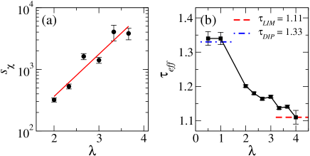
Figure 5: (color online) (a) shows the exponential dependence of the crossover avalanche size ${s}_{\chi}$ on $\lambda$. The solid line corresponds to an exponential fit ${s}_{\chi}=Ae^{B\lambda}$, with $A=15.5$ and $B=1.577$. (b) shows the effective exponent $\tau_{eff}$ as obtained by fitting Eq. (11) to the data.

To summarize, we have presented a theoretical analysis and a numerical model of DW morphology and avalanche dynamics in thin films with in-plane uniaxial anisotropy, giving rise to charged head-to-head (or tail-to-tail) DW’s. As a result of the competition between DW surface tension and dipolar interactions, the DW’s develop a zigzag structure. The avalanche dynamics displays a sharp crossover between two universality classes, characterized by the exponents $\tau_{LIM}\simeq 1.11$ and $\tau_{DIP}\simeq 1.33$, for scales dominated by the line tension and dipolar interactions, respectively. These two scaling regimes are separated by a crossover avalanche size $s_{\chi}$ which exhibits an exponential dependence on $\lambda\sim 1/M_{s}^{2}$. It is worth noticing that the dipolar interactions scale as ${q}^{2}\log({q})$ in Fourier space. Hence, in the $q\rightarrow 0$ limit, the kernel is similar to a negative surface tension, and it is therefore not possible to infer the dipolar universality class based on simple power counting (as claimed e.g. in RYU-07 ). It would instead be necessary to perform a functional renormalization group calculation along the lines of Refs. NAT-92 ; NAR-93 ; LES-97 ; ERT-94 ; CHA-00 ; LED-02 , taking into account explicitly the non-convex nature of the interaction kernel, leading to a violation of the no-passing rule usually obeyed by depinning interfaces MID-92 .

Acknowledgments. Claudio Serpico, Adil Mughal, James P. Sethna and Mikko Alava are thanked for interesting discussions. LL acknowledges the financial support of the Academy of Finland through a Postdoctoral Researcher’s Project (no. 139132) and via the Centres of Excellence Program (no. 251748), as well as the computational resources provided by the Aalto Science-IT project. SZ is supported by the European Research Council, AdG2001-SIZEFFECTS and thanks the visiting professor program of Aalto University.

References

- (1) G. Durin and S. Zapperi, The Barkhausen effect in The Science of Hysteresis, edited by G. Bertotti and I. Mayergoyz, vol. II pp 181-267 (Academic Press, Amsterdam, 2006).
- (2) J. P. Sethna, K. A. Dahmen, and C. R. Myers, Nature 410, 242 (2001).
- (3) S. Zapperi, P. Cizeau, G. Durin, and H. E. Stanley, Phys. Rev. B 58, 6563 (1998).
- (4) G. Durin and S. Zapperi, Phys. Rev. Lett. 84, 4705 (2000).
- (5) N. J. Wiegman, Appl. Phys. 12, 157 (1977).
- (6) N. J. Wiegman and R. Stege, Appl. Phys. 16, 167 (1978).
- (7) E. Puppin, Phys. Rev. Lett., 84, 5415 (2000).
- (8) D.-H. Kim, S.-B. Choe, and S.-C. Shin, Phys. Rev. Lett., 90, 087203 (2003).
- (9) L. Santi, F. Bohn, A. D. C. Viegas, G. Durin, A. Magni,R. Bonin, S. Zapperi and R. L. Sommer, Physica B 384, 144 (2006).
- (10) K.-S. Ryu, H. Akinaga, and S.-C. Shin, Nature Physics 3, 547 (2007).
- (11) A. Schwarz, M. Liebmann, U. Kaiser, R. Wiesendanger, T. W. Noh, and D. W. Kim, Phys. Rev. Lett. 92, 077206 (2004).
- (12) M. Liebmann, A. Schwarz, U. Kaiser, R.Wiesendanger, D.-W. Kim, and T.-W. Noh, Phys. Rev. B 71, 104431 (2005).
- (13) S. S. P. Parkin, M. Hayashi, and L. Thomas, Science 320, 190 (2008).
- (14) M. Hayashi, L. Thomas, R. Moriya, C. Rettner, and S. P. Parkin, Science 320, 209 (2008).
- (15) A. Mughal, L. Laurson, G. Durin, and S. Zapperi, IEEE Trans. Magn. 46, 228 (2010).
- (16) B. Cerruti and S. Zapperi, J. Stat. Mech. P08020 (2006).
- (17) B. Cerruti and S. Zapperi, Phys. Rev. B 75, 064416 (2007).
- (18) G. Bertotti, Hysteresis in Magnetism (Academic Press, Boston, 1998).
- (19) K.-S. Ryu, S.-C. Shin, H. Akinaga, and T. Manago, Appl. Phys. Lett. 88, 122509 (2006).
- (20) M. Talamali, V. Petäjä, D. Vandembroucq, and S. Roux, Phys. Rev. E 84, 016115 (2011).
- (21) A. Rosso, P. Le Doussal, and K. J. Wiese, Phys. Rev. B 80, 144204 (2009).
- (22) T. Nattermann, S. Stepanow, L. H. Tang, and H. Leschhorn, J. Phys. II (France) 2, 1483 (1992).
- (23) O. Narayan and D. S. Fisher, Phys. Rev. B 48, 7030 (1993).
- (24) H. Leschhorn, T. Nattermann, S. Stepanow, and L. H. Tang, Ann. Physik 6, 1 (1997).
- (25) D. Ertas and M. Kardar, Phys. Rev. E 49, R2532 (1994).
- (26) P. Chauve, T. Giamarchi, and P. Le Doussal Phys. Rev. B 62, 6241-6267 (2000)
- (27) P. Le Doussal, K. J. Wiese, and P. Chauve Phys. Rev. B 66, 174201 (2002)
- (28) A. A. Middleton, Phys. Rev. Lett. 68, 670 (1992).