Local Bubble. Extinction within 55 pc?

Abstract

In the mapping of the local ISM it is of some interest to know where the first indications of the boundary of the Local Bubble can be measured. The Hipparcos distances combined to $B-V$ photometry and some sort of spectral classification permit mapping of the spatial extinction distribution. Photometry is available for almost the complete Hipparcos sample and Michigan Classification is available for brighter stars south of $\delta$ = +5 (1900). For the northern and fainter stars spectral types, e.g. the HD types, are given but a luminosity class is often missing. The $B-V$ photometry and the parallax do, however, permit a dwarf/giant separation due to the value of the slope of the reddening vector compared to the gradient of the main sequence in a color magnitude diagram, in the form: $B-V$ $vs.$ $M_{V}+A_{V}$ = $V+5(1+log(\pi))$, together with the rather shallow extinction present in the Hipparcos sample. We present the distribution of median $A_{V}(l,b)$ for stars with Hipparcos 2 distances less than 55 pc. The northern part of the first and second quadrant has most extinction, up to $\sim$0.2 mag and the southern part of the third and fourth quadrant the slightest extinction, $\sim$0.05 mag. The boundary of the extinction minimum appears rather coherent on an angular resolution of a few degrees

1 Introduction

A debate on the existence of non negligible amounts of material in the local interstellar medium has taken place over several decades. The problem may be looked upon under very different angles but could perhaps be reduced to: is any matter present and if so how much and how is it distributed? The local medium has observational as well as theoretical attractions. The distribution of the cooler, dense material has consequences for the theoretical models as well as for the understanding of the propagation of the energetic radiation. The concept of the solar vicinity has condensed to be apprehended as a local low density cavity in the ISM: the Local Bubble (or as a system of interconnected bubbles). A natural question is consequently how big this local bubble or low density cavity is?

In minor photometric surveys, often for other purposes than LB studies, wall-like structures were sometimes seen: abrupt changes of the color excess over very small distances. de Geus, de Zeeuw and Lub (1989) and Knude (1987) are examples showing an onset of reddening at $\approx$100 pc in the general direction of Scorpius. Reis et al’ (2011) is a more recent example where $uvby\beta$ data has been used to outline LB.

In order to indicate the size of the LB some of the parameters characterising it must be known. The confinement of the bubble is encountered when one or more of these parameters are changed in a significant way. Such a parameter could be $n_{H}$ or the average line of sight reddening/extinction, Abt (2011), Frisch, Redfield and Slavin (2011). For the size Abt quotes the range 50-100 pc and Frisch, Redfield and Slavin present in the their Fig.  4 a sky map for stars between 50 and 100 pc displaying a nice coherent contour $E_{B-V}$ $\approx$ 0.1 mag confining a low density region. The origin of the color excesses used for this map is, however not given in any detail. In the cavity the parameters are found in certain defining ranges, typically low density and small extinction. The location where either of these defining parameters displays a rise could naively indicate the boundary of the LB. Vergely et al. (2010) and Lallement, Vergely, Valette et al. (2013) used the gradient $dE_{B-V}/dr$ = 0.0002 mag pc^-1 to identify the LB rim. Knude (2010) used a similar technique on calibrated 2MASS data to locate more massive clouds.

Stellar extinctions are naturally discrete measures but do have an upper distance limit. Data from hydrogen emission in its various forms are continous but often lack precise distance estimates.

The continuity problem may partly be remedied with large stellar samples. The Hipparcos Catalogue with its $\approx$120000 entries is a first approximation to provide continously 3D distributed extinctions. A large fraction of this sample do have positive precise parallaxes, reasonably decent photometry and spectral/luminosity classification and thus offers itself for a 2D/3D extinction study.

2 The Hipparcos Extinction sample

For stars with spectral and luminosity classification it is not a problem to assign the intrinsic color. Intrinsic colors are taken from Schmidt-Kaler (1982). If Schmidt-Kalers color system differs from that given in the Hipparcos 1 Catalogue the difference is ignored. Classification is as given in Hipparcos 1 but for the deklination zone covered by the Michigan 5 Catalogue, Houk and Swift (1999), which was not available for the first publication of the Hipparcos Catalogue, Perryman, Lindegren, Kowalevsky et al. (1997), it has been replaced by this more precise one. For stars with a spectral type but no luminosity class we use the $(B-V)_{obs}$ $vs.$ $V_{obs}+5(1+log\pi)$ = $M_{V}+A_{V}$ diagram to distinguish between the dwarfs and giants. The parallax $\pi$ is taken from Hipparcos 2, van Leeuwen (2007). Our first assumption is that any shift of a stars intrinsic position in the $(B-V)_{0}$ $vs.$ $V_{0}+5(1+log\pi)$ diagram is caused solely by reddening/extinction.

We notice that the slope of the main sequence in the color magnitude diagram does not differ that much from the ratio $A_{V}/E_{B-V}$ and is nummerically smaller, implying that the rather small reddenings presumed to be present in the Hipparcos Catalog will not mix the dwarfs and the giants. A dividing curve introduced in the color magnitude diagram can accordingly be used for the luminosity separation. Subgiants are assumed to have colors identical to the dwarfs with the same spectral type. The spectral type and the location relative to the dividing curve then provide an estimate of the intrinsic color. Since most Hipparcos stars have 2MASS colors the giant dwarf separation might also result from a diagram as Fig. 29 in Knude (2010).

This way most stars with a positive parallax have estimated reddenings. The sample may, however, be refined from a comparison to the comments given in the SIMBAD data base. Most of the Hipparcos stars do have comments. We may accordingly sort out variables, stars in multiple systems, PMS stars, stars with close companions etc. There is one important group of nearby stars that singles out: the high proper motion stars, many of which concentrates in a small region between the late main sequence and the giants in the $(B-V)_{obs}$ $vs.$ $V_{obs}+5(1+log\pi)$ diagram. They do accordingly not comply to the dividing curve scheme and we have left them all out - which is unfortunate since they all are very close and would be ideally suited for LB studies if their properties were better known. Neither are stars located in clusters included. Our extinction sample consists only of stars having the star assignment in SIMBAD. The sample is reduced to some 85000 possible, single non-variable stars without close neighbors this way.

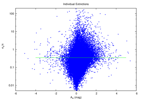
Figure 1: $A_{V}$ $vs.$ $\sigma_{\pi}/\pi$ diagram for the Hipparcos extinction sample with more than 85000 stars not commented as multiple or variable in $SIMBAD$. High proper motion stars are not included since a large fraction of them has a strange location in the $(B-V)_{obs}$ $vs.$ $V_{obs}+5(1+log\pi)$ diagram. Astrometry is from van Leeuwen (2007). The change in precision with $A_{V}$ taking place at $\sigma_{\pi}/\pi$ = 0.35 defines the sample used presently for the study of the local ISM

So far we have not considered the parallax precision. In Fig. 1 we have plotted $individual$ $A_{V}$ $vs.$ $\sigma_{\pi}/\pi$ where $A_{V}$ = 3.1$\times E_{B-V}$. Read from the bottom, where the attractive small errors presumably for nearby stars are located, we notice that the maximum positive extinctions increases with increasing $\sigma_{\pi}/\pi$ until a change takes place at $\approx$0.35. We take this dividing value as the upper limit for the relative precision. In fact no stars beyond $\sim$1 kpc has a better precision than this value. Most of the very negative extinctions belong to stars that has a tabular value $(B-V)_{obs}$ = 0.000 which obviously is not correct for the assigned spectral type. We have kept them in the sample though.

A diagram like $A_{V}$ $vs.$ $\pi$ will show the general run of extinction and should display the LB wall, if any. There is in fact such a wall-like feature present in Fig. 2 where a general rise in the extinction takes place at $\pi$$\approx$8 mas or 125 pc. A distance roughly corresponding to the maximum extent, apart from the tunnel directions, in Vergely et al. (2010).

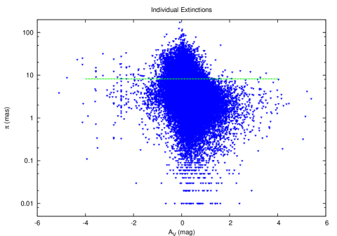
Figure 2: General variation of extinction with parallax for the Hipparcos extinction sample, the $\sigma_{\pi}/\pi$ = 0.35 confinement is not applied here. Notice the extinction discontinuity at $\pi\approx$ 8 mas (125 pc) roughly corresponding to the canonical ”radius” of LB

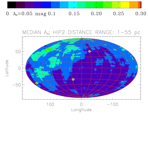
Figure 3: Sky distribution of median extinction for stars within 55 pc and with $\sigma_{\pi}/\pi<$0.35. The location of the far UV shadow clouds, lb165-32, lb27-31 and lb329+46 at 40, 45 and 65 pc are indicated by the diamonds, Berghoefer et al. (1998). A possible interpretation of this map could be: If the median $A_{V}>$ 0.1 mag the LB boundary is less than 55 pc away and if median $A_{V}<$ 0.1 mag the boundary is farther away. Grid for every 30 degrees in longitude and for every 15 degrees latitude

3 Sky Map for stars within 55 pc

On the average the Hipparcos extinction sample of $\sim$85.000 stars provide $\sim$two stars per square degree. Of course depending on the galactic latitude. The completeness is hard to assess in a statistical way since the Hipparcos input catalog was based on a variety of astrophysical proposals. Since the V magnitude for completeness is between 8 and 9 we do not measure large extinctions as is also evident from Fig. 2. But for our purpose, locating very nearby extinction, completeness for the extinction values is not necessary as long as a variation defining the LB boundary can be detected.

We cover the sky with a grid of overlapping pixels. Pixel size determined by requesting a number of stars per pixel permitting the computation of a median extinction for the distance range under study. In this note Fig. 3 presents the outcome for stars within 55 pc. The median $A_{V}$ values range from $\sim$0.05 mag to $\sim$0.3 mag and we note a marked difference between the north and south and between the 4 quadrants. This projection may be compared to Fig. 4 of Frisch, Redfield and Slavin (2011) showing $E_{B-V}$ contours for stars in the distance range from 50 to 100 pc. The distribution on Fig. 3 is almost identical but with smaller extinction values - which could be due to the different lenghts of the sight lines: $\leq$55 $vs.$ $\leq$100 pc.

In Fig. 3 we have also indicated the location of three diffuse clouds causing shadows in the far UV, Berghoefer et al. (1998). The clouds lb165-32, lb27-31, lb329+46 are removed $\leq$40, 45 and 65 pc respectively, just in the volume we are studying presently. As Fig. 3 shows the clouds are almost superposed on the boundary of the low density contour. Are they then part of the LB confinement? In fact they may not be because in Berghoefer et al. (1998) it was found that each of these small clouds was located in front of other clouds at 100, 135 and 125 pc respectively. These later distances agree much more to the canonical LB confinement. Recently Lallement, Vergely, Valette et al. (2013), from a very large photometric sample of $\approx$23.000 stars with various distance indicators, have presented a $E_{B-V}$ map for stars within 100 pc, among many others maps with different distance cuts, with a strong resemblence to Fig. 3. So, is the LB boundary, as indicated by the rise in color excesses/extinctions, real within 100 pc as indicated by the $E_{B-V}$ $\approx$ 0.1 mag contour, Frisch, Redfield and Slavin (2011), but not for stars within 55 pc with an $A_{V}$ $\approx$ 0.1 mag contour corresponding to $E_{B-V}$ $\approx$ 0.03 mag as the conclusion would be if the three shadow clouds mentioned really are $\approx$50 pc in front of the proper LB boundary?

But if we may rely on the median extinctions and the map in Fig. 3 and accept the median $A_{V}$ = 0.1 mag as defining the onset of extinction from the LB confinement we could possibly state that in the northern part of the first and second quadrant the LB limit is within 55 pc and in the southern part of the third and fourth quadrant it is further away.

4 Conclusions

We have constructed what was termed the Hipparcos extinction sample with about 85.000 distance extinction pairs. The classification originally in the Hipparcos Catalogue was supplemented with the $Michigan\ 5\ Catalogue$ classification of HD stars. We introduced a simple dwarf/giant separation of the $(B-V)_{obs}\ vs.\ V_{obs}+5(1+log\pi)$ in order to have a 2D classification of the stars with no luminosity class given in the Catalog.

Our main purpose has been to demonstrate that the Hipparcos extinction sample in addition to estimating distances to individual clouds, e.g. Knude and H$\o$g (1998), possibly also may be used to trace large scale features, extending over large fractions of the sky. It seems justified to conclude that further investigation of the Hipparcos extinction sample at larger distances may be worth while.

References

- Abt (2011) Abt, H.A., 2011, 141, 165
- Berghoefer et al. (1998) Berghoefer, T.W., Bowyer, S., Lieu, R., Knude, J. 1998, 500, 838
- de Geus, de Zeeuw and Lub (1989) de Geus, E.J., de Zeeuw, P.T., Lub, J. 1989, 216, 44
- Frisch, Redfield and Slavin (2011) Frisch, P.C. Redfield, S. and Slavin, D. 2011 49, 327
- Houk and Swift (1999) Houk, N. and Swift, C. 1999 , Department of Astronomy University of Michigan, Ann Arbor Michigan
- Knude (1987) Knude, J. 1987 171, 289
- Knude and Hg (1998) Knude, J. and Hg, E. 1998 338, 897
- Knude (2010) Knude, J. 2010 arXiv:1006.3676
- Lallement, Vergely, Valette et al. (2013) Lallement, R., Vergely,J.-L.,Valette, B., Pusspitarini, L., Eyer,L., Casagrande, L. 2013
- Perryman, Lindegren, Kowalevsky et al. (1997) Perryman, M.A.C., Lindegren, L., Kowalevsky, J. et al., 1997, 323, 49
- Reis et al’ (2011) Reis, W., Wagner, C., de Avillez, M.A., Santos, F.P. 2011 ApJ 734, 8
- Schmidt-Kaler (1982) Schmidt-Kaler, Th. 1982 Landolt-Boernstein VI 2b
- van Leeuwen (2007) van Leeuwen, F., 2007, 474, 653
- Vergely et al. (2010) Vergely, J.-L., Valette,, B., Lallement, R., Raimond, S. 2010, 518, A31