Gender homophily from spatial behavior in a primary school: a sociometric study

Abstract

We investigate gender homophily in the spatial proximity of children (6 to 12 years old) in a French primary school, using time-resolved data on face-to-face proximity recorded by means of wearable sensors. For strong ties, i.e., for pairs of children who interact more than a defined threshold, we find statistical evidence of gender preference that increases with grade. For weak ties, conversely, gender homophily is negatively correlated with grade for girls, and positively correlated with grade for boys. This different evolution with grade of weak and strong ties exposes a contrasted picture of gender homophily.

Highlights

• We investigate gender homophily in the spatial behavior of school children

• We use behavioral data on face-to-face proximity measured by means of wearable sensors.

• Strong ties provide evidence for gender homophily, which is slightly stronger for boys.

• For strong ties, gender homophily increases with age.

• For weak ties, gender homophily decreases with age for girls, while it increases for boys.

Introduction

The preference that individuals exhibit when they interact and build social ties with peers they consider to be alike is a well known feature of human behavior and is referred to as homophily (see McPherson et al. (2001) for a review). The traits that may influence human relationships are very diverse, ranging from physical attributes to tastes or political opinions. The question of which similarities mostly shape social networks is rather open, and the answer seems to depend on age and on the nature of the considered social ties. For example, gender or socio-ethnic homophily may vary over the lifespan of an individual, and sharing working habits is more important among coworkers than among friends. Together with other social mechanisms, such as triadic closure, prestige or social balance (Szell et al., 2010), homophily shapes social relationships and can play a role in the formation and stability of groups, possibly influencing the constitution of social capital (McDonald, 2011). Nevertheless, it is often difficult to assess quantitatively to which amount homophily contributes to social structures, because many of the traits that are considered important are changeable and might be modified by influence (Steglich et al., 2010). For example, similar smoking habits among teenagers may be important for the formation of new friendships, but at the same time an individual with many friends who smoke might be influenced to become a smoker. Unless panel data on social relationships and individual traits are available it is impossible to disentangle the above effects (Kossinets and Watts, 2009; Shalizi and Thomas, 2010), with the exception of traits, such as gender, racio-ethnicity or social background, that are almost immutable.

Investigating the correlation between gender and interaction patterns, therefore, allows to stay clear of the intricacies due to the interplay of homophily and social influence. A second advantage of studying homophily due to gender lies in its universality: gender is among the most important traits that shape interactions across cultures and, to different extents, it plays a role during the entire life span (Mehta and Strough, 2009; Maccoby, 2003). Finally, gender homophily in social networks has been shown to be linked to the broad issue of gender inequalities on the job market (McDonald, 2011). In the present analysis we will not make any distinction between sex and gender.

Here we study gender homophily among children as measured by monitoring their behavior in space. Our work is based on high-resolution networks of spatial proximity measured in a primary school in France over the course of two days. The data were collected using wearable devices that sense and log the face-to-face proximity relations of children over time. The use of such unobtrusive devices yields detailed information on the amount of time that children spend in close-range proximity, allowing us to build a behavioral network representation where nodes represent children and a link between two children indicates that those children have spent time in face-to-face proximity (i.e., they have engaged in a “contact”). Each link can be weighted by the amount of time the corresponding individuals have spent in contact. This network conveys information that is complementary to the social ties assessed by means of surveys or questionnaires. The time-varying proximity network captures objective information about one specific behavior in space, automatically and without incurring in the recall biases of subjective reports on spatial proximity to other individuals. Surveys and questionnaires, on the other hand, capture a much broader class of ties, and can integrate the full wealth of information on the subjective view of individual relationships. Here we aim at building a fine-grained picture of gender-related behavioral homophily in children, and leverage the detailed information on face-to-face proximity patterns provided by sensors to produce a quantitative assessment of gender-dependent and age-dependence proximity behavior. A natural question we want to address is the extent to which these behavioral findings are congruent with the picture available in the literature, based on declared friendship relations and on the observed actual behavior of children.

The article is structured as follows: a brief review of the literature on gender homophily and its evolution through the lifespan is presented first, together with some methodological perspectives on the use of electronic devices to measure behavioral aspects of human interactions. In the second part of the article we describe the dataset and the methodology used to collect it. Our results are presented in the third section. We report on statistical evidence of gender homophily in interaction patterns (i.e., proximity patterns in space), and we discuss the stability of neighborhoods from one day to the next. Finally, we use the high temporal resolution of the data to investigate how the correlation of homophily with age depends on the (behaviorally-defined) strength of the ties we consider. We obtain contrasted results that shed new light on the evolution of weak ties with age. We close with a short discussion and a call for further field research.

1 Background

Quantitative analyses on gender preferences date back to Moreno’s seminal work on sociometry (Moreno, 1953), in which he introduces network terminology to describe relations between children from kindergarten through eighth grade. His study relies on direct observations and interviews with children, and makes inferences about the variables that affect friendships. He shows that although young children up to the second grade prefer same gender mates, some of them also name friends of the opposite gender. This gender mixing then almost disappears, very few children making any mixed friendship up to the sixth grade.

Several studies have since confirmed and extended these results. A recent review (Mehta and Strough, 2009) shows in particular a consensus about the fact that gender homophily exists along the entire life span: it is already present in infants’ behaviors, increases up to a peak between 8 and 11 years (Maccoby, 2003), in agreement with Moreno’s study, and decreases afterwards, mainly because of the development of romantic relationships. It reaches a rather stable level among adults, although studies on this life period remain scarce.

More recently, some differences of interaction styles between boys and girls have been brought to light. The first and widely reported difference is that boys tend to have a broader social network than girls, who instead tend to make deeper and stronger relationships (Vigil, 2007; Lee et al., 2007). In particular, when children are asked to list their friends with no limitation on the number, boys name more friends than girls but most of the reciprocate nominations occur between girls. The evolution of interaction styles is moreover different for both genders. La Freniere et al. (1984) conclude from the direct observation of 193 children aged between 1 and 6 years that gender preferences increase earlier for girls than for boys, but later on they become stronger for boys than for girls. On the other hand, Martin and Fabes (2001) present a more moderate result. In a direct observation of 61 children between 39 and 74 months of age, they do not observe a significant correlation between age and the proportion of same sex playmates for the entire sample, but the correlation reaches a significant level when they consider boys only (this does not happen for girls). Indeed boys and girls behave differently, and differences in the amplitude of same gender preference have also been observed. Hayden-Thomson et al. (1987) asked 186 children about their positive, neutral or negative attitude toward all their classmates. While in the fourth grade girls are more positive towards boys than boys towards girls, the situation is reversed in the sixth grade. Shrum et al. (1988) reach similar conclusions from questionnaires identifying friendships.

During adolescence and the beginning of romantic relationships, girls show an earlier evolution in their attitude toward other sex mates than boys. Richards et al. (1998) report that girls declare to have frequent thoughts about the opposite sex one grade earlier than boys (but more moderately). They also declare to spend nearly twice as much time with boys as boys do with girls. This asymmetry may be explained by the fact that girls often have an older boy as second best friend outside school, while boys rarely report having girls as second best friends (Poulin and Pedersen, 2007).

Finally, stability of relationships, i.e. the maintenance of ties over time, is a facet of friendship that has recently drawn some interest (see Poulin and Chan (2010) for a review). It is known to increase during the primary school, which may be interpreted by the fact that concepts such as reciprocity, loyalty and ability of solving difficulties become more and more important in friendships at that age. Relationships between same sex peers are also more stable than mixed relationships but the empirical literature is still too shallow to conclude about gender differences in terms of stability.

While most analysis in this field rely on questionnaires, surveys or direct observations by adults, technological advances have led in the recent years to the emergence of new tools to investigate human behaviors and interaction patterns. In particular, wearable sensors can now be used to detect proximity (O’Neill et al., 2006; Hui et al., 2005; Pentland, 2007; Eagle et al., 2009; Salathe et al., 2010) and even face-to-face spatial relations (Cattuto et al., 2010; SocioPatterns, 2012).

The study of the networks resulting from this kind of ties implies a focus on behavioral networks defined in terms of spatial proximity, rather than on social networks as defined from friendship relations and built from questionnaires. These networks are known not to be completely disconnected: in particular, it has been shown that children interact four times more with members of their friendship group (identified with the social-cognitive map procedure) than with non-members (Gest et al., 2003). Moreover, as noted by Granovetter (1973), social ties are not adequately described as unidimensional relations, but are “(probably a linear) combination of the amount of time, the emotional intensity, the intimacy (mutual confiding), and the reciprocal services which characterize the tie”. The study of the relation between these different ingredients of a social tie is however far from trivial, especially as several of them are of qualitative nature.

In this respect, the use of wearable sensors embedded in unobtrusive wearable badges (Cattuto et al., 2010) allows to focus on the amount of time spent together by individuals, and to largely enhance our capabilities of quantitative studies of such behavioral aspects of the relationships networks. On the one hand, the method is unsupervised and does not require the continuous presence of observers, as in usual direct monitoring of behaviors. It has in fact already been used to monitor populations of several hundreds of individuals over several weeks (Isella et al., 2010), a task which would have been hardly possible with direct observation methods. On the other hand, it enables the precise, objective and reproducible definition of a tie in terms of location and body posture: a tie at time $t$ between a pair of individuals exists if they face each other in close proximity . Note that such behavioral ties are by construction reciprocal, while in the case of friendship networks it is quite common that a declared friendship is not reciprocated .

The use of sensors allows to address quantitatively research questions about homophily emerging from behavioral patterns, in a way that is complementary to studies based on friendship networks. We can investigate whether the friendship homophily is effectively translated into behavioral homophily as measured by the amounts of time children spend with same-gender and opposite-gender peers, and whether behavioral homophily exhibits the same features as friendship homophily. Some research questions can also be addressed in a more direct and objective way than through surveys or diaries: for instance, as the measurement can be carried out for several days, it is possible to measure directly the similarity of behaviors from one day to the next, and to compare the similarity of proximity patterns with same gender or opposite gender peers. The direct observation of close-range proximity of individuals allows us to assign a well-defined quantitative strength to each observed behavioral tie, for instance using the cumulated time that two individuals spend in face-to-face proximity. We can then define strong and weak ties on the basis of a chosen threshold for this quantitative strength. The ensuing classification of observed ties into “strong” and “weak” ones is of course purely behavioral and it depends on an arbitrarily chosen threshold. Regardless of the specific threshold value, such a classification achieves an unambiguous discrimination of behavioral ties into interactions that involve a strong commitment in terms of face-to-face presence and interactions that, conversely, correspond to a short engagement in close-range proximity. This makes it possible to contrast observations restricted to strong ties with observations restricted to weak ties, exposing the differential role of such behaviorally-defined tie strength. It also affords the investigation of specific properties of weak ties (as defined above), a notoriously difficult task when relying on surveys, diaries or even direct observation. Of course one can consider several other definitions of tie strength based on the time-resolved proximity data we use. For example, the number of interactions between individuals is another natural strength metric for ties, even though its relevance has been debated in the context of several research domains (Marsden and Campbell, 2012). The main argument is that contact frequencies are badly correlated with the other measures of tie strength, mostly because of contextual effects, which can be particularly relevant when considering interactions in a constrained environment (Cynthia M. Webster and Aufdemberg, 2001) . Here we focus on tie strength defined as the total (cumulated) time two individuals spend in close-range proximity because it is one of the simplest tie strength definitions we can define, it measures an intuitively important property of social behavior (i.e., the amount of time spent in physical proximity), and it hides the temporal complexity of multiple encounters, which is known to be bursty and far from trivial to model (González et al., 2008). Given this choice for the strength metric, we can study how the dependence of homophily with age differs between strong ties (long face-to-face engagement) and weak ties (short face-to-face engagement) ties, and how the time allocation to proximity in space differs across genders.

In the following, we investigate the above issues using high-resolution data on the face-to-face proximity patterns of children in a primary school, measured over two days, and originally collected in the context of an epidemiological study (Stehlé et al., 2011).

2 Data and methodology

Data on the face-to-face spatial proximity of more than $200$ school children was collected during two consecutive days in October 2009 in a primary school in Lyon, France (the school year starts in early September). This school is located in a wealthy district of a large city and belongs to the private catholic sector. Participants were asked to wear proximity-sensing electronic badges on their chest. The badges engage in bidirectional low-power radio communication, and can exchange radio packets only if the individuals who wear them are facing each other within a $1$m-$1.50$m range. Receiving stations (“readers”) located in the school classes and in the playground collect real-time information about the spatial proximity of participants. Cattuto et al. (2010) provide detailed information on the sensing infrastructure, and Stehlé et al. (2011) report a general analysis of the observed contact patterns. The wearable sensors are tuned so that the face-to-face proximity of two individuals wearing them can be assessed over an interval of $20$ seconds with a probability in excess of $99$%. Two individuals are said to be in contact if their badges exchange radio packets during a $20$-second time window, and the contact is considered interrupted if the badges cannot exchange packets over a $20$-second interval. Thus the minimum duration of a contact is $20$ seconds and all measured contact durations are multiples of $20$ seconds. We emphasize once again that the sensors measure the face-to-face proximity of individuals, and not the possible occurrence of conversations or physical contacts.

The primary school under study is composed of $10$ classes, divided in $5$ grades, labeled 1A, 1B, …, 5A, 5B (two classes for each grade). The age of children ranges between 6 and 12 years. The data were collected over two school days, from 8:30am to 5:15pm. Only interactions taking place on the school grounds were recorded. It is worth noting that slightly more than one child in three leaves the school premises for lunch, which leads to a relative drop of activity during the lunch break. All of the $10$ teachers and $96$% of the children ($232$ out of $241$) took part in the data collection. The $9$ remaining children were either missing on both days or received a badge that was defective and had to be removed from the dataset.

Class	Girls	Boys	Total	Class size
1A	11	10	21	24
1B	13	12	25	25
2A	14	9	23	25
2B	15	11	26	26
3A	9	14	23	24
3B	11	11	22	22
4A	8	11	19	23
4B	10	13	23	24
5A	10	11	21	24
5B	11	13	24	24

Table 1: Number of girls and boys in each class for which contact data and gender have been collected.

Each individual is uniquely associated with one wearable badge and, through that, to a unique numeric identifier. The identifier is only associated with anonymous metadata for each individual: school class, gender, year and month of birth. All the statistical treatment of the data is performed in an anonymous way. The metadata was collected for $227$ out of $232$ participating students. The difference is accounted for by participants whose badge was accidentally replaced during the deployment, breaking the connection between the badge identifier and the participant metadata. We restrict our sample to this subpopulation of $227$ children ($94$% of the children in the school), composed of $112$ girls and $115$ boys, and we do not consider the data relative to teachers. We can reasonably assume the absence of any selection bias, as the exclusion from the studied population is not related to gender or behavior. Table 1 gives the corresponding numbers of boys and girls in each class.

The proximity-sensing infrastructure records the time and duration of each face-to-face proximity event (or “contact”, in the following), thus it is possible to construct an aggregated network of face-to-face proximity over a given period of time – for instance one day – where nodes represent individuals, and edges link individuals who have been in contact at least once during the day. Each edge corresponds therefore to a sequence of contact events between the two linked individuals.

We do not have information on whether children conform to pre-defined seating arrangements during class time, nor whether teachers control or influence the seating patterns within classes. In order to remove possible biases due to such factors, we study the spatial proximity of children when they have maximum freedom of associating with one another: we restrict our analysis to contacts recorded in the playground and canteen of the school, which overall account for $32\,027$ contact events ($41\%$ of the recorded contacts). The recorded contacts are used to construct an aggregated weighted network, in which nodes represent children and pairs of nodes are connected by an edge if the corresponding pair of children has met at least once during the two days. The weight $w_{ij}$ of an edge between child $i$ and child $j$ is here defined as the cumulated duration of all their contacts. The resulting network comprises $227$ nodes and $7070$ weighted edges.

3 Results

Though we only consider contacts occurring in the playground or in the canteen, the contact patterns are highly determined by the grade and class structure of the school. Figure 1 shows the degree of contact between classes: each matrix element (row X, column Y) is greyscale-coded according to the sum of contact durations between all pairs of children belonging respectively to classes X and Y, i.e., $W_{XY}=\sum_{i\in X}\sum_{j\in Y}w_{ij}$ (the weight $W_{XX}$ for contacts inside the same class X is twice the sum of all contact durations among the children of class X). The high values along the diagonal of the matrix indicate that most contacts occur between pairs of children belonging to the same class. The division into grades is responsible for the visible block-diagonal structure ($2\times 2$ darker squares along the diagonal). Lower grades (1st to 3rd) also have less contact with higher grades (4th and 5th), with the exception of one class in the 1st grade. Most of this structure can be understood in terms of the schedule of class breaks and turns at the canteen. In particular, in France, the first three grades (called “cours préparatoire” and “cours élémentaire”) are rather clearly separated from the fourth and fifth grades (called “cours moyen”).

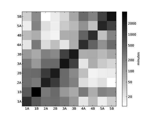
Figure 1: Class-wise contact matrix: the matrix entry for row X and column Y indicates the total duration of all contacts recorded in the playground and in the canteen between class X and class Y, over the course of two days. The matrix values, expressed in minutes, are logarithmically greyscale-coded as shown in the legend.

Figure 2 shows the cumulative weight histograms for boy–boy, boy–girl or girl–girl edges in the aggregated contact network, and provides a first indication of gender-related differences. Edges between boys are more frequent than between girls ($1724$ vs $1261$) whilst there are almost as many girls as boys ($N_{g}=112$ girls vs $N_{b}=115$ boys). There are more than twice as many mixed edges than edges between girls ($2553$ vs $1261$), but far less than twice the number of edges between boys. The three cumulative histograms shown in Fig. 2 indicate that mixed-gender edges tend to correspond to shorter cumulated interactions relative to edges linking same-gender individuals: the mean weights of mixed-gender and same-gender edges are $118$ s and $242$ s, respectively. Moreover, edges between girls have on average higher weights than edges between boys, with mean weights of $265$ s and $225$ s, respectively.

In this behavioral aggregated network the average degree is equal to $62.3$, and has a higher value for boys than for girls ($67.1$ and $57.3$, respectively). This difference is significant at the $10\%$ threshold (tested with a one-sided Wilcoxon test, $p=0.06$). When considering the subgraph defined by edges with weight of at least $5$ min, the average degree is $8.0$, with a significantly higher value for boys than for girls ($9.0$ vs $7.0$, $p=0.07$).

These two observations, that relate to the behavior of children, are in agreement with results on friendship network structures, and in particular with the literature about differences on group size and level of intimacy, as reviewed by Vigil (2007). They support the hypothesis that men and women (here, boys and girls) arbitrate differently between maintaining a large social group and having more intimate and secure relationships.

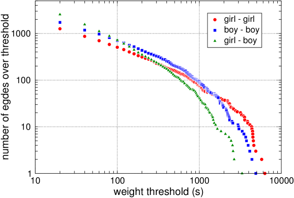
Figure 2: Cumulative histograms of edge weights of the contact network aggregated over two days. Edges are divided into three categories according to the gender of the connected nodes (boy–boy, boy–girl or girl–girl).

Figure 2 also clearly shows that cumulated contact durations are smoothly and broadly distributed, extending over a large range of times. The behavioral data on face-to-face proximity lack any intrinsically characteristic time scale, i.e., no typical duration can be defined for any type of contact.

3.1 Statistical evidence of gender homophily

In this section, we aim at testing statistically the evidence of gender homophily. Our approach consists in comparing the aggregated contact network with null models of graphs in which the probability that an edge connects two nodes is independent of node genders, to assess the probability that the observed contact network arises from such an arrangement of contacts between individuals.

We first restrict the study to contacts occurring within each class: the school schedule constrains contacts between classes, hence we cannot assume that children have the same opportunity to make strong ties within and across classes. Moreover, we only consider edges with weight of at least $5$ minutes, i.e., whose contacts have a cumulated duration of at least $5$ minutes over the two days of data. The aggregated contact network has $531$ such edges, and in the following we will indicate them as strong ties, in reference to Granovetter’s terminology. The threshold of $5$ minutes is arbitrary: it has been chosen to be large enough to eliminate weak ties that will be shown later (Sec. 3.4) to have different properties with respect to gender homophily, and small enough to retain a sufficient number of edges for statistical analysis. We have checked that all of our results are robust with respect to changes in the $5$ minutes threshold. We also note that the cumulated contact durations, the total number of contact events, and the longest observed contact durations, are strongly correlated, so that longer cumulated durations correspond to longer single contact events and that a filtering procedure on the cumulated duration or on the maximal duration of a contact would lead to the same results.

In order to test for homophily in a given class with $N_{b}$ boys and $N_{g}$ girls we consider the numbers of strong ties of each type: the total number $E$ of strong ties in the class is divided into $E_{gg}$ ties linking two girls, $E_{bb}$ ties linking two boys, and $E_{bg}$ ties involving a boy and a girl ($E=E_{gg}+E_{bb}+E_{bg}$). Testing for homophilous behavior amounts to comparing the empirical values of these parameters against the values they assume for null models in which the existence of a tie is not correlated with the gender of the individuals it links.

It is possible to design several null models of different complexity that control for different features of the empirical data. We begin by defining a null model that controls for the overall density of the contact network as well as for the difference in average degrees of boys and girls that was reported above. We want the null model to have the same numbers $N_{b}$ and $N_{g}$ of boys and girls and the same number of edges $E$, i.e., the same density as the empirical contact network. Moreover, let us denote the average degree of boys and girls respectively by $k_{b}=(2E_{bb}+E_{bg})/N_{b}$ and $k_{g}=(2E_{gg}+E_{bg})/N_{g}$. Since $N_{b}k_{b}+N_{g}k_{g}=2E_{bb}+2E_{bg}+2E_{gg}=2E$, a constraint on $k_{b}$ also determines $k_{g}$ (and vice versa). We can therefore control for the different values of $k_{b}$ and $k_{g}$ by fixing, equivalently, $k_{b}$, $k_{g}$ or $k_{b}-k_{g}$. Here we choose the first solution. Fixing $E$ and $k_{b}$ places two constraints on the three variables $E_{gg}$, $E_{bb}$ and $E_{bg}$, leaving the null model with a one dimensional random variable left, whose value will account for the degree of homophily in the allocation of the $E$ ties.

As it turns out, not only we can set $k_{b}$ (and hence $k_{g}$) to match the empirical values: we can actually design a null model that preserves the degree of each node, and thus, in particular, the average degrees $k_{b}$ and $k_{g}$. To this aim, we construct an ensemble of random graphs with $N_{b}$ boys and $N_{g}$ girls having the same degrees as in the empirical data by applying to the empirical network the reshuffling procedure by Maslov et al. (2004), which preserves the degree of each node and hence the average degree for every group of nodes.

In summary, our first null model corresponds to random graphs with $N_{b}$ boys, $N_{g}$ girls, a fixed number of ties $E$, and a fixed degree sequence (and as a consequence fixed average degrees $k_{b}$ and $k_{g}$ for the boys and the girls). We can therefore test for homophilous behavior in the class by computing the distribution of the fraction $E_{bg}/E$ of ties linking nodes of opposite gender in the null model, and comparing it to the empirical value of this ratio. To this aim we consider the following null hypothesis:

$H0$: the observed fraction $E_{bg}/E$ of ties involving a boy and a girl is compatible with that of a random graph in which nodes are labeled by gender ($N_{b}$ boys and $N_{g}$ girls), the degree sequences is that of the empirical network, and the existence of a tie between two nodes does not depend on their gender.

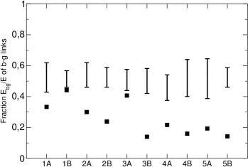
Figure 3: Statistical test of gender homophily for contacts within each class, restricted to contacts of cumulated duration of at least $5$ minutes over two days. Error bars indicate the $95\%$ confidence interval of acceptance of the null hypotheses of gender indifference. Symbols indicate the empirical fraction of ties involving a boy and a girl. Left: the error bars correspond, for each class, to the $95\%$ confidence interval for the values of $E_{bg}/E$ obtained under the null hypothesis $H0$. Right: same for the null hypothesis $H0^{\prime}$.

The left-hand panel of Fig. 3 shows for each class the region of acceptance of the null hypothesis $H0$ at the $5\%$ threshold. The empirical values are compatible with $H0$ in none of the classes, with values of the fraction of ties joining students of different gender below the $95\%$ confidence intervals. Hence we can reject the null hypothesis $H0$ of gender independence of the edges.

It is however important to remark a limitation of the null model considered above. The null hypothesis $H0$ disregards all knowledge about the specific structure of the network (the correlations between the numbers of neighbors of individuals in contact, the size of friendship clusters, etc.), except for the set of degrees of boys and girls. In particular, a strong tie may exist between two children independently of the fact that they may share many contacts. It is on the contrary known that many triangles exist in the aggregated contact network, just like in many social networks.

To overcome this limitation, we design a different null hypothesis: we consider the network of strong ties as fixed, and we randomly assign the gender of each node, preserving the numbers of girls and boys in each class. Under such a null hypothesis genders are interchangeable and the network formed by the strong ties is independent from the gender attributes. As previously discussed, we need to control for the difference in the average degrees of boys and girls. To this aim, we fix the network structure and we consider all possible allocations of genders to nodes in which not only the number of girls and boys are equal to their empirical values, but also the average degree of boys (or equivalently of girls) is exactly equal to its empirical value $k_{b}$. The corresponding null hypothesis can now be written as

$H0^{\prime}$: the observed fraction $E_{bg}/E$ of ties involving a boy and a girl is compatible with that of a graph having exactly the same topological structure as empirically observed, with $N_{b}$ nodes labeled as boys and $N_{g}$ as girls in a random fashion, in such a way that the average degree of boys is fixed to its empirical value (and hence the average degree of girls is also fixed to its empirical value).

As shown in Fig. 3, the results are very similar to the previous case and still provide statistical evidence for same-gender peer preference in all classes.

3.2 Gender homophily from individual-based indices

While the analysis of the previous paragraph was based on a global measure (the number of same-gender ties inside a group), heterogeneity between individuals can also be investigated through an individual index.

3.2.1 Within class ties

Let us first consider the same network as in the previous paragraphs, i.e., restricted to strong ties (cumulated durations of contacts of at least $5$ minutes) between children within each class.

For each node $i$ with at least one neighbor in this strong-tie network ($215$ children out of the previous $227$), we compute the proportion of same gender peers among its $k_{i}$ neighbors. We call this index the individual homophily index, and we denote it by $P_{k}^{sg}(i)$. This index is equal to $1$ if the considered child has only same-sex neighbors and equal to $0$ if all the neighbors are of the opposite sex. To interpret this index as a preference towards same-gender peers, the values of $P_{k}^{sg}(i)$ have to be compared with some baseline homophily. In the case of within class ties, this baseline homophily can be quantified with the ratios $(n_{b}-1)/(n_{g}+n_{b}-1)$ for boys and $(n_{g}-1)/(n_{g}+n_{b}-1)$ for girls (the $-1$ is there because an individual cannot have a link with him/herself), where $n_{b}$ and $n_{g}$ stand respectively for the number of boys and girls in the studied class. These values take the gender ratio inside each class into account. Given any null model for which children would be indifferent to gender, the mean value of the individual homophily index would be given by these baselines. Figure 4 gives for each class the boxplot of the individual homophily index, computed separately for boys and for girls, together with the baseline homophily values. We observe that most of the time, the baseline value is not contained between the first and the third quartiles of the empirical distribution of the index, thus illustrating the evidence of a gender homophily within classes as quantified by the distribution of the individual homophily indices, even for small grades.

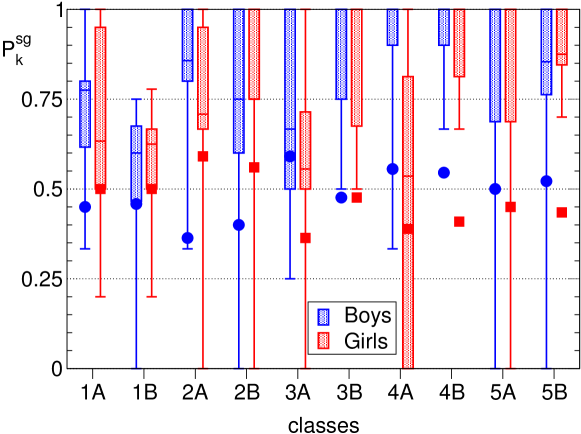
Figure 4: Boxplots of the same gender preference index $P_{k}^{sg}$, computed in each class separately for boys (blue) and girls (red). The center of the box indicates the median, its extremities the lower and upper quartiles, and whiskers indicate the smallest and largest values. The symbols indicate the baseline homophily for each gender in each class.

3.2.2 Inter- and intra-class ties

We have considered so far ties within classes, corresponding to interactions recorded in the playground or in the canteen. The class structure makes it indeed easier to study individual preferences of children to interact with same-sex peers: given that the children of a given class share the same schedule, we can assume that each child has an equal opportunity to interact for long (more than $5$ minutes) with same-class mates. This has allowed us to construct null models and baseline homophily values to be compared with the empirical data.

However, the equal opportunity assumption has to be considered with discernment. The setting allows to record only interactions within the school premises. It is very likely that some of these children see each other during activities outside the school or in the neighbourhood of their living places. In that case, the opportunities with these children would not be the same as with the others. If the opportunities are correlated with gender (typically in the case of sport activities), then the observed same-gender preference would partly result of gender-correlated opportunities. The main difficulty here comes from the fact that we do not ask children to report on their preference but we deal with behavioral information on how they interact with each other. We now change our perspective in considering only the proportion of same-gender mates these children interact with during breaks and lunch, in a purely descriptive way, relaxing the condition of being part of the same class. We consider the network composed of strong ties (cumulated durations of contacts of at least $5$ minutes, as above) linking children belonging to either the same class or different classes, for a total of $795$ ties .

In this case, since the number of boys and girls in the school are almost the same, the same gender preference index should be compared to a gender-balanced neighborhood for which the index would take the value $\approx 0.5$ ($112$ girls vs $115$ boys). Figure 5 reports the corresponding boxplots for each class, separately for boys and for girls. The dispersion of the index distribution is large, as indicated by the size of the box and the whiskers. While it happens that a child has no ties with other children of the same gender, most values of the index are rather high: same-gender homophily is present in all grades, for both genders. Moreover, the figure seems to indicate that boys tend to have a higher individual homophily index than girls, and that this index increases with grades (we will examine this point in Sec. 3.4).

Figure 5: Same as Fig. 4 for the network of strong ties at the whole school level: Boxplots of the same gender preference index $P_{k}^{sg}$, computed separately for boys (blue) and girls (red). The center of the box indicates the median, its extremities the lower and upper quartiles, and whiskers indicate the smallest and largest values.

The statistical difference between boys and girls can be estimated through a one-sided Wilcoxon test. This non-parametric test is preferred to a parametric one (such as ANOVA) because it does not require any assumption on the form of the distribution of the underlying random variable that generates the heterogeneity of individual homophily index. We test the null hypothesis that the averages of the individual homophily index are the same for boys and girls, against the one-sided alternative hypothesis that the average is higher for boys than for girls. For the 4th and the 5th grades the null hypothesis is rejected at the $10\%$ threshold, meaning that individual homophily is higher for boys and for girls only for the two highest grades, but that, even in these cases, the effect is only marginally significant.

Interestingly, and despite the largest parts of the distributions shown in Fig. 5 are above 1/2, some children have most of their strong ties with children of the opposite sex. The interpretation proposed by Snijders  is that this situation could be socially allowed under the condition that the neighbors have as well many contacts with individuals of the other sex. To check this hypothesis, we define a two-step homophily index for each node $i$, slightly modifying the definition of the alters’ covariate-average defined by Ripley et al. (2011):

$$P_{k2}^{sg}(i)=\frac{1}{k_{i}}\sum_{j\in\mathcal{V}(i)}\frac{k_{j}(\mbox{gender}_{i})}{k_{j}}\ .$$

In this expression, $\mathcal{V}(i)$ denotes the set of the $k_{i}$ neighbors of node $i$, $k_{j}$ is the number of neighbors of $j$, and $k_{j}(\mbox{gender}_{i})$ is the number of neighbors of $j$ having the same gender as $i$. $P_{k2}^{sg}(i)$ is therefore the average over the nodes $j$ belonging to the neighborhood $\mathcal{V}(i)$ of node $i$, of the proportion of $j$’s neighbors who have the same gender as node $i$. Figure 6 provides the scatter plot of this two-step homophily index with respect to the previous individual homophily index $P_{k}^{sg}(i)$. Boys have on average a higher two-step homophily index than girls (p-value $<5\cdot 10^{-3}$ with a one-sided Wilcoxon test). Moreover, if we consider egos having a majority of neighbors of the opposite sex ($P_{k}^{sg}<0.5$), the neighbors themselves have on average more ties with children of the same sex as ego than ego her/himself ($P_{k2}^{sg}(i)>P_{k}^{sg}$).

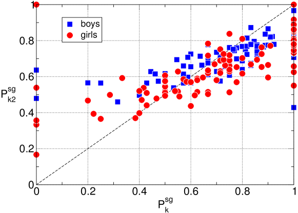
Figure 6: Scatter plot of the two-step homophily index $P_{k2}^{sg}$ vs the individual homophily index $P_{k}^{sg}$, computed separately for boys (blue) and girls (red). The first bisector is represented by a dashed line.

3.3 Similarity of neighborhoods in different days

We have focused in the previous paragraphs on an aggregated and filtered view of the behavioral network of proximity between children. In this view, we have considered the durations of contacts aggregated over the whole measurement and used this information to define and focus on the strong ties. As the data is time-resolved, it is however possible to compare the behavior of children in different days, in a way that takes into account the contact durations in a more complete way, and in order to understand the interplay between gender homophily and the daily repetition of contact patterns. We emphasize that we are here considering the similarity between the behavioral networks of children in successive days, rather than the evolution (and possible decay) of social links in social networks, that take place on longer timescales (Burt, 2000, 2002).

To this aim, we quantify the similarity between the neighborhood of each individual $i$ in day $1$ and day $2$ through the cosine similarity

$$\sigma(i)=\frac{\sum_{j}w_{ij,1}w_{ij,2}}{\sqrt{(\sum_{j}w_{ij,1}^{2})(\sum_{j}w_{ij,2}^{2})}}\,,$$ (1)

where the weight $w_{ij,1}$ is the cumulated time spent in face-to-face interaction between $i$ and $j$ during day $1$, and $w_{ij,2}$ is the corresponding time during day $2$ (children absent in one of the two days are naturally excluded from this analysis).

We also consider two different similarity definitions that separately measure the similarities of the same-gender and of the opposite-gender neighborhoods across days ($\sigma_{sg}(i)$ and $\sigma_{og}(i)$, respectively), by restricting the sums in Eq. 1 to neighbors $j$ who have the same (or the opposite) gender as $i$:

$$\sigma_{sg}(i)=\frac{\sum_{j\in{\cal V}_{sg}(i)}w_{ij,1}w_{ij,2}}{\sqrt{(\sum_{j\in{\cal V}_{sg}(i)}w_{ij,1}^{2})(\sum_{j\in{\cal V}_{sg}(i)}w_{ij,2}^{2})}}\,,$$ (2)

where the sums over $j$ are restricted to the same-gender neighborhood ${\cal V}_{sg}(i)$ of $i$, and

$$\sigma_{og}(i)=\frac{\sum_{j\in{\cal V}_{og}(i)}w_{ij,1}w_{ij,2}}{\sqrt{(\sum_{j\in{\cal V}_{og}(i)}w_{ij,1}^{2})(\sum_{j\in{\cal V}_{og}(i)}w_{ij,2}^{2})}}\,,$$ (3)

where the sums over $j$ are restricted to the opposite-sex neighborhood ${\cal V}_{og}(i)$ of $i$.

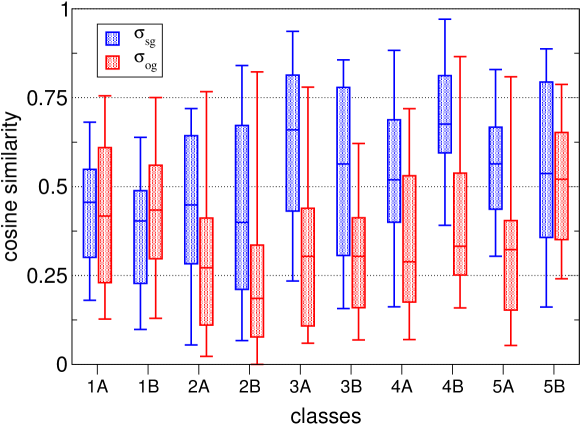
Figure 7: Distributions of cosine similarities between the neighborhoods of the individuals of each class in days 1 and 2, restricted to same gender neighborhood $\sigma_{sg}$ and to opposite gender neighborhood $\sigma_{og}$.

Figure 7 displays the boxplots of the distributions of $\sigma_{sg}$ and $\sigma_{og}$ for each class. We test the null hypothesis that the averages of $\sigma_{sg}$ and $\sigma_{og}$ are the same against the one-sided alternative hypothesis that the average is higher for $\sigma_{sg}$ than for $\sigma_{og}$. Through a Wilcoxon test, the null hypothesis is rejected at the $5\%$ threshold for $6$ classes (one in the 2nd grade, one in the 5th grade, and all classes of the 3rd and 4th grades), and with a p-value of $0.125$ for the other class of the 2nd grade. This shows that the same-gender part of the neighborhood of an individual is statistically more stable from day 1 to day 2 than the opposite-gender part of the neighborhood, in agreement with the literature reviewed by Poulin and Chan (2010). On the other hand, the stability of a child’s neighborhood is not significantly dependent on her/his gender: a Wilcoxon test of the null hypothesis that the averages of $\sigma$ are different for boys and girls leads to p-values larger than $0.3$ except for one class of the third grade with $p=0.06$.

3.4 Evolution of individual homophily with age

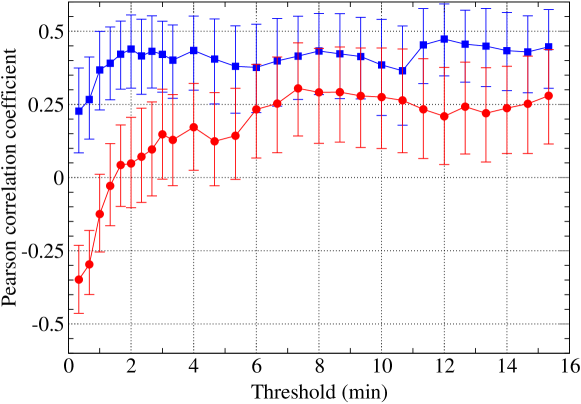
Figure 8: Pearson correlation coefficients between age and same-gender homophily index $P_{k}^{sg}$, as a function of the threshold on edge weights. The correlation is computed separately for boys (blue squares) and for girls (red circles). Error bars indicate the bootstrap $90\%$ confidence interval, computed with $2000$ resamples.

In subsection 3.2.2, we noted in Fig. 5 a positive correlation between the same-preference index and grade. This would mean that older children tend to have more contacts with same-gender mates. This behavioral trend is in agreement with previous studies focusing on social relations (Mehta and Strough, 2009; Maccoby, 2003; Moreno, 1953). The information we have about the age of children allows us to explore this issue in more detail, taking advantage of the quantitative temporal information encoded into the behavioral network. We thus investigate quantitatively the correlation between age and individual homophily index, separately for boys and girls, and as a function of the weights of the links considered. Figure 8 shows the Pearson correlation coefficient between age and same-gender preference index, as a function of the threshold on the cumulated contact duration ($5$ minutes in the analysis above): when this threshold is equal to $20$ seconds (the minimum duration of a contact) we retain all ties, while on increasing it less and less edges are kept (the strongest ones).

For both boys and girls, when we consider edges that correspond to a cumulated interaction time of at least $100$ seconds (over $2$ days), the correlation between the individual homophily index and age is positive, and it is higher for boys than for girls. However, when weaker ties are retained (i.e., edges corresponding to shorter cumulated times), the correlation is instead negative for girls. This means that the evolution of homophilous behavior with age is different for weak and strong ties, and between boys and girls. A closer inspection reveals that for interactions of cumulated duration shorter than $3$ minutes the number of same-gender mates decreases with age for both genders, and that the number of opposite-gender neighbors decreases even faster for boys, while it increases for girls. For contacts of cumulated duration larger than $5$ minutes, on the other hand, the number of same-gender mates decreases for boys and stays almost constant for girls, while the number of opposite-gender neighbors decreases for both genders. The increase in the number of short encounters that girls have with boys may be related to their earlier evolution in their attitude towards the other sex, as pointed out by Richards et al. (1998) and Poulin and Pedersen (2007). The same overall picture emerges when analyzing the correlation of the same-gender preference index with school grade rather than age, with a slightly weaker correlation of individual homophily index and grade for boys.

As an aside, it may be noted that for high enough values of the threshold some children become isolated in the network, meaning that they have no interactions with other children that account for a longer time than the threshold. This isolation does not affect equally children who have either skipped or repeated a grade ($N=23$), and are thus younger (or older) than other children of the same class, and the other children ($N=204$). At the $5$ minute threshold, $5$ children out of the $23$ become isolated, compared to $7$ for those who have the same age as their classmates. The relative risk for the children who have either repeated or skipped a grade to become socially isolated, compared to the other children, is equal to $6.33$ (a corresponding odds ratio of $7.8$), indicating that children who skip or repeat grades might be more exposed to social exclusion. However, the data collect took place relatively early in the year (Fall), at a time were some children are still new to others. It is thus plausible that the social exclusion would be weaker later in the school year.

4 Discussion

The use of wearable sensors represents a new tool in the study and description of child behavior. With respect to direct observation or contact diaries, the presented methodology, based on unobstrusive devices that can be worn during several consecutive days, has some advantages. As it is unsupervised, it is much less limited in terms of population size or duration of study and does not suffer from recall biases. It also allows us to build a precise definition of a behavioral tie, and gives access to quantitative information on the duration of face-to-face proximity events between children. It yields daily complete networks of face-to-face interactions of the school population, with ties weighted according to behavioral information (who spends time with whom), independently from recall biases.

It allows one therefore to investigate in some detail to which extent features of friendship social networks, described in previous literature mainly based on name-generator questionnaires, are effectively recovered in terms of quantitative behavioral patterns. Several features are indeed observed with statistical significance: 1) gender homophily is present in all grades of the primary school; 2) gender homophily reaches a higher level for boys than for girls in the 4th and 5th grades; and 3) gender homophily tends to increase with age for strong ties, at a higher rate for boys than for girls.

The quantification of face-to-face proximity behavior allowed us to elucidate subtle aspects of behaviorally-defined gender homophily, including gender-based and age-dependent properties. In particular, we have shown that same-gender ties are more similar across different days than mixed-gender ties, which are subject to higher inter-day variability. The unbiased discrimination of behaviorally-defined strong and weak ties is a specific advantage of the behavioral proxy we selected: information on weak ties in our framework is as accessible and reliable as information about strong ties, in contrast to data obtained from surveys or diaries, for which different kinds of cognitive and recall biases may apply depending on tie strength. The definition of tie strength in terms of cumulated face-to-face time, together with the objective empirical access to the time individuals spend in face-to-face proximity, allowed us to probe how gender-based homophily in the proximity behavior depends on tie strength. This showed that, for strong ties, individual homophily tends to increase with age at a higher rate for boys than for girls. Conversely, for weak ties, the individual homophily is positively correlated with grade for boys, while, remarkably, it is negatively correlated with grade for girls.

The empirical study of human interactions, and in particular the influence of peer behaviors on individual outcomes is of major interest in a broad range of social sciences, such as human behavior, sociology, economy or education economy, and organizational science (Manski, 1993). The collection of empirical social network data represents however a major barrier for the understanding of social influences, especially in the context of models such as those introduced by Doreian (1980) or more recently by Steglich et al. (2010). In this context, the development of unsupervised methodologies that allow researchers to collect large-scale, high-resolution dynamical data on human behavior in a reproducible manner is a valuable asset that deserves some comments.

As previously mentioned, new technologies entail important advantages in terms of ease of deployment and measures at large scale and for consecutive days. Re-test studies and comparisons can be easily carried out in order to validate trends or to determine which features are context-specific. It has of course to be underlined once again that unsupervised detection of proximity patterns gives access to a behavioral proxy rather than on real information about social interactions (e.g., the different types of relationships are disregarded). This behavioral proxy can be thought of as one of the multiple components of a social relation, that can be here quantitatively measured in a way that avoids informant biases such as the limited recall of individuals about their contacts and acquaintances. It represents an important tool to assess the similarity between behavioral and friendship homophily, and, given this similarity, represents a very interesting tool for further studies of behavioral and social networks, in particular for the study of the structure and evolution of weak ties.

The present study naturally stimulates further research avenues. First, it would be interesting to investigate the (quantitative) robustness of the results when different schools and different moments of the school year are considered, and when a given population is followed for longer periods. To this aim, deployments of the infrastructure are planned for whole weeks, in different schools, and in different periods of the year. The evolution of both age and gender behavioral homophily along the school year could thus be assessed. Moreover, more elaborate RFID badges endowed with an accelerometer (under development) could allow us to test a possible correlation between gender homophily and different amounts of activity of boys and girls. Finally, studies that would allow to make more accurate comparisons between various ways of capturing social and behavioral interactions would be of great interest. To this aim, detailed comparison methods between automated and supervised data collection methods, such as surveys, should be developed and are crucially important to assess the specific limitations and potentials of the methodology.

References

- Burt (2000) Burt, R. S., 2000. Decay functions. Social Networks 22 (1), 1 – 28.
- Burt (2002) Burt, R. S., 2002. Bridge decay. Social Networks 24 (4), 333 – 363.
-
Cattuto et al. (2010)
Cattuto, C., Van den Broeck, W., Barrat, A., Colizza, V., Pinton, J.-F.,
Vespignani, A., Jul. 2010. Dynamics of person-to-person interactions from
distributed rfid sensor networks. PLoS ONE 5 (7), e11596.
URL http://dx.doi.org/10.1371/journal.pone.0011596 - Cynthia M. Webster and Aufdemberg (2001) Cynthia M. Webster, L. C. F., Aufdemberg, C. G., 2001. The impact of social context on interaction patterns. Journal of Social Structure.
- Doreian (1980) Doreian, P., 1980. Linear models with spatially distributed data. Sociological Methods & Research 9 (1), 29–60.
- Eagle et al. (2009) Eagle, N., Pentland, A., Lazer, D., 2009. Inferring social network structure using mobile phone data. Proceedings of National Academy of Sciences 106 (36), 15274–15278.
- Gest et al. (2003) Gest, S. D., Farmer, T. W., Cairns, B. D., Xie, H., 2003. Identifying children’s peer social networks in school classrooms: Links between peer reports and observed interactions. Social Development 12 (4), 513–529.
-
González et al. (2008)
González, M. C., Hidalgo, C. A., Barabasi, A. L., 2008. Understanding
individual human mobility patterns. Nature 453, 479.
URL doi:10.1038/nature06958 - Granovetter (1973) Granovetter, M., 1973. The strength of weak ties. American Journal of Sociology 78, 1360 – 1380.
- Hayden-Thomson et al. (1987) Hayden-Thomson, L., Rubin, K. H., Hymel, S., 1987. Sex preferences in sociometric choices. Developmental Psychology 23 (4), 558 –562.
- Hui et al. (2005) Hui, P., Chaintreau, A., Scott, J., Gass, R., Crowcroft, J., Diot, C., 2005. Pocket switched networks and human mobility in conference environments. In: WDTN ’05: Proceedings of the 2005 ACM SIGCOMM workshop on Delay-tolerant networking. ACM, New York, NY, USA, pp. 244–251.
- Isella et al. (2010) Isella, L., Stehlé, J., Barrat, A., Cattuto, C., Pinton, J.-F., Broeck, W. V. D., 2010. Whatʼs in a crowd? analysis of face-to-face behavioral networks. Journal of Theoretical Biology 271, 166–180.
- Knoke and Yang (2008) Knoke, D., Yang, S., 2008. Social network analysis, 2nd Edition. No. 07-154 in Quantitative applications in the social sciences. Sage Publications.
- Kossinets and Watts (2009) Kossinets, G., Watts, D. J., 2009. Origins of homophily in an evolving social network. American Journal of Sociology 115, 405–450.
- La Freniere et al. (1984) La Freniere, P., Strayer, F. F., Gauthier, R., 1984. The emergence of same-sex affiliative preference among preschool peers: a developmental/ethological perspective. Child development 55 (5), 1958–1965.
- Lee et al. (2007) Lee, L., Howes, C., Chamberlain, B., July 2007. Ethnic heterogeneity of social networks and cross-ethnic friendships of elementary school boys and girls. Merril-Palmer Quaterly 53 (3), 325 – 346.
- Maccoby (2003) Maccoby, E. E., 2003. The Two Sexes: Growing Up Apart, Coming Together, 5th Edition. Belknap Press of Harvard University Press.
- Manski (1993) Manski, C. F., 1993. Identification of endogenous social effects: The reflection problem. The Review of Economic Studies 60 (3), 531–542.
-
Marsden and Campbell (2012)
Marsden, P. V., Campbell, K. E., 2012. Reflections on conceptualizing and
measuring tie strength. Social Forces 91 (1), 17–23.
URL http://sf.oxfordjournals.org/content/91/1/17.short - Martin and Fabes (2001) Martin, C. L., Fabes, R. A., 2001. The stability and consequences of young children’s same-sex peer interactions. Developmental Psychology 37 (3), 431 – 446.
- Maslov et al. (2004) Maslov, S., Sneppen, K., Zaliznyak, A., 2004. Detection of topological patterns in complex networks: correlation profile of the Internet. Physica A 333, 529–540.
- McDonald (2011) McDonald, S., 2011. What’s in the “old boys” network? accessing social capital in gendered and racialized networks. Social Networks 33 (4), 317 – 330.
- McPherson et al. (2001) McPherson, M., Smith-Lovin, L., Cook, J. M., 2001. Birds of a feather: Homophily in social networks. Annual Review of Sociology 27, 415–445.
- Mehta and Strough (2009) Mehta, C. M., Strough, J., 2009. Sex segregation in friendships and normative contexts across the life span. Developmental Review 29 (3), 201 – 220.
- Molloy and Reed (1995) Molloy, M., Reed, B., 1995. A critical point for random graphs with a given degree sequence. Random Struct. Algorithms 6, 161.
- Moreno (1953) Moreno, J. L., 1953. Who shall survive? Foundations of sociometry, group psychotherapy and socio-drama, 2nd Edition. Oxford, England: Beacon House.
- O’Neill et al. (2006) O’Neill, E., Kostakos, V., Kindberg, T., gen. Schieck, A. F., Penn, A., Fraser, D. S., Jones, T., 2006. Instrumenting the city: Developing methods for observing and understanding the digital cityscape. Lecture Notes in Computer Science 4206, 315.
- Pentland (2007) Pentland, A., May 2007. Automatic mapping and modeling of human networks. Physica A: Statistical Mechanics and its Applications 378 (1), 59–67.
- Poulin and Chan (2010) Poulin, F., Chan, A., 2010. Friendship stability and change in childhood and adolescence. Developmental Review 30, 257 – 272.
- Poulin and Pedersen (2007) Poulin, F., Pedersen, S., 2007. Developmental changes in gender composition of friendship networks in adolescent girls and boys. Developmental Psychology 43 (6), 1484–1496.
- Richards et al. (1998) Richards, M. H., Crowe, P. A., Larson, R., Swarr, A., 1998. Developmental patterns and gender differences in the experience of peer companionship during adolescence. Child Development 69 (1), 154–163.
- Ripley et al. (2011) Ripley, R. M., Snijders, T. A., Preciado, P., 2011. Manual for siena version 4.0. Oxford: University of Oxford, Department of Statistics; Nuffield College, (version January 17, 2012).
- Salathe et al. (2010) Salathe, M., Kazandjieva, M., Lee, J. W., Levis, P., Feldman, M. W., Jones, J. H., Dec. 2010. A high-resolution human contact network for infectious disease transmission. Proceedings of the National Academy of Science 1072, 22020–22025.
-
Shalizi and Thomas (2010)
Shalizi, C. R., Thomas, A. C., 2010. Homophily and contagion are generically
confounded in observational social network studies. Sociological Methods
Research 40 (2), 27.
URL http://arxiv.org/abs/1004.4704 -
Shrum et al. (1988)
Shrum, W., Cheek, N. H., Hunter, S. M., 1988. Friendship in school: Gender and
racial homophily. Sociology of Education 61 (4), 227–239.
URL http://www.jstor.org/stable/2112441 - SocioPatterns (2012) SocioPatterns, 2012. http://www.sociopatterns.org/, accessed on June 12 2012.
- Steglich et al. (2010) Steglich, C., Snijders, T. A. B., Pearson, M., 2010. Dynamic networks and behavior: separating selection from influence. Sociological methodology, 329–393.
- Stehlé et al. (2011) Stehlé, J., Voirin, N., Barrat, A., Cattuto, C., Isella, L., Pinton, J.-F., Quaggiotto, M., Van den Broeck, W., Régis, C., Lina, B., Vanhems, P., 08 2011. High-resolution measurements of face-to-face contact patterns in a primary school. PLoS ONE 6 (8), e23176.
-
Szell et al. (2010)
Szell, M., Lambiotte, R., Thurner, S., 2010. Multirelational organization of
large-scale social networks in an online world. PNAS 107, 13636.
URL doi:10.1073/pnas.1004008107 - Vigil (2007) Vigil, J., 2007. Asymmetries in the friendship preferences and social styles of men and women. Human Nature 18, 143–161, 10.1007/s12110-007-9003-3.