Spread Spectrum Codes for
Continuous-Phase Modulated Systems

Abstract

We study the theoretical performance of a combined approach to demodulation and decoding of binary continuous-phase modulated signals under repetition-like codes. This technique is motivated by a need to transmit packetized or framed data bursts in high noise regimes where many powerful, short-length codes are ineffective. In channels with strong noise, we mathematically study the asymptotic bit error rates of this combined approach and quantify the performance improvement over performing demodulation and decoding separately as the code rate increases. In this context, we also discuss a simple variant of repetition coding involving pseudorandom code words, based on direct-sequence spread spectrum methods, that preserves the spectral density of the encoded signal in order to maintain resistance to narrowband interference. We describe numerical simulations that demonstrate the advantages of this approach as an inner code which can be used underneath modern coding schemes in high noise environments.

Keywords: continuous phase modulation, random codes, bit error rates, asymptotic bounds

I Introduction

The traditional approach to designing a communications system, dating back to Shannon’s time, was to treat coding and modulation as separate procedures that can each be studied and optimized individually. However, from a signal detection viewpoint, it is more natural to think of them as a single, unified process. This principle was first exploited by Ungerboeck with the method of trellis-coded modulation (TCM) [23, 30], which sparked considerable activity in the development of such schemes, known as waveform coding or coded modulation [1, 2]. TCM has seen widespread use in applications such as phone-line modems and many other waveform coding approaches have also been proposed, based on variations of TCM [33] as well as other types of waveforms such as wavelet elements [13, 15] or principal components [20]. Many modern implementations use a combination of the approaches and iterate decoding and demodulation in order to be compatible with interleavers [19, 22].

In this paper, we study a binary continuous-phase modulation (CPM), packetized communications system in an environment with high noise and/or strong narrowband interference (NBI) at unknown frequencies. We are interested in noise regimes where the raw, symbol error rate (SER) is very high, such as $0.3$ or higher. In such environments, many forms of modern, powerful forward error correction (FEC) such as short-length turbo or other convolutional-based codes either have a minimal or negative effect on error rates compared to weak codes such as simple repetition codes [25, p. 464-465], or have long block lengths that are not suitable for use with short data frames. For these reasons, we examine CPM based on a simple $(N,1)$ repetition code in an additive Gaussian white noise channel. Demodulating the resulting signal on a single-symbol basis is generally not optimal, but is often done in practice due to other constraints such as the presence of an interleaver in the system. On the other hand, if we consider the resulting signal as a waveform code and combine the decoding and demodulation into a single correlation classifier, we would expect to get a significant improvement in the bit error rate (BER). The main goal of this paper is to mathematically analyze this improvement as the rate $N$ increases, and to precisely quantify the difference in BERs between the approaches.

The paper establishes asymptotic bounds that compare the performance of demodulating this waveform code on a single-codeword basis with that of demodulation on a single-symbol basis, followed by a hard-decision decoder to unravel the block code. For a fixed and sufficiently high noise power $\sigma^{2}$, as the code redundancy $N\to\infty$, we quantify the differences in the error probabilities between the combined and separated demodulation approaches under both coherent and noncoherent demodulation methods. This type of result is different from most asymptotic performance bounds in the coding theory literature, which let $\sigma^{2}\to 0$ for fixed code rates $N$ [25, Ch. 8], but it gives insight into the nature of the code at high noise levels. In numerical simulations, we find that the combined approach can drive down the error rates by an order-of-magnitude over the separated approach. Similar techniques for increasing the distances between CPM waveforms and reducing BERs with such a combined approach have been studied in previous works (e.g. [10, 12, 21]), but only numerically for specific block codes at fixed rates, as opposed to the asymptotic, theoretical results we develop in this paper. Our results justify the use of repetition-like CPM waveform codes for remote command channels and other applications where the background noise is strong and small packet sizes prevent the use of long-length codes, but where we also have a lot of room to reduce the data rate using FEC. Once the error rate has been reduced to an acceptable level, around $10^{-2}$ or $10^{-3}$, this simple waveform code can be concatenated by more powerful FEC methods that take over and bring it down further.

In this context, we also discuss a technique called “spread coding” to preserve the spectral density of the encoded signal and avoid periodicities that result in spectral spikes. This approach is simply a version of direct-sequence spread spectrum (DSSS) methods and consists of encoding the data stream with a predetermined sequence of length-$N$ code words. These code words are known at both the transmitter and receiver ends and can be generated in a variety of ways, such as pseudorandomly or by a maximum-length shift register. DSSS allows a signal to maintain a flat spectral density and increases the robustness of the system to NBI ([1, 14, 16]), in contrast to using a straight repetition code or by simply reducing the symbol rate, and is important in situations where interference mitigation techniques such as frequency-hopping are not usable. However, in contrast to standard implementations and uses of DSSS [16, 17], we think of spread coding as an FEC method and study its effect on reducing the BER. In comparison with more sophisticated waveform or block coding schemes, the DSSS-based spread coding has the advantage of being compatible with existing, uncoded CPM systems using standard hardware on the transmitter side, and the short block lengths are compatible with small packets and result in high speed, low complexity demodulation algorithms at the receiver end.

This paper is organized as follows. Section II discusses the communication system and the rationale for our design choices in more detail. The main theoretical results of the paper are stated and described in Section III. In Section IV, we run some simulations that confirm and extend these results numerically and discuss comparisons with other coding schemes under similar noise environments. Appendix A reviews some background material on statistical signal classification, and the proofs of the theorems in Section III are developed in Appendix B.

II System description

Continuous-phase modulation is an effective transmission mechanism in bandwidth- or power-limited environments. It maintains a constant power envelope and can thus be used with nonlinear amplifiers. It is also relatively robust to local oscillator drift at the transmitter and is well suited for carrier tracking algorithms that can mitigate this. However, the optimal demodulator structure at the receiver is relatively complex due to the need to account for the memory in the modulation. We follow the treatment in [25, p. 185-201] and consider a real-valued, binary CPM signal at a known carrier frequency that the receiver picks up. If $B=\{b_{k}\}_{-\infty\leq k\leq L}$ is a sequence of binary symbols to be modulated, then the CPM signal has the form

$$s_{B}(t)=\sqrt{\frac{2E}{T}}\cos\bigg{(}2\pi\bigg{(}\theta+\omega_{c}t+\frac{h}{2}\times$$

$$\sum_{k=-\infty}^{N}(2b_{k}-1)\int_{-\infty}^{t}F(s-kT)ds\bigg{)}\bigg{)},$$ (II.1)

where $E$ is the signal energy, $T$ is the time interval for one symbol, $\omega_{c}$ is the carrier frequency, $\theta$ is the initial phase, $h$ is the modulation index and $F$ is a nonnegative frequency shaping function with $\left\|F\right\|_{L^{1}(\mathbb{R})}=1$. Alternatively, we can also start from a complex baseband version of (II.1), which would lead to equivalent results. For example, the Gaussian frequency-shift keying (GFSK) modulation scheme is defined by the shaping function

$$F(t) = \frac{\mathrm{1}}{2}\mathrm{erf}\bigg{(}\frac{2\pi\mathrm{BT}}{\sqrt{2\log 2}}\left(t+\frac{1}{2}\right)\bigg{)}-$$ (II.2)

$$\frac{1}{2}\mathrm{erf}\bigg{(}\frac{2\pi\mathrm{BT}}{\sqrt{2\log 2}}\left(t-\frac{1}{2}\right)\bigg{)},$$

where BT, the bandwidth-time product, is a fixed parameter. This particular scheme has advantages in NBI-limited environments due to its flat spectral density shape and in-band spectral efficiency, and it is used with $h=0.5$ and $\mathrm{BT}=0.3$ in several well-known communications protocols such as GSM and Bluetooth. For the rest of the section, we set $E=T=1$ to simplify the notation. We also make the approximation that $\omega_{c}\to\infty$, which is effectively a rigorous form of the standard “narrowband assumption” that sufficiently high frequencies are filtered out in the receiver’s basebanding process (including in particular, any cross-term components at $2\omega_{c}$). CPM signals can be expressed in several alternate but equivalent forms, such as linear combinations of PAM signals [18] or the outputs of a time-invariant system [26], but the standard form (II.1) will be convenient for our purposes.

As discussed in Section I, we consider simple repetition-like codes for the symbol sequence $B$, which are motivated by a scenario where short data packets are transmitted and need to be decoded in real time. Command channel uplinks for satellites and unmanned aerial vehicles often send data in this manner, and in some cases require the use of codes with small block or constraint lengths that fit into short packets and can be rapidly decoded by the receiver. Block length constraints also appear in situations when the data is transmitted continuously, but the symbols need to fit into an existing framing structure with short data frames. In general, any repetition-based code has weak distance properties and would not approach the classical Shannon bound at a given SNR, but under such constraints on the code length, weak block codes can achieve near-optimal performance as shown in [8, 9]. Using sphere-packing bounds, these papers show that at a maximum block length of $7$ symbols, for example, a bit-to-noise ratio $E_{b}/N_{0}$ of roughly $5\mathrm{db}$ is needed to achieve a BER of $10^{-4}$, and simple codes such as Hamming codes are close to optimal. Some modern turbo codes (e.g. from the CCSDS standard [11]) perform well under very low SNR and come close to the Shannon bound, but use long constraint lengths (of 16000 or more output symbols) and are unsuitable for use with short data packets. Under the combined demodulation approach we consider, the correlator bank at the receiver (either coherent or noncoherent) checks against only the possible waveforms $s_{B}$ that can occur, given knowledge of the possible code words $B$.

The symbol sequence $B$ under a spread code consists of a fixed sequence of pseudorandom code words, each $N$ symbols long. This keeps the spectral density shape of a given modulation scheme unchanged from an uncoded signal, maintaining the same spectral efficiency and robustness to NBI. This coding approach is well suited for binary CPM, where the code words $B$ can be chosen to be complements of each other and correspond to a “0” or “1” at any given bit position, and the fixed distance between them allows for a tractable mathematical analysis in Section III. We focus on this binary case in the rest of the paper, but the basic concept can be used with larger alphabet sizes as well, with the code words all taken to be pseudorandom. The use of pseudorandom code words in this fashion can be thought of as a DSSS technique, with the encoded symbols corresponding to DSSS “chips,” and has been investigated in the context of CPM in several papers ([3, 14, 16, 17]). However, DSSS is typically used to enable multi-user communications or to prevent detection by a third party (low probability of intercept), rather than as an FEC technique that reduces the BER, and has been studied primarily in the former context. Whereas DSSS is traditionally used to expand the signal’s spectral density at a fixed data rate, the DSSS approach we consider in this paper keeps the spectral density unchanged and gives improved BER performance at a reduced data rate.

At the receiver, demodulation of a CPM signal can be performed either coherently or noncoherently [25, p. 295-299] at any given symbol position, depending on whether the signal’s initial phase is known and kept track of (e.g. using a phase-locked loop and a Viterbi state estimator; see [7, 6, 25]). We analyze the BERs of both formulations in the next section, but in either case, under the combined demodulation approach, the receiver correlates any $N$-symbol block of the signal against only the two possible waveforms that can appear in that position. In general, coherent signal classification effectively increases the signal power over an equivalent noncoherent problem and has an effect similar to a $3\mathrm{db}$ SNR improvement [27]. On the other hand, the special structure of CPM signals allows for the design of noncoherent methods that demodulate over several data bits at a time and approach the performance of a fully coherent classifier [7], and we use one such method in the simulations in Section IV. An intermediate approach is for the demodulator to output soft, single-symbol decisions that are passed into the decoder, as done in serially concatenated schemes [19, 22]. However, the soft decisions are typically obtained under independence or Markov assumptions, and under channels with NBI components, they do not preserve dependencies between consecutive decisions and are generally not equivalent to the combined approach. Serially concatenated schemes often use long interleavers (spanning 1000 or more symbols) between the coding and modulation in order to remove these dependencies in practice, but such interleavers are not suitable for use with short packets. Even under a purely white noise channel, a soft decision demodulator cannot be expressed as a likelihood ratio (see Appendix A), so it is difficult to obtain sharp theoretical bounds using a signal detection framework as we do in this paper.

In practice, a spread code is best used as an inner code dropped into an existing, uncoded communications system, chosen to have a high enough code rate to bring the SER down to $10^{-2}$ or $10^{-3}$. It can then be concatenated with a more powerful outer code that is effective at these lower input error rates, without changing any spectral characteristics of the signal that other aspects of the existing system may be built around. Note that the spread coding and combined demodulation approach is specifically meant to operate under a high noise level and short block length constraints, and other schemes may be more appropriate for different system requirements on e.g. the spectral efficiency [5] or receiver complexity [4, 6]. We summarize the description of the entire system in Figure II.1, and show an example of a coded CPM signal’s phase in Figure II.2.

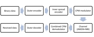
Figure II.1: A block diagram of the spread coded CPM system.

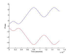
Figure II.2: An example GFSK signal’s phase under the two possible spread codes at a given location.

III Asymptotic performance of demodulation

We proceed to state the main results of the paper, comparing the performance of the two demodulation approaches. The proofs of the theorems in this section are deferred to Appendix B. We make several simplifying assumptions to allow for a tractable mathematical theory of asymptotic bit error rates. We assume that the symbol sequence $B$ is binary, so that the code words at any given bit position are just complements of each other and have a simple distance structure. We also assume that the code words are formed from a repetition-like code, which results in periodic distances between CPM signals, and that the background is additive Gaussian white noise, which leads to explicit symbolic formulas for error probabilities in signal classification (see Appendix A). However, our results allow for arbitrary CPM pulse shapes, such as GFSK or raised cosine (RC) pulses.

Our first result establishes sharp asymptotic bounds on the distance between two complemented binary CPM waveforms, as would be the case in a repetition code, over an observation interval of $N$ symbols. For any functions $f$ and $g$, we use the Landau notation $f(N)\sim g(N)$ to denote $f(N)/g(N)\to 1$ as $N\to\infty$.

Theorem 1.

For any binary symbol sequence $B$ ending with $N$ identical symbols, let $B^{\prime}$ be the same sequence with those $N$ symbols flipped. Let $s_{B}$ and $s_{B^{\prime}}$ be the corresponding CPM signals given by (II.1). Assume that $F$ is zero outside $[-1,1]$ and that $F(t)=F(-t)$. As $N\to\infty,$

$$\lim_{\omega_{c}\to\infty}\left\|s_{B}-s_{B^{\prime}}\right\|_{L^{2}(0,N)}\sim\sqrt{2N},$$ (III.1)

and for the complex-analytic signals $P^{+}s_{B}$ and $P^{+}s_{B^{\prime}}$ with $\cos(\cdot)$ in (II.1) replaced by $2^{-1/2}\exp(i\cdot)$,

$$\lim_{\omega_{c}\to\infty}\left\|P^{+}s_{B}-P^{+}s_{B^{\prime}}\right\|_{L^{2}(0,N)}\sim\sqrt{2N},$$ (III.2)

$$\lim_{\omega_{c}\to\infty}\frac{\left|\int_{0}^{N}P^{+}s_{B}(t)\overline{P^{+}s_{B^{\prime}}(t)}dt\right|}{\left\|P^{+}s_{B}\right\|_{L^{2}(0,N)}\left\|P^{+}s_{B^{\prime}}\right\|_{L^{2}(0,N)}}\sim\frac{E_{0}(N)}{\sqrt{2}N},$$ (III.3)

where $E_{0}$ is a function satisfying $|E_{0}(N)|\leq\frac{3}{2}\left(1+\frac{1}{h}\right)$ for all $N$.

Theorem 1 indicates that even when the CPM waveforms are not chosen to be orthogonal for any fixed $N$, such as e.g. binary MSK, they still become orthogonal in the limit as $N\to\infty$. In practice, the condition on $F$ can be relaxed to read that $F$ is “approximately” zero outside $[-1,1]$, as is the case with GFSK modulation, and the asymptotic bound still holds.

This result is used to compare the error probabilities of performing demodulation and decoding jointly, denoted by $p_{\mathrm{Joint}}^{\mathrm{NC}}$ and $p_{\mathrm{Joint}}^{\mathrm{C}}$ for noncoherent and coherent demodulation respectively, with that of doing them separately, denoted by $p_{\mathrm{Separate}}^{\mathrm{NC}}$ and $p_{\mathrm{Separate}}^{\mathrm{C}}$.

Theorem 2.

(Combined decoding and demodulation) Suppose the modulation is given by (II.1) with the constraints in Theorem III.1, and let $\omega_{c}\to\infty$. Then for a fixed noise power $\sigma^{2}$, as $N\to\infty$,

$$p_{\mathrm{Joint}}^{\mathrm{NC}}\sim\frac{1}{2}I_{0}\left(\frac{\sqrt{2}E_{0}(N)}{8\sigma^{2}}\right)e^{-\frac{N}{4\sigma^{2}}}\approx\frac{1}{2}e^{-\frac{N}{4\sigma^{2}}}$$

and

$$p_{\mathrm{Joint}}^{\mathrm{C}}\sim\frac{\sigma}{\sqrt{\pi N}}e^{-\frac{N}{4\sigma^{2}}}.$$

Here, $I_{0}$ is the modified Bessel function defined by $I_{0}(x)=\sum_{n=0}^{\infty}\frac{(x/2)^{2n}}{n!^{2}}$. In the noncoherent bound, the coefficient turns out to be very close to $\frac{1}{2}$ when $\sigma^{2}\geq 1$. In general, the function $E_{0}$ in (III.3) is oscillatory and it is not easy to characterize its behavior precisely, but it is typically between $0$ and $1$, and since $\frac{1}{2}I_{0}(x)\sim\frac{1}{2}+\frac{1}{8}x^{2}$ as $x\to 0$, the coefficient is about $\frac{1}{2}$.

Theorem 3.

(Separate decoding and demodulation) Suppose the modulation is given by (II.1) with the constraints in Theorem III.1, and let $\omega_{c}\to\infty$. Assume that $N$ is odd and $C=\lim_{\omega_{c}\to\infty}\left\|s_{\{0\}}-s_{\{1\}}\right\|_{L^{2}(0,1)}\leq\sigma$, i.e. the noise is at least as strong as the signal separation. Then for a fixed noise power $\sigma^{2}$ and for all sufficiently large $N$,

$$p_{\mathrm{Separate}}^{\mathrm{NC}}\geq\frac{\left(e^{-1/8}\left(2-e^{-1/8}\right)\right)^{\frac{N+1}{2}}}{\sqrt{2\pi N}\left(1-\frac{1}{2}e^{-1/8}\right)}\approx\frac{0.71}{\sqrt{N}}\times 0.993^{N+1}$$

and

$$p_{\mathrm{Separate}}^{\mathrm{C}}\geq\frac{1}{\sqrt{N}}\left(1-\frac{1}{2\pi}\right)^{\frac{N+1}{2}}\approx\frac{1}{\sqrt{N}}0.917^{N+1}.$$

The distance $C$ in Theorem 3 can be calculated explicitly for certain shaping functions $F$. For binary, orthogonal FSK with $\mathrm{MI}=1$, it is easy to check that $C=\sqrt{2}$ and that the exponents in Theorem 2 become $0.882$ under the same restriction $C\leq\sigma$. These results can also be formulated in terms of the symbol-to-noise ratio $E_{s}/N_{0}$ instead of the noise power $\sigma^{2}$, using the equivalence $E_{s}/N_{0}=\frac{1}{4\sigma^{2}}\left\|s_{\{0\}}-s_{\{1\}}\right\|_{L^{2}}^{2}$ for CPM signals [1]. Theorem 3 holds when $E_{s}/N_{0}\leq\frac{1}{4}=-6\,\mathrm{dB}$.

Theorems 2 and 3 together show that as $N\to\infty$, $p_{\mathrm{Joint}}^{\mathrm{NC}}$ and $p_{\mathrm{Joint}}^{\mathrm{C}}$ decay significantly faster than $p_{\mathrm{Separate}}^{\mathrm{NC}}$ and $p_{\mathrm{Separate}}^{\mathrm{C}}$ for high noise power $\sigma^{2}$, with a much bigger difference in the noncoherent case. Note that these estimates are quite conservative when the demodulation is performed over multiple data bits at a time, taking advantage of the symbol memory inherent in CPM, but they serve to illustrate the improvement of the combined approach over the separated approach. We also point out that $p_{\mathrm{Joint}}^{\mathrm{C}}$ and $p_{\mathrm{Joint}}^{\mathrm{NC}}$ are of similar order and only differ by an $N^{-1/2}$ factor, while $p_{\mathrm{Separate}}^{\mathrm{C}}$ is far smaller than $p_{\mathrm{Separate}}^{\mathrm{NC}}$. This is intuitively reasonable, since the longer noncoherent observation intervals in the combined approach make more use of the memory in a CPM signal and are comparable to accounting for the entire symbol history that led to the phase at the most recent symbol position.

IV Extensions and simulations

In this section, we discuss some extensions of the ideas in Section III and consider numerical Monte Carlo simulations of the demodulation approaches we have studied. Some plots comparing the spectral density of a DSSS spread coded CPM signal to that of uncoded and repetition coded signals are shown in Figure IV.1. As an illustrative example, we consider a $6$Mbit/sec GFSK signal formed from $4000$ random, equiprobable data bits and sampled at $30$Mbit/sec, with $N=10$, $h=0.8$ and $\mathrm{BT}=0.3$. These parameters are similar to the GMSK modulation used in GSM, but the higher modulation index results in a flatter spectral density shape over the main lobe. The spectral density is estimated using the multitaper method [29] and the spread coded spectrum appears slightly thicker due to the signal being ten times as long, but the overall shape is unchanged from the uncoded case and remains flat over the main lobe. The fixed length of the code word sequence means that the signal will still contain periodicities, but these will be at (baseband) frequencies that are too low to be detectable or relevant in practice. In our simulations, we assume that the code words are generated in advance and stored in memory at both the transmitter and receiver ends. Alternatively, a deterministic procedure such as a maximum-length shift register with a known initial state can be used to generate the code words in real-time at both ends. Both implementation approaches have essentially the same effect on the spectral density.

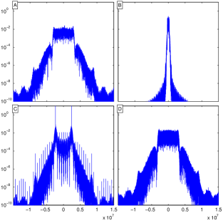
Figure IV.1: Spectral density profiles with (A) no coding applied, (B) no coding but with a reduced, $600$kbit/sec symbol rate, (C) repetition coding with rate $N=10$, and (D) spread coding with rate $N=10$.

In general, the distances between spread coded CPM waveforms may differ from the repetition case addressed by Theorem 1. Except in some special cases (e.g. when $h=1$), the periodicity techniques used to prove Theorem 1 (see Appendix B) no longer apply and the waveforms in (III.1) may no longer be approximately orthogonal. However, on average, we find that the results of Theorem 1 still hold in practice. In Figure IV.2, we numerically examine the distances for the modulation parameters discussed earlier at different rates $N$. We take all $2^{N}$ symbol sequences $B$ of length $N$ and calculate the mean of the distances $\left\|s_{B}-s_{B^{\prime}}\right\|_{L^{2}(0,N)}$ over all such $B$. It can be seen that for large $N$, this mean distance approaches the same $\sqrt{2N}$ limit established in Theorem 1.

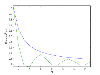
Figure IV.2: Mean distances over all $2^{N}$ spread coded waveforms (blue) at different rates $N$, compared to repetition coded waveforms (green).

We now study the performance of spread coding in simulations and compute the error rates for a range of code rates $N$. For the purposes of simulations, we use the method of noncoherent-block CPM demodulation over $K=5$ data bits (see [1] and [25, p. 298-299]) as a substitute for a fully coherent demodulator. At each bit position $a$, this demodulator takes a $K$-bit length of the received signal centered at $a$ and computes envelope correlators (see Appendix A) against all $2^{K}$ possible waveforms, outputting the bit $b$ at $a$ based on the average correlation over all waveforms containing $b$ at $a$. For $K\leq 7$, this approach exhibits performance similar to the optimal coherent (Viterbi-based) receiver, with rapidly diminishing gains for larger $K$, and is often used in practice for its low complexity and simple implementation. For such a demodulator, it is generally no longer possible to obtain precise asymptotic bounds of the type we developed in Section III for the special case $K=1$. However, any block code can be incorporated into this scheme by observing the signal over $NK$ symbols at a time but correlating it against only the $2^{K}$ possible waveforms, using knowledge of the underlying code (e.g. the pseudorandom code words). Hardware implementations of this scheme typically use $K=5$ or $7$, which allows the demodulation to be performed in close to real time. We use this approach in the results that follow.

In Figure IV.3, we use the same CPM parameters as before and examine the BER for different code rates $N$ at the noise levels given by $E_{s}/N_{0}=0\,\mathrm{dB}$ and $-3\,\mathrm{dB}$, with a uniformly distributed initial phase. We also compare the results with several standard convolutional codes of rates $1/N$ and constraint length $8$ [25, p. 492-494]. The results show that the spread code with combined, noncoherent-block demodulation greatly outperforms the other methods, especially in the $E_{s}/N_{0}=-3\,\mathrm{dB}$ case. At low $N$, the convolutional codes actually increase the BER over an uncoded signal and highlight the drawbacks of powerful, short-length codes in such noise environments, although as either $N$ or $E_{s}/N_{0}$ increase, we would expect such codes to eventually outperform the repetition-based spread codes. For moderate rates $N$, these results indicate that the spread codes have an “imperfectness” of $1-2$db under the combined demodulation approach, in terms of the lower bounds for codes of such rates discussed in [8], so it is not possible for a coding scheme to perform substantially better without using larger block lengths. We also note that the BERs obtained here are comparable to trellis coded noncoherent CPM schemes discussed in [33] or the baseline serially concatenated schemes described in [19] (the latter paper demonstrates much better BERs by inserting interleavers that are $2000$ or more symbols long, which effectively increases the block length and would be unsuitable for our design constraints as discussed in Section A).

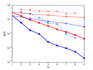
Figure IV.3: BER performance of CPM signals with spread coding using combined demodulation (bold curves) and separated demodulation (thin curves), along with convolutional coding (dashed curves), at $E_{s}/N_{0}=0\,\mathrm{dB}$ (blue) and $E_{s}/N_{0}=-3\,\mathrm{dB}$ (red).

We next compare the performance of a fixed rate spread code at different $E_{s}/N_{0}$, as well as in the presence of narrowband interference. We simulate a single $3$kbit/sec quadrature phase-shift keyed (QPSK) interferer at a random (but fixed) frequency within the band $\omega_{c}\pm 30$Mhz, which corresponds to the GFSK signal’s main lobe (see Figure IV.1), and with the same power as an equivalent level of white noise determined by the $E_{s}/N_{0}$. We take $N=6$ and plot the BERs of a spread coded CPM signal. We also consider the effects of changing the signal modulation to QPSK at the same data rate. The basic effect of the spread code increasing the distances between waveforms holds for QPSK as well, with the same $\sqrt{2N}$ asymptotic behavior as in Theorem III.1 for large $N$. Finally, we consider an example concatenating a rate $3$ spread coded CPM signal with a rate $1/2$ convolutional code at different error rates under white noise, which is how this technique is best applied in practice. The results are all shown in IV.4.

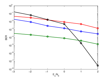
Figure IV.4: Performance of rate $6$ spread coded CPM under white noise (blue) and narrowband interference (green) using the combined demodulation approach. Also shown are rate $6$ spread coded QPSK under white noise (red) and rate $3$ spread coded and rate $1/2$ convolutional coded CPM under white noise (black).

V Conclusion

We have proved that combining the processes of decoding and demodulation with simple, DSSS-based and repetition-like coding schemes can confer significant advantages in high noise environments. We expect our results to generalize to broader classes of short-length block codes or other modulation schemes, as well as other demodulation approaches such as those that output soft symbol decisions and/or have observation intervals of multiple data bits. These topics will be pursued in future work.

Appendix A Background on signal classification theory

Before proving the Theorems 1-3, we first review some standard results on continuous-time binary signal classification from [24] and [31]. Let $f\in L^{2}(I)$ be a continuous, real deterministic function over some time interval $I$ and let $G$ be a Gaussian white noise process with power $\sigma^{2}$. Suppose we receive the (random) signal $Y(t)$ and want to determine which of the hypotheses $H_{0}=\{Y=G\}$ and $H_{1}=\{Y=f+G\}$ holds. The likelihood ratio test for this coherent classification problem is given by

$$e^{\frac{1}{\sigma^{2}}\left\langle f,Y\right\rangle_{I}-\frac{d^{2}}{2}}\lessgtr\tau.$$ (A.1)

where $\tau$ is a fixed threshold, $d=\frac{1}{\sigma}\left\|f\right\|_{L^{2}}$ and the inner product $\left\langle\cdot,Y\right\rangle_{I}$ is interpreted as a white noise functional. The performance of the test is given in terms of the error function $\mathrm{erf}(x)=2\pi{}^{-1/2}\int_{0}^{x}e^{-y^{2}}dy$ by

$$P(H_{1}|H_{1}) = \frac{1}{2}\mathrm{erf}\left(\frac{1}{\sqrt{2}}\left(\frac{\log\tau}{d}+\frac{d}{2}\right)\right)+\frac{1}{2},$$

$$P(H_{1}|H_{0}) = \frac{1}{2}\mathrm{erf}\left(\frac{1}{\sqrt{2}}\left(\frac{\log\tau}{d}-\frac{d}{2}\right)\right)+\frac{1}{2}.$$

We take $\tau=1$ and $f=f_{1}-f_{2}$, where $f_{1}$ and $f_{2}$ are known, modulated waveforms corresponding to a $0$ or $1$ bit. The test (A.1) reduces to a simple correlation classifier:

$$\left\langle f_{1},Y\right\rangle_{I}\lessgtr\left\langle f_{2},Y\right\rangle_{I}.$$ (A.2)

Assuming that $P(H_{0})=P(H_{1})$, the probability of a symbol classification error is

$$p = \frac{1}{2}-\frac{1}{2}\mathrm{erf}\left(\frac{\left\|f_{1}-f_{2}\right\|_{L^{2}(I)}}{2\sqrt{2}\sigma}\right).$$ (A.3)

Similar results can also be shown for noncoherent classification, where $f$ is now complex-valued and we instead have $H_{1}=\{Y=2^{1/2}\mathrm{Re}(e^{2\pi i\theta}f)+G\}$ for some unknown phase angle $\theta$. If $\theta$ is assumed to be random and uniformly distributed over $[0,1]$, the correlation classifier (A.2) is replaced by the envelope classifier given by

$$\left|\left\langle f_{1},Y\right\rangle_{I}\right|\lessgtr\left|\left\langle f_{2},Y\right\rangle_{I}\right|.$$

When $f_{1}$ and $f_{2}$ have equal norms, the error probability of this classifier is [25, p. 311]

$$p = e^{-\frac{1}{2}(u^{2}+v^{2})}\sum_{k=0}^{\infty}(u/v)^{k}I_{k}(uv)$$ (A.4)

$$-\frac{1}{2}e^{-\frac{1}{2}(u^{2}+v^{2})}I_{0}(uv),$$

where

$$u = \frac{\left\|f_{1}-f_{2}\right\|_{L^{2}(I)}}{2\sqrt{2}\sigma}\left(1-\sqrt{1-\left|R_{I}(f_{1},f_{2})\right|^{2}}\right)^{1/2},$$

$$v = \frac{\left\|f_{1}-f_{2}\right\|_{L^{2}(I)}}{2\sqrt{2}\sigma}\left(1+\sqrt{1-\left|R_{I}(f_{1},f_{2})\right|^{2}}\right)^{1/2},$$

$$R_{I}(f_{1},f_{2})=\frac{\left\langle f_{1},f_{2}\right\rangle_{I}}{\left\|f_{1}\right\|_{L^{2}(I)}\left\|f_{2}\right\|_{L^{2}(I)}},$$

and $I_{k}(x)=\sum_{n=0}^{\infty}\frac{(x/2)^{2n+k}}{n!(n+k)!}$ is the modified Bessel function of order $k$. The probability (A.4) is minimized when $R_{I}(f_{1},f_{2})=0$ [28], in which case (A.4) simplifies to

$$p=\frac{1}{2}e^{-\frac{1}{8\sigma^{2}}\left\|f_{1}-f_{2}\right\|_{L^{2}(I)}^{2}}.$$ (A.5)

We also note that the error function in (A.3) satisfies the elementary bounds

$$\mathrm{erf}(x)\leq\frac{2x}{\sqrt{\pi}}$$ (A.6)

for $x\geq 0$ and

$$\mathrm{erf}(x)\sim 1-\frac{e^{-x^{2}}}{\sqrt{\pi}x}$$ (A.7)

as $x\to\infty$.

Appendix B Proof of Theorems 1-3

Proof of Theorem 1.

Let $s_{B,\theta_{0}}(t)$ be (II.1) with the phase $\theta$ replaced by $\theta+\theta_{0}$, where $\theta_{0}$ is either $0$ or $\frac{1}{4}$. The purpose of this extra parameter will become clear later. We also define $J(N,t)=\sum_{k=0}^{N}\int_{-\infty}^{t}F(s-k)ds$ to simplify some notation. First, we have

$$\left\|s_{B,\theta_{0}}-s_{B^{\prime}}\right\|_{L^{2}(0,N)}^{2}$$

$$= \left\|s_{B,\theta_{0}}\right\|_{L^{2}(0,N)}^{2}+\left\|s_{B^{\prime}}\right\|_{L^{2}(0,N)}^{2}-2\left\langle s_{B,\theta_{0}},s_{B^{\prime}}\right\rangle_{(0,N)}$$

$$= 2N-E_{1}(\omega_{c})-2\int_{0}^{N}\cos\bigg{(}2\pi\bigg{(}\theta_{0}+\frac{h}{2}\times$$

$$\sum_{k=-\infty}^{N}(2b_{k}-1-2b_{k}^{\prime}+1)\int_{-\infty}^{t}F(s-k)ds\bigg{)}\bigg{)}dt$$

$$= 2\int_{0}^{N}\left(1-\cos\left(2\pi\left(\theta_{0}+h\,J(N,t)\right)\right)\right)dt$$ (B.1)

$$\quad-E_{1}(\omega_{c}),$$

where $E_{1}(\omega_{c})=O(1/\omega_{c})$. Taking $\omega_{c}\to\infty$ causes this term to drop out. Now the function $1-\cos(2\pi x)$ is well approximated by a sum of hat functions $2\sum_{m=-\infty}^{\infty}H(x-m)$, where the hat function $H(x)$ is given by $H(x)=2x$ for $x\in[0,\frac{1}{2})$, $H(x)=2-2x$ for $x\in[\frac{1}{2},1)$, and $H(x)=0$ otherwise. We define the approximation error

$$E_{2}(x)=2\sum_{m=-\infty}^{\infty}H(x-m)-(1-\cos(2\pi x)).$$

$E_{2}(x)$ is periodic with period $1$ and satisfies $|E_{2}(x)|\leq\frac{1}{4}$ and $E_{2}(x)=-E_{2}(\frac{1}{2}-x)=E_{2}(1-x)$ (see Figure B.1), which implies that $\int_{0}^{M}E_{2}(x+\frac{1}{2})dx=0$ for any $M\in\mathbb{Z}$. The conditions on $F$ show that $J(N,\cdot)$ is a continuous, nondecreasing function that equals $t+\frac{1}{2}$ for $t\in\mathbb{Z}\cap[0,N]$. This shows that as long as $N\geq\frac{1}{h}$, there exists a point $M^{\prime}\leq N$ with $\left|M^{\prime}-N\right|\leq\frac{1}{h}$ such that

$$\int_{0}^{M^{\prime}}E_{2}\left(\theta_{0}+h\,J(N,t)\right)dt=0.$$

Now let $A\leq 0$ be the closest point to $0$ such that $h\,J(N,A)=0$, and let $B\geq N-\frac{1}{h}$ be the closest point to $N$ such that $h\,J(N,B)-\frac{1}{2}\in\mathbb{Z}$. Since $F$ is identically zero outside $[-1,1]$, we must have $A\geq-1$ and $B\leq N+\frac{1}{2}$. We can use this to find that as $N\to\infty$,

$$2\int_{0}^{N}\left(1-\cos\left(2\pi\left(\theta_{0}+h\,J(N,t)\right)\right)\right)dt$$

$$= 4\int_{0}^{N}\sum_{m=-\infty}^{\infty}H\left(\theta_{0}+h\,J(N,t)-m\right)dt-$$

$$\quad 2\int_{0}^{N}E_{2}\left(\theta_{0}+h\,J(N,t)\right)dt$$

$$\sim 4\int_{A}^{B}\sum_{m=-\infty}^{\infty}H\left(\theta_{0}+h\,J(N,t)-m\right)dt-$$

$$\quad 2\int_{M^{\prime}}^{N}E_{2}\left(\theta_{0}+h\,J(N,t)\right)dt$$

$$\sim 4\cdot\frac{B-A}{2}+E_{0}(N)$$

$$\sim 2N,$$

where $E_{0}(N)=2\int_{M^{\prime}}^{N}E_{2}\left(\theta_{0}+h\,J(N,t)\right)dt$ satisfies the bound $|E_{0}(N)|\leq 2(-A-(B-N))+\frac{N-M^{\prime}}{2}\leq\frac{3}{2}\left(1+\frac{1}{h}\right)$. Taking $\theta_{0}=0$ completes the proof. For the complex case (III.2), we simply replace $\theta$ by $\theta+\frac{1}{4}$ and obtain the same bound for the quadrature signal $s_{B}^{\star}$ with $\cos(\cdot)$ in (II.1) replaced by $\sin(\cdot)$, and therefore also for the analytic signal $P^{+}s_{B}=2^{-1/2}(s_{B}+is_{B}^{\star})$. Finally, for the inner product estimate (III.3), we first take $\theta_{0}=0$ to get

$$\mathrm{Re}\left(R_{(0,N)}(P^{+}s_{B},P^{+}s_{B^{\prime}})\right)$$

$$= \frac{\left\|P^{+}s_{B}\right\|_{L^{2}(0,N)}^{2}+\left\|P^{+}s_{B^{\prime}}\right\|_{L^{2}(0,N)}^{2}}{2\left\|P^{+}s_{B}\right\|_{L^{2}(0,N)}\left\|P^{+}s_{B^{\prime}}\right\|_{L^{2}(0,N)}}$$

$$\quad-\frac{\left\|P^{+}s_{B}-P^{+}s_{B^{\prime}}\right\|_{L^{2}(0,N)}^{2}}{2\left\|P^{+}s_{B}\right\|_{L^{2}(0,N)}\left\|P^{+}s_{B^{\prime}}\right\|_{L^{2}(0,N)}}$$

$$\sim \frac{E_{0}(N)}{2N}.$$

By taking $\theta_{0}=\frac{1}{4}$, the same result follows for $\mathrm{Im}\left(R_{(0,N)}(P^{+}s_{B},P^{+}s_{B^{\prime}})\right)$, and thus

$$\left|R_{(0,N)}(P^{+}s_{B},P^{+}s_{B^{\prime}})\right|\sim\frac{E_{0}(N)}{\sqrt{2}N}.$$

∎

   

Figure B.1: The approximation error $E_{2}$.

Proof of Theorem 2.

The coherent result follows immediately from combining (A.3) and (III.1). As $N\to\infty$, we use (A.7) to find that

$$p_{\mathrm{Joint}}^{\mathrm{C}} \sim \frac{1}{2}-\frac{1}{2}\mathrm{erf}\left(\frac{\sqrt{2N}}{2\sqrt{2}\sigma}\right).$$

$$\sim \frac{1}{2}-\frac{1}{2}\left(1-\frac{e^{-\left(\frac{\sqrt{2N}}{2\sqrt{2}\sigma}\right)^{2}}}{\sqrt{\pi}\left(\frac{\sqrt{2N}}{2\sqrt{2}\sigma}\right)}\right)$$

$$= \frac{\sigma}{\sqrt{\pi N}}e^{-\frac{N}{4\sigma^{2}}}.$$

The noncoherent case uses the “almost orthogonality” implied by (III.3) to show that (A.4) is closely approximated by (A.5). Letting $\delta_{0,k}=1$ for $k=0$ and $\delta_{0,k}=0$ otherwise, we use (III.2) and (III.3) in (A.4) to get

$$p_{\mathrm{Joint}}^{\mathrm{NC}}$$ (B.3)

$$= e^{-\frac{1}{2}(u^{2}+v^{2})}\sum_{k=0}^{\infty}\left(1-\frac{\delta_{0,k}}{2}\right)(u/v)^{k}I_{k}(uv)$$

$$= e^{-\frac{1}{8\sigma^{2}}\left\|P^{+}s_{B}-P^{+}s_{B^{\prime}}\right\|_{L^{2}(0,N)}^{2}}\sum_{k=0}^{\infty}\left(1-\frac{\delta_{0,k}}{2}\right)\times$$

$$\quad\left(\frac{1-\sqrt{1-\left|R_{(0,N)}(P^{+}s_{B},P^{+}s_{B^{\prime}})\right|^{2}}}{1+\sqrt{1-\left|R_{(0,N)}(P^{+}s_{B},P^{+}s_{B^{\prime}})\right|^{2}}}\right)^{k/2}\times$$

$$\quad I_{k}\left(\frac{1}{8\sigma^{2}}\frac{\left\|P^{+}s_{B}-P^{+}s_{B^{\prime}}\right\|_{L^{2}(0,N)}^{2}}{\left|R_{(0,N)}(P^{+}s_{B},P^{+}s_{B^{\prime}})\right|^{-1}}\right)$$

$$\sim \sum_{k=0}^{\infty}\left(1-\frac{\delta_{0,k}}{2}\right)\left(\frac{1-\sqrt{1-E_{0}(N)/(4N^{2})}}{1+\sqrt{1-E_{0}(N)/(4N^{2})}}\right)^{k/2}$$

$$\quad\times I_{k}\left(\frac{\sqrt{2}E_{0}(N)}{8\sigma^{2}}\right)e^{-\frac{N}{4\sigma^{2}}}.$$

Using the basic property $\left|I_{k}(x)\right|\geq\left|I_{k+1}(x)\right|$ for each $k\geq 1$ [32], we conclude that as $N\to\infty$, all terms in the sum (B.3) go to zero uniformly in $k$ except for the $k=0$ term, which goes to $\frac{1}{2}I_{0}\left(\frac{\sqrt{2}E_{0}(N)}{8\sigma^{2}}\right)e^{-\frac{N}{4\sigma^{2}}}$. Consequently, we end up with

$$p_{\mathrm{Joint}}^{\mathrm{NC}} \sim \frac{1}{2}I_{0}\left(\frac{\sqrt{2}E_{0}(N)}{8\sigma^{2}}\right)e^{-\frac{N}{4\sigma^{2}}}.$$

∎

   

Proof of Theorem 3.

If $p$ is the error probability in demodulating an individual symbol, the error probability in a majority vote decoder is given by

$$p^{\prime}=\sum_{k=(N+1)/2}^{N}\frac{N!}{k!(N-k)!}p^{k}(1-p)^{N-k}.$$ (B.4)

For large $N$, we can approximate this using a classical extension of the Stirling expansion for the gamma function,

$$\Gamma(N+k+1)=\sqrt{2\pi}N^{N+k+\frac{1}{2}}e^{-N+E_{3}(N,k)},$$

with the error $E_{3}$ satisfying

$$\frac{1}{N+1}\leq\frac{E_{3}(N,k)}{\frac{k^{2}}{2}-\frac{k}{2}+\frac{1}{12}}\leq\frac{1}{N}$$

for $N\geq k>0$ [32]. This can be applied to (B.4) to obtain a simple geometric series after some simplification:

$$p^{\prime}$$

$$= \sum_{k=0}^{(N-1)/2}\frac{\Gamma(N+1)}{\Gamma(\frac{N+1}{2}+k+1)\Gamma(\frac{N-1}{2}-k+1)}\times$$

$$\quad p^{\frac{N+1}{2}+k}(1-p)^{\frac{N-1}{2}-k}$$

$$\sim \sum_{k=0}^{(N-1)/2}\frac{N^{N+\frac{1}{2}}e^{-N}p^{\frac{N+1}{2}+k}(1-p)^{\frac{N-1}{2}-k}}{(\frac{N+1}{2})^{\frac{N+1}{2}+k+\frac{1}{2}}(\frac{N-1}{2})^{\frac{N-1}{2}-k+\frac{1}{2}}e^{-N}}$$

$$\quad\times(2\pi)^{-1/2}e^{E_{3}(N,k)-E_{3}(\frac{N+1}{2},k)-E_{3}(\frac{N-1}{2},-k)}$$

$$\sim \frac{N^{N+\frac{1}{2}}p^{\frac{N+1}{2}}(1-p)^{\frac{N-1}{2}}}{\sqrt{2\pi}(\frac{N+1}{2})^{\frac{N+1}{2}+\frac{1}{2}}(\frac{N-1}{2})^{\frac{N-1}{2}+\frac{1}{2}}}\times$$

$$\quad\sum_{k=0}^{\infty}\left(\frac{4p}{\left(N^{2}-1\right)(1-p)}\right)^{k}\times$$

$$\quad e^{-\frac{1}{N}\left(\frac{(3N^{2}+1)(k^{2}+1/6)+(N^{2}+4N-1))k}{2(N^{2}-1)}\right)}$$

$$\sim \frac{(2N)^{N+\frac{1}{2}}(p(1-p))^{\frac{N+1}{2}}}{(N^{2}-1)^{\frac{N}{2}}((1-2p)N+1)\sqrt{\pi}}$$

$$= \frac{(4p(1-p))^{\frac{N+1}{2}}}{\sqrt{2\pi}((1-2p)\sqrt{N}+1/\sqrt{N})},$$ (B.6)

where in (B), we used the fact that the exponential factor in the sum tends uniformly to $1$ for all $k$. For the noncoherent case, we obtain a lower bound on the overall BER by assuming $\left\langle P^{+}s_{\{0\}},P^{+}s_{\{1\}}\right\rangle=0$, so that (A.5) applies, and using (III.2) and the condition $C\leq\sigma$. The function $e^{-x}(2-e^{-x})$ is decreasing for $x>0$, so for sufficiently large $N$,

$$p_{\mathrm{Separate}}^{\mathrm{NC}}$$

$$\geq \frac{\left(4\left(\frac{1}{2}e^{-C^{2}/(8\sigma^{2})}\right)\left(1-\frac{1}{2}e^{-C^{2}/(8\sigma^{2})}\right)\right)^{\frac{N+1}{2}}}{\sqrt{2\pi N}\left(1-\frac{1}{2}e^{-C^{2}/(8\sigma^{2})}\right)}$$

$$\geq \frac{\left(e^{-1/8}\left(2-e^{-1/8}\right)\right)^{\frac{N+1}{2}}}{\sqrt{2\pi N}\left(1-\frac{1}{2}e^{-1/8}\right)}.$$

In the coherent case, the error probabilities $p$ at consecutive symbols from the demodulator are no longer independent, but we can again find a lower bound on the BER by considering a best-case scenario where at any symbol position, all previous symbols were demodulated correctly and the initial phase is thus known. For sufficiently large $N$, we use the estimate (III.1) with (B.6) to get

$$p_{\mathrm{Separate}}^{\mathrm{C}}$$

$$\geq \frac{\left(4\left(\frac{1}{2}-\frac{1}{2}\mathrm{erf}\left(\frac{C}{2\sqrt{2}\sigma}\right)\right)\left(-\frac{1}{2}+\frac{1}{2}\mathrm{erf}\left(\frac{C}{2\sqrt{2}\sigma}\right)\right)\right)^{\frac{N+1}{2}}}{\sqrt{2\pi N}\mathrm{erf}\left(\frac{C}{2\sqrt{2}\sigma}\right)}$$

$$= \frac{1}{\sqrt{2\pi N}\mathrm{erf}\left(\frac{C}{2\sqrt{2}\sigma}\right)}\left(1-\mathrm{erf}\left(\frac{C}{2\sqrt{2}\sigma}\right)^{2}\right)^{\frac{N+1}{2}}.$$

Since $C\leq\sigma$, we take the inequality (A.6) into account and obtain

$$p_{\mathrm{Separate}}^{\mathrm{C}}$$

$$\geq \frac{1}{\sqrt{2\pi N}\left(\frac{C}{\sqrt{2\pi}\sigma}\right)}\left(1-\left(\frac{C}{\sqrt{2\pi}\sigma}\right)^{2}\right)^{\frac{N+1}{2}}$$

$$\geq \frac{1}{\sqrt{N}}\left(1-\frac{1}{2\pi}\right)^{\frac{N+1}{2}}.$$

∎

References

- [1] J. B. Anderson, T. Aulin, and C.-E. Sundberg. Digital Phase Modulation. Kluwer, 1986.
- [2] J. B. Anderson and C. E. Sundberg. Advances in Constant Envelope Coded Modulation. IEEE Communications Magazine, 29(12):36–45, 1991.
- [3] D. K. Asano, T. Hayashi, and R. Kohno. Modulation and processing gain tradeoffs in DS-CDMA spread spectrum systems. IEEE 5th International Symposium on Spread Spectrum Techniques and Applications, 1:9–13, 1998.
- [4] A. Barbieri and G. Colavolpe. Simplified soft-output detection of CPM signals over coherent and phase noise channels. IEEE Transactions on Wireless Communications, 6:2486–2496, 2007.
- [5] A. Barbieri, D. Fertonani, and G. Colavolpe. Spectrally-efficient continuous phase modulations. IEEE Transactions on Wireless Communications, 8:1564–1572, 2009.
- [6] G. Colavolpe and R. Raheli. Reduced-complexity detection and phase synchronization of CPM signals. IEEE Transactions on Communications, 45(9):1070–1079, 1997.
- [7] G. Colavolpe and R. Raheli. Noncoherent sequence detection of continuous phase modulations. IEEE Transactions on Communications, 47:1303–1307, 1999.
- [8] S. Dolinar, D. Divsalar, and F. Pollara. Code performance as a function of block length. TMO Progress Report 42-133, NASA JPL, 1998.
- [9] S. Dolinar, D. Divsalar, and F. Pollara. Turbo Code Performance as a Function of Code Block Size. Proc. IEEE International Symposium on Information Theory, 1998.
- [10] J. P. Fonseka. Block encoding with continuous phase modulation. IEEE Transactions on Communications, 42(12):3069–3072, 1994.
- [11] The Consultative Committee for Space Data Systems. Flexible serially concatenated convolutional turbo codes with near-Shannon bound performance for telemetry applications, experimental specification. 2007.
- [12] A. Graell i Amat, C.A. Nour, and C. Douillard. Serially Concatenated Continuous Phase Modulation with Extended BCH Codes. 2007 IEEE Workshop on Information Theory for Wireless Networks, pages 1–5, 2007.
- [13] A. Jamin and P. Mahonen. Wavelet packet modulation for wireless communications. Wireless Communications and Mobile Computing, 5(2):123–127, 2005.
- [14] W. Lane. Spread Spectrum Multi-h Modulation. Ph.D. Thesis, Georgia Institute of Technology, 1988.
- [15] A. R. Lindsey. Wavelet packet modulation for orthogonally multiplexed communication. IEEE Transactions on Signal Processing, 45(5):1336–1339, 1997.
- [16] T. M. Lok and J. S. Lehnert. DS/SSMA communication system with trellis coding and CPM. IEEE Journal on Selected Areas in Communications, 12(4):716–722, 1994.
- [17] N. Mazzali, G. Colavolpe, and S. Buzzi. CPM-based spread spectrum systems for multi-user communications. IEEE Transactions on Wireless Communications, 12:358–367, 2013.
- [18] U. Mengali and M. Morelli. Decomposition of M-ary CPM Signals into PAM Waveforms. IEEE Transactions on Information Theory, 41(5):1265–1275, 1995.
- [19] P. Moqvist and T. M. Aulin. Serially concatenated continuous phase modulation with iterative decoding. IEEE Transactions on Communications, 49:1901–1915, 2001.
- [20] P. Moqvist and T. M. Aulin. Orthogonalization by principal components applied to CPM. IEEE Transactions on Communications, 51(11):1838–1845, 2003.
- [21] F. Morales-Moreno and S. Pasupathy. Convolutional codes and MSK modulation: a combined optimization. Proc. 12th Biennial Sympopsium on Communications, pages c1.4–c1.7, 1984.
- [22] K. R. Narayanan and G. L. Stuber. Performance of Trellis-coded CPM with Iterative Demodulation and Decoding. IEEE Transactions on Communications, 49(4):676–687, 2001.
- [23] S. S. Pietrobon, R. H. Deng, A. Lafanechere, G. Ungerboeck, and D.J. Costello. Trellis-coded multidimensional phase modulation. IEEE Transactions on Information Theory, 36(1):63–89, 1990.
- [24] H. V. Poor. An Introduction to Signal Detection and Estimation. Springer, 1994.
- [25] J. G. Proakis. Digital Communications, Fourth Ed. McGraw-Hill, 2000.
- [26] B. E. Rimoldi. A decomposition approach to CPM. IEEE Transactions on Information Theory, 36(2):260–270, 1988.
- [27] P. J. Schreier, L. L. Scharf, and C. T. Mullis. Detection and Estimation of Improper Complex Random Signals. IEEE Transactions on Information Theory, 51(1), 2005.
- [28] Y. Sun, A. Baricz, and S. Zhou. On the monotonicity, log-concavity and tight bounds of the generalized Marcum and Nuttall Q-functions. IEEE Transactions on Information Theory, 56(3):1166–1186, 2010.
- [29] D.J. Thomson. Spectrum estimation and harmonic analysis. Proceedings of the IEEE, 70:1055–1096, 1982.
- [30] G. Ungerboeck. Channel coding with multilevel/phase signals. IEEE Transactions on Information Theory, 28(1):55–67, 1982.
- [31] H. L. Van Trees. Detection, Estimation and Modulation Theory: Part I. Wiley, 2001.
- [32] E. T. Whittaker and G. H. Watson. A Course of Modern Analysis, Fourth Ed. Cambridge Math. Library. Cambridge Univ. Press, 1927.
- [33] L. Yiin and G. Stuber. Noncoherently detected trellis-coded partial response CPM on mobile radio channels. IEEE Transactions on Communications, 44(8):967–975, 1996.