Testing for nodal dependence in relational data matrices

Abstract

Relational data are often represented as a square matrix, the entries of which record the relationships between pairs of objects. Many statistical methods for the analysis of such data assume some degree of similarity or dependence between objects in terms of the way they relate to each other. However, formal tests for such dependence have not been developed. We provide a test for such dependence using the framework of the matrix normal model, a type of multivariate normal distribution parameterized in terms of row- and column-specific covariance matrices. We develop a likelihood ratio test (LRT) for row and column dependence based on the observation of a single relational data matrix. We obtain a reference distribution for the LRT statistic, thereby providing an exact test for the presence of row or column correlations in a square relational data matrix. Additionally, we provide extensions of the test to accommodate common features of such data, such as undefined diagonal entries, a non-zero mean, multiple observations, and deviations from normality. KEY WORDS:  Networks; Matrix normal; hypothesis testing; Maximum likelihood

1 Introduction

Networks or relational data among $m$ actors, nodes or objects are frequently presented in the form of an $m\times m$ matrix $Y=\left\{y_{ij}:1\leq i,j\leq m\right\}$, where the entry $y_{ij}$ corresponds to a measure of the directed relationship from object $i$ to object $j$. Such data are of interest in a variety of scientific disciplines: Sociologists and epidemiologists gather friendship network data to study social development and health outcomes among children (Fletcher et al.,, 2011; Pollard et al.,, 2010; Potter et al.,, 2012; Van De Bunt et al.,, 1999), economists study markets by analyzing networks of business interactions among companies or countries (Westveld and Hoff, 2011a, ; Lazzarini et al.,, 2001), and biologists study gene-gene interaction networks to better understand biological pathways (Bergmann et al.,, 2003; Stuart et al.,, 2003).

Often of interest in the study of such data is a description of the variation and similarity among the objects in terms of their relations. Similarities among rows and among columns in empirical networks have long been observed (Sampson,, 1968; Leskovec et al.,, 2008), leading to the development of statistical tools to summarize such patterns. CONCOR (CONvergence of iterated CORrelations) is an early example of a procedure that partitions the rows (or columns) of $Y$ into groups based on a summary of the correlations among the rows (or columns) of $Y$ (White et al.,, 1976; McQuitty and Clark,, 1968). The procedure yields a “blockmodel” of the objects, a representation of the original data matrix $Y$ by a smaller matrix that identifies relationships among groups of objects. While this algorithm is still commonly used (Lincoln and Gerlach,, 2004; Lafosse and Ten Berge,, 2006), it suffers from a lack of statistical interpretability (Panning,, 1982), as it is not tied to any particular statistical model or inferential goal.

Several model-based approaches presume the existence of a grouping of the objects such that objects within a group share a common distribution for their outgoing relationships. This is the notion of stochastic equivalence, and is the primary assumption of stochastic blockmodels, a class of models for which the probability of a relationship between two objects depends only on their individual group memberships (Holland et al.,, 1983; Wang and Wong,, 1987; Nowicki and Snijders,, 2001; Rohe et al.,, 2011). Airoldi et al., (2008) extend the basic blockmodel by allowing each object to belong to several groups. In this model the probability of a relationship between two nodes depends on all the group memberships of each object. This and other variants of stochastic blockmodels belong to the larger class of latent variable models, in which the probability distribution of the relationship between any two objects $i$ and $j$ depends on unobserved object-specific latent characteristics $z_{i}$ and $z_{j}$ (Hoff et al.,, 2002). Statistical models of this type all presume some form of similarity among the objects in the network. However, while such models are widely used and studied, no formal test for similarities among the objects in terms of their relations has been proposed.

Many statistical methods for valued or continuous relational data are developed in the context of normal statistical models. These include, for example, the widely-used social relations model (Kenny and La Voie,, 1984; Li and Loken,, 2002) and covariance models for multivariate relational data (Li,, 2006; Westveld and Hoff, 2011b, ; Hoff,, 2011). Additionally, statistical models for binary and ordinal relational data can be based on latent normal random variables via probit or other link functions (Hoff,, 2005, 2008). In this article we propose a novel approach to testing for similarities between objects in terms of the row and column correlation parameters of the matrix normal model. The matrix normal model consists of the multivariate normal distributions that have a Kronecker-structured covariance matrix (Dawid,, 1981). Specifically, we say that an $m\times m$ random matrix $Y$ has the mean-zero matrix normal distribution $N_{m\times m}(0,\Sigma_{\rm r},\Sigma_{\rm c})$ if ${\rm vec}\left(Y\right)\sim N_{m^{2}}\left(0,\Sigma_{\rm c}\otimes\Sigma_{\rm r}\right)$ where “vec” is the vectorization operator and “$\otimes$” denotes the Kronecker product. Under this distribution, the covariance between two relations $y_{ij}$ and $y_{kl}$ is given by ${\rm cov}\left(y_{ij},y_{kl}\right)=\Sigma_{{\rm r},ik}\Sigma_{{\rm c},jl}$. Furthermore, it is straightforward to show that

$$E\left[YY^{t}\right]=\Sigma_{\rm r}{\rm tr}\left(\Sigma_{\rm c}\right)\ \text{and}\ E\left[Y^{t}Y\right]=\Sigma_{\rm c}{\rm tr}\left(\Sigma_{\rm r}\right).$$

These identities suggest the interpretation of $\Sigma_{\rm r}$ and $\Sigma_{\rm c}$ as the covariance of the objects as senders of ties and as receivers of ties, respectively. In this article, we evaluate evidence for similarities between objects by testing for non-zero correlations in this matrix normal model. Specifically, we develop a test of

$$H_{0}:\ (\Sigma_{\rm r},\Sigma_{\rm c})\in\mathcal{D}_{+}^{m}\times\mathcal{D}_{+}^{m}\ \ \text{versus}\ H_{1}:\ (\Sigma_{\rm r},\Sigma_{\rm c})\in(\mathcal{S}_{+}^{m}\times\mathcal{S}_{+}^{m})\backslash(\mathcal{D}_{+}^{m}\times\mathcal{D}_{+}^{m})$$

where $\mathcal{D}_{+}^{m}$ is the set of $m\times m$ diagonal matrices with positive entries and $\mathcal{S}_{+}^{m}$ is the set of $m\times m$ positive definite symmetric matrices. Model $H_{0}$, which we call the Kronecker variance model, represents heteroscedasticity among the rows and the columns while still maintaining their independence. Model $H_{1}$, which we call the full Kronecker covariance model, allows for correlations between all of the rows and all the of columns. Rejection of the null of zero correlation would support further inference via a model that allowed for similarities among the objects, such as a stochastic blockmodel, some other latent variable model or the matrix normal model. Acceptance of the null would caution against fitting such a model in order to avoid spurious inferences.

This goal of evaluating the evidence for row or column correlation is in contrast to that of the existing testing literature for matrix normal distributions. This literature has focused on an evaluation of the null hypothesis that ${\rm cov}({\rm vec}(Y))=\Sigma_{\rm c}\otimes\Sigma_{\rm r}$ (our $H_{1}$) against an unstructured alternative (Roy and Khattree,, 2005; Mitchell et al.,, 2006; Lu and Zimmerman,, 2005; Srivastava et al.,, 2008). The tests proposed in this literature are likelihood ratio tests that, in the case of an $m\times m$ square matrix $Y$, require at least $n>m^{2}$ replications to estimate the covariance under the fully unstructured model. Such tests are not applicable to most relational datasets, which typically consist of at most a few observed relational matrices.

In the next section we derive a hypothesis test of $H_{0}$ versus $H_{1}$ in the context of the matrix normal model. We show that given a single observed relational matrix $Y$, the likelihood is bounded under both $H_{0}$ and $H_{1}$ and so a likelihood ratio test of $H_{0}$ against $H_{1}$ can be constructed. We further show how the null distribution of the test statistic can be approximated with an arbitrarily high precision via a Monte Carlo procedure. In Section 2.3 we extend these results to the general class of matrix variate elliptically contoured distributions. The power of the test in several different situations is evaluated in Section 3.

Although the development of our testing procedure is based on the mean-zero matrix normal distribution, it is straightforward to extend the test to several other scenarios commonly encountered in the study of relational data, including missing diagonal entries, non-zero mean structure, multiple heteroscedastic observations and binary networks. These extensions and two data examples are discussed in Section 4. A discussion follows in Section 5.

2 Likelihood ratio test

In this section we propose a likelihood ratio test (LRT) for evaluating the presence of correlations among the rows and correlations among the columns of a square matrix. The data matrix $Y$ is modeled as a draw from a mean zero matrix normal distribution $N_{m\times m}\left(0,\Sigma_{\rm r},\Sigma_{\rm c}\right)$. The parameter space under the null hypothesis $H_{0}$ is $\Theta_{0}=\mathcal{D}_{+}^{m}\times\mathcal{D}_{+}^{m}$, the space of all pairs of diagonal $m\times m$ matrices with positive entries. Under the alternative $H_{1}$, the parameter space is $\Theta_{1}=(\mathcal{S}_{+}^{m}\times\mathcal{S}_{+}^{m})\backslash(\mathcal{D}_{+}^{m}\times\mathcal{D}_{+}^{m})$, the collection of all pairs of positive definite matrices of dimension $m$ for which at least one is not diagonal. To derive the LRT statistic, we first obtain the maximum likelihood estimates (MLEs) under the unrestricted parameter space $\Theta=\Theta_{0}\cup\Theta_{1}$ and under the null parameter space $\Theta_{0}$. From these MLEs, we construct several equivalent forms of the LRT statistic. While the null distribution of the test statistic is not available in closed form, the statistic is invariant under diagonal rescalings of the data matrix $Y$, implying that the distribution of the statistic is constant as a function of $(\Sigma_{\rm r},\Sigma_{\rm c})\in\Theta_{0}$. This fact allows us to obtain null distributions and $p$-values via Monte Carlo simulation.

2.1 Maximum likelihood estimates

The density of a mean zero matrix normal distribution $N_{m\times m}(0,\Sigma_{\rm r},\Sigma_{\rm c})$ is given by

$$p\left(Y|\Sigma_{\rm r},\Sigma_{\rm c}\right) = \left(2\pi\right)^{-m^{2}/2}\left|\Sigma_{\rm c}\otimes\Sigma_{\rm r}\right|^{-1/2}\exp(-\tfrac{1}{2}{\rm tr}\left(\Sigma_{\rm r}^{-1}Y\Sigma_{\rm c}^{-1}Y^{t}\right)),$$

where “tr” is the matrix trace and “$\otimes$” is the Kronecker product. Throughout the article we will write $l\left(\Sigma_{\rm r},\Sigma_{\rm c};Y\right)$ as minus two times the log likelihood minus $m^{2}\log 2\pi$, hereafter referred to as the scaled log likelihood:

$$l\left(\Sigma_{\rm r},\Sigma_{\rm c};Y\right) = -2\log p\left(Y|\Sigma_{\rm r},\Sigma_{\rm c}\right)-m^{2}\log 2\pi={\rm tr}\left[\Sigma_{\rm r}^{-1}Y\Sigma_{\rm c}^{-1}Y^{t}\right]-\log\left|\Sigma_{\rm c}^{-1}\otimes\Sigma_{\rm r}^{-1}\right|.$$ (1)

We will state all the results in this paper in terms of $l\left(\Sigma_{\rm r},\Sigma_{\rm c};Y\right)$. For example, an MLE will be a minimizer of $l\left(\Sigma_{\rm r},\Sigma_{\rm c};Y\right)$ in $(\Sigma_{\rm r},\Sigma_{\rm c})$. The following result implies that if $Y$ is a draw from an absolutely continuous distribution on $\mathbb{R}^{m\times m}$, then the scaled likelihood is bounded from below, and achieves this bound on a set of nonunique MLEs:

Theorem 1.

If $Y$ is full rank then $l(\Sigma_{\rm r},\Sigma_{\rm c};Y)\geq m^{2}+m\log|YY^{t}/m|$ for all $(\Sigma_{\rm r},\Sigma_{\rm c})\in\Theta$, with equality if $\Sigma_{\rm r}=Y{\Sigma}_{\rm c}^{-1}Y^{t}/m$, or equivalently, $\Sigma_{\rm c}=Y^{t}{\Sigma}_{\rm r}^{-1}Y/m$.

Proof.

We first look for MLEs at the critical points of $l\left(\Sigma_{\rm r},\Sigma_{\rm c};Y\right)$. Setting derivatives of $l$ to zero indicates that critical points satisfy

$$\hat{\Sigma}_{\rm r} = Y\hat{\Sigma}_{\rm c}^{-1}Y^{t}/m$$ (2)

$$\hat{\Sigma}_{\rm c} = Y^{t}\hat{\Sigma}_{\rm r}^{-1}Y/m.$$ (3)

Note that these equations are redundant: If $(\hat{\Sigma}_{\rm r},\hat{\Sigma}_{\rm c})$ satisfy Equation 2, then these values satisfy Equation 3 as well. The value of the scaled log likelihood at such a critical point is

$$l\left(Y\hat{\Sigma}_{\rm c}^{-1}Y^{t}/m,\hat{\Sigma}_{\rm c};Y\right) = {\rm tr}\left[\left(Y\hat{\Sigma}_{\rm c}^{-1}Y^{t}/m\right)^{-1}Y\hat{\Sigma}_{\rm c}^{-1}Y^{t}\right]+\log\left|\hat{\Sigma}_{\rm c}\otimes Y\hat{\Sigma}_{\rm c}^{-1}Y^{t}/m\right|$$ (4)

$$= m{\rm tr}\left[Y^{-t}\hat{\Sigma}_{\rm c}Y^{-1}Y\hat{\Sigma}_{\rm c}^{-1}Y^{t}\right]+m\log\left|\hat{\Sigma}_{\rm c}\right|-m\log\left|\hat{\Sigma}_{\rm c}\right|+m\log\left|YY^{t}/m\right|$$

$$= m{\rm tr}\left[I\right]+m\log\left|YY^{t}/m\right|.$$

In the second and third lines, $Y^{-1}$ exists and $|YY^{t}/m|>0$ since $Y$ is square and full rank. Now we compare the scaled log likelihood at a critical point to its value at any other point.

$$l\left(\Sigma_{\rm r},\Sigma_{\rm c};Y\right)-l(Y\hat{\Sigma}_{\rm c}^{-1}Y^{t}/m,\hat{\Sigma}_{\rm c};Y) =\text{tr}\left[\Sigma_{\rm r}^{-1}Y\Sigma_{\rm c}^{-1}Y^{t}\right]+m\log\left(\left|\Sigma_{\rm r}\right|\left|\Sigma_{\rm c}\right|\right)-m^{2}-m\log\left|YY^{t}/m\right|$$ (5)

$$=m^{2}\left[\frac{1}{m}\mbox{tr}\left[\Sigma_{\rm r}^{-1}Y\Sigma_{\rm c}^{-1}Y^{t}/m\right]-\frac{1}{m}\log\left|\Sigma_{\rm r}^{-1}Y\Sigma_{\rm c}^{-1}Y^{t}/m\right|-1\right]$$

The first equality is a simple combination of equations 1 and 4. The second equality is a rearrangement of terms that combines all the determinant in the log terms. This difference can be written as $m^{2}(a-\log g-1)$, where $a$ is the arithmetic mean and $g$ is the geometric mean of the eigenvalues of $(\Sigma_{\rm r}^{-1/2}Y\Sigma_{\rm c}^{-1}Y^{t}\Sigma_{\rm r}^{-1/2})/m$. To complete the proof we show that $a-\log g-1\geq 0$. Consider $f\left(x\right)=x-1-\log x$ and its first and second derivatives with respect to $x$: $f^{\prime}\left(x\right)=1-\frac{1}{x}$, and $f^{\prime\prime}\left(x\right)=\frac{1}{x^{2}}$. The second derivative is positive at the critical point $x=1$, so $f\left(1\right)=0$ is a global minimum of the function. Thus $x-\log x-1\geq 0$. Now let $\lambda_{1},\dots,\lambda_{m}$ be the eigenvalues of $(\Sigma_{\rm r}^{-1/2}Y\Sigma_{\rm c}^{-1}Y^{t}\Sigma_{\rm r}^{-1/2})/m$ and so $a=\frac{1}{m}\sum\lambda_{i}$ and $g=\left(\prod\lambda_{i}\right)^{1/m}$. We then have

$$a\geq\log a+1=\log\left(\frac{1}{m}\sum x_{i}\right)+1\geq\log\left(\left(\prod x_{i}\right)^{1/m}\right)+1=\log g+1$$

as $a\geq g$ since $\lambda_{i}\geq 0$ $\forall i$. Since $a-1-\log g\geq 0$ we have the desired result. ∎

Note that the MLE is not unique, nor is the MLE of $\Sigma_{\rm c}\otimes\Sigma_{\rm r}$. For example. $I\otimes YY^{t}/m$ is an MLE of $\Sigma_{\rm c}\otimes\Sigma_{\rm r}$, as is $Y^{t}Y\otimes I/m$. Moreover, there is an MLE for each $\Sigma_{\rm r}\in\mathcal{S}_{+}^{m}$ given by $(\Sigma_{\rm r},Y^{t}{\Sigma}_{\rm r}^{-1}Y/m)$, and similarly there is an MLE for each $\Sigma_{\rm c}\in\mathcal{S}_{+}^{m}$ given by $(Y\Sigma_{\rm c}^{-1}Y^{t}/m,\Sigma_{\rm c})$.

Theorem 1 also implies that the likelihood is bounded under the null. Unlike the unrestricted case, the MLE under the null is unique up to scalar multiplication:

Theorem 2.

If $Y$ is full rank then the MLE $\hat{D}_{\rm c}\otimes\hat{D}_{\rm r}$ under $H_{0}$ is unique, while $\hat{D}_{\rm r}$ and $\hat{D}_{\rm c}$ are unique up to a multiplication and division by the same positive scalar.

A proof is given in the Appendix. To find the MLE under the null model, we obtain the derivatives of the scaled log likelihood $l$ with respect to $(\Sigma_{\rm r},\Sigma_{\rm c})\in\Theta_{0}$. For notational convenience, we will refer to diagonal versions of $\Sigma_{\rm r}$ and $\Sigma_{\rm c}$ as $D_{\rm r}$ and $D_{\rm c}$ respectively. Setting these derivatives equal to zero, we establish that the critical points of $l$ must satisfy

$$D_{\rm r} = YD_{\rm c}^{-1}Y^{t}\circ I/m$$ (6)

$$D_{\rm c} = Y^{t}D_{\rm r}^{-1}Y\circ I/m$$ (7)

where “$\circ$” is the Hadamard product. The MLE can be found by iteratively solving equations (6) and (7). This procedure can be seen as a type of block coordinate descent algorithm, decreasing $l$ at each iteration (Tseng,, 2001).

2.2 Likelihood ratio test statistic and null distribution

Since the scaled log likelihood is bounded below, we are able to obtain a likelihood ratio statistic that is finite with probability 1 when $Y$ is sampled from an absolutely continuous distribution on $\mathbb{R}^{m\times m}$. As usual, a likelihood ratio test statistic can be obtained from the ratio of the unrestricted maximized likelihood to the likelihood maximized under the null. We take our test statistic to be

$$T(Y)=l(\hat{D}_{\rm r},\hat{D}_{\rm c};Y)-l(\hat{\Sigma}_{\rm r},\hat{\Sigma}_{\rm c};Y),$$

where $(\hat{\Sigma}_{\rm r},\hat{\Sigma}_{\rm c})$ is any unrestricted MLE and $(\hat{D}_{\rm r},\hat{D}_{\rm c})$ is the MLE under $\Theta_{0}$. Since the scaled log likelihood $l$ is minus two times the likelihood, our statistic is a monotonically increasing function of the likelihood ratio.

In Theorem 1 we showed that $l(\hat{\Sigma}_{\rm r},\hat{\Sigma}_{\rm c};Y)=m^{2}+m\log|YY^{t}/m|$ for any unrestricted MLE $(\hat{\Sigma}_{\rm r},\hat{\Sigma}_{\rm c})$. Similarly, letting $(\hat{D}_{\rm r},\hat{D}_{\rm c})$ be an MLE under $H_{0}$, we have

$$l(\hat{D}_{\rm r},\hat{D}_{\rm c};Y) ={\rm tr}\left[Y^{t}\hat{D}_{\rm r}^{-1}Y\hat{D}_{\rm c}^{-1}\right]+\log\left|\hat{D}_{\rm c}\otimes\hat{D}_{\rm r}\right|$$

$$={\rm tr}\left[(Y^{t}\hat{D}_{\rm r}^{-1}Y)(Y^{t}\hat{D}_{\rm r}^{-1}Y/m\circ I)^{-1}\right]+\log\left|\hat{D}_{\rm c}\otimes\hat{D}_{\rm r}\right|$$

$$=\sum_{i}(Y^{t}\hat{D}_{\rm r}^{-1}Y)_{ii}(Y^{t}\hat{D}_{\rm r}^{-1}Y/m\circ I)^{-1}_{ii}+\log\left|\hat{D}_{\rm c}\otimes\hat{D}_{\rm r}\right|$$

$$=m\sum_{i}(Y^{t}\hat{D}_{\rm r}^{-1}Y)_{ii}/(Y^{t}\hat{D}_{\rm r}^{-1}Y)_{ii}+\log\left|\hat{D}_{\rm c}\otimes\hat{D}_{\rm r}\right|=m^{2}+\log\left|\hat{D}_{\rm c}\otimes\hat{D}_{\rm r}\right|,$$

where the second equality stems from MLE satisfying $\hat{D}_{\rm c}=Y^{t}\hat{D}_{\rm r}^{-1}Y/m\circ I$ (Equation (7)). The third equality relies on the following identity for traces: for a diagonal matrix $A$ and unstructured matrix $B$ of the same dimension, ${\rm tr}\left[AB\right]=\sum_{i}A_{ii}B_{ii}$. The final line is due to the following identity for Hadamard products: if $I$ is the identity matrix and $B$ is an unstructured matrix, then $(B\circ I)^{-1}_{ii}=1/B_{ii}$.

The maximized likelihoods under the null and alternative give

$$T\left(Y\right) =\log\left|\hat{D}_{\rm c}\otimes\hat{D}_{\rm r}\right|-m\log\left|YY^{t}/m\right|$$

$$=m\left(\log\left|\hat{D}_{\rm c}\right|+\log\left|\hat{D}_{\rm r}\right|-\log\left|YY^{t}/m\right|\right).$$ (8)

Since no closed form solution exists for $\hat{D}_{\rm r}$ it is not clear how to obtain the null distributions of $T$ in closed form. However, it is possible to simulate from the null distribution of $T(Y)$, as the distribution of the test statistic is the same for all elements of the null hypothesis. To see this, we show that the test statistic itself is invariant under left and right transformations of the data by positive diagonal matrices. Let $\tilde{Y}=D_{1}YD_{2}$ for positive diagonal matrices $D_{1}$ and $D_{2}$. Since the MLE $\hat{D}_{\rm c}\otimes\hat{D}_{\rm r}$ is unique it is an equivariant function of any matrix $Y$ with respect to left and right multiplication by diagonal matrices (see Eaton, (1983) Prop 7.11). In particular, writing $\hat{\theta}\left(Y\right)$ for the estimate of $\hat{D}_{\rm c}\otimes\hat{D}_{\rm r}$ based on a data matrix $Y$, we have

$$\hat{\theta}\left(\tilde{Y}\right) = \left(D_{2}^{1/2}\otimes D_{1}^{1/2}\right)\hat{\theta}\left(Y\right)\left(D_{2}^{1/2}\otimes D_{1}^{1/2}\right).$$

Since the determinant is a multiplicative map, we can write the determinant of the above as

$$\left|\hat{\theta}\left(\tilde{Y}\right)\right| = \left|\left(D_{2}\otimes D_{1}\right)\right|\left|\hat{\theta}\left(Y\right)\right|.$$

Using the above, the $T\left(\tilde{Y}\right)$ can be written as in Equation (8):

$$T\left(\tilde{Y}\right) = m\log\left|\hat{\theta}\left(\tilde{Y}\right)\right|-m\log\left|\tilde{Y}\tilde{Y}^{t}/m\right|$$

$$= m\log\left|\hat{\theta}\left(Y\right)\right|+m\log\left|D_{2}\otimes D_{1}\right|-m\log\left|YY^{t}/m\right|-m\log\left|D_{2}\otimes D_{1}\right|=T\left(Y\right).$$

Since for a matrix normal random variable $Y\sim N_{m\times m}\left(0,\Sigma_{1},\Sigma_{2}\right)$ we have $Y\overset{d}{=}\Sigma_{1}^{1/2}Y_{0}\Sigma_{2}^{1/2}$ for $Y_{0}\sim N_{m\times m}\left(0,I,I\right)$, the above argument implies that $T\left(Y\right)\overset{d}{=}T\left(Y_{0}\right)$ under the null. Therefore, the null distribution of $T$ can be approximated via Monte Carlo simulation of $Y$ from any distribution in $H_{0}$. For example, a Monte Carlo approximation to the $q^{\rm th}$ quantile, $T_{q}$ can be obtained from the following algorithm:

1. Simulate $Y_{0}^{1},\dots,Y_{0}^{S}\sim\text{i.i.d}\ N_{m\times m}\left(0,I,I\right)$;

2. Let $\hat{T}_{q}=\min\{T(Y_{0}^{q}):\sum_{s=1}^{S}1[T(Y_{0}^{q})\geq T(Y_{0}^{s})]/S\geq q\}$.

2.3 Matrix variate elliptically contoured distributions

The results of the previous subsection are immediately extendable to the general class of matrix variate elliptically contoured distributions. In this section we show that under minor regularity conditions on the distributions, the likelihood for a matrix variate elliptically contoured distribution is bounded when the matrix normal distribution is bounded. We provide the form of an MLE for the general class of mean zero square matrix variate elliptically contoured distributions and demonstrate that the likelihood ratio test between $H_{0}$ and $H_{1}$ has the same form as in Equation (8).

We use the notation of Gupta and Varga, (1994) for the matrix variate elliptically contoured distribution. We say that $Y$ has a mean zero square matrix variate elliptically countoured distribution and write $Y\sim E_{m\times m}\left(0,\Sigma_{\rm r},\Sigma_{\rm c},h\right)$ if its density has the form

$$f_{Y}\left(Y\right)=\frac{1}{\left|\Sigma_{\rm r}\right|^{\frac{m}{2}}\left|\Sigma_{\rm c}\right|^{\frac{m}{2}}}h\left({\rm tr}\left[Y^{t}\Sigma_{\rm r}^{-1}Y\Sigma_{\rm c}^{-1}\right]\right)=\frac{1}{\left|\Sigma_{\rm r}\right|^{\frac{m}{2}}\left|\Sigma_{\rm c}\right|^{\frac{m}{2}}}h\left({\rm vec}\left(Y\right)^{t}\left(\Sigma_{\rm c}^{-1}\otimes\Sigma_{\rm r}^{-1}\right){\rm vec}\left(Y\right)\right).$$ (9)

For $h\left(w\right)=\left(2\pi\right)^{m^{2}/2}\exp\left(-\frac{1}{2}w\right)$, $Y$ is a mean zero matrix variate normal variable. Gupta and Varga, (1994) show that if $Y\sim E\left(0,\Sigma_{\rm r},\Sigma_{\rm c},h\right)$ then $AYB\sim E\left(0,A\Sigma_{\rm r}A^{t},B\Sigma_{\rm c}B^{t},h\right)$ and if second moments exist, then ${\rm cov}\left({\rm vec}\left(Y\right)\right)=c_{h}\left(\Sigma_{\rm c}\otimes\Sigma_{\rm r}\right)$. In Gupta and Varga, (1995), the authors showed that when $\Sigma_{\rm r}$ and $h$ are known, the MLE of $\Sigma_{\rm c}$ is proportional to the MLE of $\Sigma_{\rm c}$ under normality, but they do not provide results for the boundedness of the likelihood or existence of MLEs for the case where only $h$ is known. To find the form of the MLE in this case we state a simplified version of Theorem 1 of Anderson et al., (1986):

Theorem.

Let $\Omega$ be a set in the space of $\mathcal{S}_{+}^{m^{2}}$, such that if $V\in\Omega$ then $cV\in\Omega$ $\forall c>0$ (that is $\Omega$ is a cone). Suppose $h$ is such that $h\left(y^{t}y\right)$ is a density in $\mathbb{R}^{m^{2}}$ and $x^{m^{2}/2}h\left(x\right)$ has a finite positive maximum $x_{h}$. Suppose that on the basis of an observation $y$ from $\left|V\right|^{-1/2}h\left(y^{t}V^{-1}y\right)$ an MLE under normality $\tilde{V}\in\Omega$ exists and $\tilde{V}>0$ with probability 1. Then an MLE for $h$ is $\hat{V}=\left(m^{2}/x_{h}\right)\tilde{V}$ and the maximum of the likelihood is $\left|\hat{V}\right|^{-1/2}h\left(x_{h}\right)$.

In the previous subsection we proved that for the mean zero square matrix normal distribution, the likelihood is bounded for a single observation. A direct application of the above theorem with $\Omega=\mathcal{S}_{+}^{m}\times\mathcal{S}_{+}^{m}\subset\mathcal{S}_{+}^{m^{2}}$ and $y={\rm vec}\left(Y\right)$ proves that for the likelihood of a generic matrix variate elliptically contoured distribution with $h$ defined as in 9, the likelihood is bounded and the MLE of ${\rm cov}({\rm vec}(Y))$ is proportional to the MLE under normality. Clearly the theorem hold for a smaller space $\omega=\mathcal{D}_{+}^{m}\times\mathcal{D}_{+}^{m}\subset\mathcal{S}_{+}^{m^{2}}$ as well, and thus the likelihood ratio statistic can be constructed as follows

$$T\left(Y\right) =2\log\left[\left|\hat{V}_{\Omega}\right|^{-1/2}h\left(x_{h}\right)\right]-2\log\left[\left|\hat{V}_{\omega}\right|^{-1/2}h\left(x_{h}\right)\right]$$

$$=\log\left|\hat{V}_{\omega}\right|-\log\left|\hat{V}_{\Omega}\right|=\log|\tilde{V}_{\omega}|-\log|\tilde{V}_{\Omega}|$$ (10)

where $\tilde{V}_{\omega}$ and $\tilde{V}_{\Omega}$ are the MLEs under normality that were previously derived. Equation (10) is identical to the original form of the test (e.g. Equation (8)). As such, to conduct the test for any elliptically contoured distribtuion, we can construct a reference distribution for the null based on a mean zero matrix variate distribution.

3 Power calculations

In this section we present power calculations for three different types of covariance models. The three covariance models we consider are: (1) Exchangeable row covariance and exchangeable column covariance; (2) Maximally sparse Kronecker structured covariance; and (3) the covariance induced by a nonseparable stochastic blockmodel with two row groups and two column groups. For each covariance model, we consider the power as a function of parameters that control the total correlation within a covariance matrix as well as in terms of $m$, the dimension of the matrix. In Table 1 we present the 95% quantiles based on the null distributions required for performing level $\alpha=0.05$ tests.

Dimension $m$	5	10	15	20	25	30	50	100
95% quantile	43.3	144.3	297.4	502.8	760.0	1064.6	2802.1	10668.4

Table 1: 95% quantile of the null distribution of the test statistic for testing $H_{0}$ versus $H_{1}$. Approximation from 100,000 simulated values.

3.1 Exchangeable row and column covariance structure

We first consider a submodel of the matrix normal model in which $\Sigma_{\rm r}$ and $\Sigma_{\rm c}$ have exchangeable covariance structure. In this structure, the correlation between any two rows is a constant $\rho_{\rm r}$ and the correlation between any two columns is a constant $\rho_{\rm c}$. Specifically, ${\rm cov}({\rm vec}(Y))=\Sigma_{\rm c}\otimes\Sigma_{\rm r}$ where

$$\Sigma_{\rm r}=\left(1-\rho_{{\rm r}}\right)I+\rho_{{\rm r}}{\bf 11}^{t}\ \text{and}\ \Sigma_{\rm c}=\left(1-\rho_{{\rm c}}\right)I+\rho_{{\rm c}}{\bf 11}^{t},$$

and ${\bf 1}$ is a vector of ones of length $m$. We first consider a network with $m=10$ nodes and present the power as a function of $\rho_{\rm r}$ and $\rho_{\rm c}$ ranging from $-1/9$ to 1, where the lower bound guarantees that the covariance matrices are positive definite. We calculate the power on a $25\times 25$ grid in $[-1/9,1]^{2}$ and use a bivariate interpolation to construct the heatmap in the top left panel of Figure 1. From the plot it is evident that the power is an increasing function in $|\rho_{\rm r}|$ and $|\rho_{\rm c}|$. In particular, keeping $\rho_{\rm r}$ constant, the power is an increasing function of $|\rho_{\rm c}|$ and vice versa.

In the top left panel of Figure 1 we observed that while keeping $\rho_{\rm c}$ constant, the power is an increasing function of $|\rho_{\rm r}|$. To study the power for higher dimensional matrices, we set $\rho_{\rm c}=0$ and vary $m$ and $\rho_{\rm r}$. The dashed line in the top left panel of Figure 1 traces the power function for $m=10$ and $\rho_{\rm c}=0$. This corresponds to the same style dashed line in the top right hand panel of Figure 1. The other four lines in the right hand panel represent the calculated power as a function of $\rho_{\rm r}$ for different dimensions $m$, holding $\rho_{\rm c}=0$. As is expected, for each $m$, the power is an increasing function of $|\rho_{\rm r}|$. Similarly, for each fixed $\rho_{\rm r}$ value, the power is an increasing function of $m$. This latter phenomenon is due to the increase in the amount of data information with the increase in the dimension of the sociomatrix.

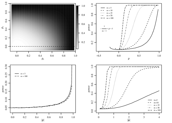
Figure 1: The top row of panels displays the power of the test under the exchangeable covariance model of Section 3.1. The bottom left panel displays the power of the test for the maximally sparse covariance model of Section 3.2 and the bottom right panel displays the power of the test for the nonseparable stochastic blockmodel of Section 3.3.

3.2 Maximally sparse Kronecker covariance structured correlation

While the previous example demonstrates the power of the test in the presence of many nonzero off-diagonal entries in the correlation matrices, it is of interest to see if the test has any power against alternatives that do not exhibit a large amount of correlation. For this purpose we consider a maximally sparse Kronecker covariance structure. We set the columns to be independent and only the first two rows to be correlated. This can be written compactly as $\Sigma_{\rm c}=I$ and $\Sigma_{\rm r}=I+\rho E_{12}+\rho E_{21}$, where $E_{ij}$ is the 0 matrix with a 1 in the $\left(i,j\right)^{\rm th}$ entry. For each of the matrix sizes $m\in\left\{5,10,25,50,100\right\}$ we computed power functions for values of $\rho$ ranging between -1 and 1. Monte Carlo approximations to the corresponding power functions are presented in the bottom left panel of Figure 1. We plot the results for $m=5$ and $m=100$ and see that the power increases monotonically as a function of $\left|\rho\right|$ for both dimensions. While the power of the test for a fixed $\rho$ appears to decrease as the size of the network $m$ increases, the two curves are nearly identical. We explain this as follows: while one expects that as the dimension $m$ increases there is an increase in data information for identifying the correlation $\rho$, the power curve is influenced more heavily by the fact that the difference between $\Sigma_{\rm r}$ and the identity matrix becomes less pronounced. Additional power curves for a range of $m$ values between 5 and 100 were approximated. All the curves were between the $m=5$ and $m=100$ curves that are presented in the plot. For all the power calculations, the lowest calculated power for values of $\rho$ close to 0 was always within two Monte Carlo standard errors of 0.05.

3.3 Misspecified covariance structure

In the Introduction we discussed a popular model for relational data with an underlying assumption of stochastically equivalent nodes called the stochastic blockmodel. Straightforward calculations show that in general the covariance induced by a stochastic blockmodel is nonseparable, but still induces correlations among the rows and among the columns. As such, we are interested in evaluating the power of our test against such nonseparable alternatives.

A stochastic blockmodel can be represented in terms of multiplicative latent variables. Specifically, we can write the relationship $y_{ij}=u_{i}^{t}Wv_{j}+\epsilon_{ij}$ where $u_{i}$ and $v_{j}$ are latent vectors representing the row group membership of node $i$ and the column group membership of node $j$. $W$ is a matrix of means for the different group memberships and $\epsilon_{ij}$ is iid random noise. For the purposes of this power calculation we consider a simple setup where each node belongs to one of two row groups and one of two column groups with equal probability. We let $W=\bigl{(}\begin{smallmatrix}0&-\mu\\ \mu&0\end{smallmatrix}\bigr{)}$ depend on a single parameter $\mu>0$. Under this choice of $W$, we have $E[Y]=0$ and $E[{\bf 1}^{t}Y{\bf 1}]=0$. Since there are only two groups, the latent group membership vectors can be written as $u_{i}=(u_{i1},1-u_{i1})$ and $v_{j}=(v_{j1},1-v_{j1})$ where $u_{i1}$ and $v_{j1}$ are independent Bernoulli($1/2$) random variables.

The bottom right panel of Figure 1 presents the power calculations for dimensions $m\in\{5,10,25,50,100\}$ and $|\mu|\in[0,4]$. The power of the level $\alpha=0.05$ test is increasing in $|\mu|$ which is a desirable property for this blockmodel since as $|\mu|$ grows the difference in the means for the groups becomes greater. The power of the test also increases with the dimension $m$.

4 Extensions and Applications

In this section we develop several extensions of the proposed test, and illustrate their use in the context of two data analysis examples. In the first example, we show how the test can be extended to accommodate a missing diagonal, an unknown non-zero mean, and heteroscedastic replications. The second example illustrates the use of the test for binary network data, a common type of relational data.

4.1 Extensions and continuous data example

International trade data on the value of exports from country to country is collected by the UN on a yearly basis and disseminated through the UN Comtrade website: http://comtrade.un.org. In this section we consider measures of total exports between twenty-six mostly large, well developed countries with high gross domestic product collected from 1996 to 2009 (measured in 2009 dollars). Specifically, we are interested in evaluating evidence for correlations among exporters and among importers. As trade between countries is relatively stable across years, we analyze the yearly change in log trade values, resulting in thirteen measurements (for the fourteen years of data) for every country-country pair. The data takes the form of a three way array $Y=\left\{Y_{ijk}:i,j\in\{1,\dots,26\},k\in\{1,\dots,13\}\right\}$ where $i$ and $j$ index the exporting and importing countries respectively and $k$ indexes the year. Exports from a country to itself are not defined, and so entries $Y_{iik}$ are “missing”.

We consider a model for trade of the form,

$$Y_{ijk}=\beta_{1}x_{ik}+\beta_{2}x_{jk}+\epsilon_{ijk},$$ (11)

where $x_{ik}$ is the difference in log gross domestic product of country $i$ between years $k$ and $k-1$ (theoretical development of this model is available in the economics literature, see Tinbergen et al., (1962), and Bergstrand, (1985, 1989)). We use GDP data collected by the World Bank through http://data.worldbank.org/ to obtain OLS estimates of $\beta_{1}$ and $\beta_{2}$. To investigate the correlations among importers and among exporters we collect the residuals $e_{ijk}=Y_{ijk}-\hat{Y}_{ijk}$ into thirteen matrices, $E_{\cdot\cdot k}$ for $k=1,\dots,13$. Figure 2 plots the first two eigenvectors of moment estimates of pairwise row and column correlation matrices based on $E_{\cdot\cdot 1},\dots,E_{\cdot\cdot\left(13\right)}$. We observe systematic geographic patterns in both panels of the figure suggesting evidence that the $\epsilon_{ijk}$ are not independent. To evaluate this evidence formally by testing for dependence of the $\epsilon_{ijk}$ we extend the conditions under which the test developed in this article is applicable. Specifically, we must accommodate the following features of this data: a missing diagonal ($Y_{iik}$ is not defined for all $i$ and $k$), multiple observations (13 data points), and a nonzero mean structure (of the form (11)).

Figure 2: Plots of the first two eigenvectors of the estimates $\hat{R}_{{\rm row}}$ and $\hat{R}_{{\rm col}}$ of the row and column correlation matrices. Proximity of countries in the eigenspace indicates a positive correlation.

Missing diagonal:

In relational datasets, the relationship of an actor to himself is typically undefined, meaning that the relational matrix $Y$ has an undefined diagonal. It is common to treat the entries of an undefined diagonal as missing at random and to use a data augmentation procedure to recover a complete data matrix, applying the analysis to the complete data. In the context of this article, this approach would allow us to treat the whole data matrix as a draw from a matrix normal distribution and perform our test exactly as outlined in Section 2. In this section we describe an augmentation procedure that does not require distributional assumptions for the diagonal elements. The procedure produces a data matrix $\tilde{Y}$ that we use to calculate the test statistic $T(\tilde{Y})$. Specifically, $\tilde{Y}$ replaces the undefined diagonal of $Y$ with zeros, keeping the rest of the data matrix the same. We show that $T(\tilde{Y})$ is invariant under diagonal transformations and thus we can approximate the null distribution of the test statistic based on for data drawn from a matrix normal distribution where the diagonal entries are replaced with zeros.

Consider square matrices $Y$ and $\tilde{Y}$ where $Y\sim N_{m\times m}\left(0,D_{\rm r},D_{\rm c}\right)$ while $\tilde{Y}$ is distributed identically to $Y$ except the diagonal entries are replaced with zeros. Similarly define square matrices $Y_{0}\sim N_{m\times m}\left(0,I,I\right)$ and $\tilde{Y}_{0}$. We showed in Section 2 that the distribution of the likelihood ratio test statistic is invariant under transformations by diagonal matrices on the left and right, that is $T(Y)\overset{{\rm d}}{=}T(Y_{0})$. We now show that $T(\tilde{Y})\overset{{\rm d}}{=}T(\tilde{Y}_{0})$. It is immediate that since $Y\overset{{\rm d}}{=}D_{\rm r}^{1/2}Y_{0}D_{\rm c}^{1/2}$ we have $\tilde{Y}\overset{{\rm d}}{=}D_{\rm r}^{1/2}\tilde{Y}_{0}D_{\rm c}^{1/2}$, as zeros on the diagonal are preserved by left and right diagonal transformations and the off diagonal entries $\left(i,j\right)$ are normally distributed with variance $D_{\rm r,i}D_{\rm c,j}$. As in Section 2.2, we appeal to the equivariance of a unique MLE to show that $T(\tilde{Y})=T(\tilde{Y}_{0})$. The argument is identical to the one appearing in the paragraph following Equation (8) on page 8 and so we do not reproduce it here. Since $T(\tilde{Y})\overset{{\rm d}}{=}T(\tilde{Y}_{0})$, we can approximate the null distribution and calculate the relevant quantiles for the test statistic with a simple update to the algorithm at the end of Section 2.2:

1. Simulate $\tilde{Y}_{0}^{1},\dots,\tilde{Y}_{0}^{S}\overset{\rm iid}{\sim}\mathcal{L}\left(\tilde{Y}_{0}\right)$, where $\mathcal{L}(\tilde{Y}_{0})$ denotes the distribution of $\tilde{Y}_{0}$;

2. Let $\hat{T}_{q}=\min\{T(\tilde{Y}_{0}^{q}):\sum_{s=1}^{S}1[T(\tilde{Y}_{0}^{q})\geq T(\tilde{Y}_{0}^{s})]/S\geq q\}$.

Repeated observations:

The test we discussed in this article is designed for a single observation. However, the test conveniently generalizes to the situation in which multiple observations are available. We will consider two types of additional observations: independent homoscedastic observations and independent heteroscedastic observations. First, if there are $p$ independent identically distributed observations, we note that likelihood equations of Section 2 can be rewritten as

$$mp\hat{D}_{\rm r}=\sum Y_{i}\hat{D}_{\rm c}^{-1}Y_{i}^{t}\circ I mp\hat{D}_{\rm c}=\sum Y_{i}^{t}\hat{D}_{\rm r}^{-1}Y_{i}\circ I$$

$$mp\hat{\Sigma}_{\rm r}=\sum Y_{i}\hat{\Sigma}_{\rm c}^{-1}Y_{i}^{t} mp\hat{\Sigma}_{\rm c}=\sum Y_{i}^{t}\hat{\Sigma}_{\rm c}^{-1}Y_{i}.$$

The likelihood remains bounded and the form of the test statistic is identical to Equation (8). When the observations are heteroscedastic the likelihood equations (included in the proof of Theorem 3 in the Appendix) are more complicated because of the need to estimate the variability along the replications (we refer the reader to Hoff, (2011) for an exposition on the general class of array normal distributions and estimation procedures).

Theorem 3.

Let $Y_{1},\dots,Y_{p}$ be independent random matrices distributed as $Y_{i}\sim N_{m\times m}\left(0,d_{i}\Sigma_{\rm r},\Sigma_{\rm c}\right)$. Then $\forall p\geq 1$ the likelihood is bounded as a function of the covariance matrices $\Sigma_{\rm r}$ and $\Sigma_{\rm c}$ and the variance parameters $d_{1},\dots,d_{p}$.

A proof is in the Appendix. Theorem 3 extends the literature on maximum likelihood estimation for proportional covariance models from natural exponential families to the matrix normal family which is a curved exponential family (Eriksen,, 1987; Flury,, 1986; Jensen and Johansen,, 1987; Jensen and Madsen,, 2004). Due to Theorem 3, we can modify the test statistic to test $H_{0}^{\prime}:D_{{\rm obs}}\in\mathcal{D}_{+}^{p},\ D_{\rm c},D_{\rm r}\in\mathcal{D}_{+}^{m}$ vs $H_{1}^{\prime}:D_{{\rm obs}}\in\mathcal{D}_{+}^{p},\ \Sigma_{\rm c},\Sigma_{\rm r}\in\mathcal{S}_{+}^{m}$:

$$T\left(Y_{1},\dots,Y_{p}\right) =l(\hat{D}_{\rm obs}^{\rm null},\hat{D}_{\rm r},\hat{D}_{\rm c};Y)-l(\hat{D}_{\rm obs}^{\rm alt},\hat{\Sigma}_{\rm r},\hat{\Sigma}_{\rm c};Y)$$

$$=\log\left|\hat{D}_{{\rm obs}}^{{\rm null}}\otimes\hat{D}_{\rm c}\otimes\hat{D}_{\rm r}\right|-\log\left|\hat{D}_{{\rm obs}}^{{\rm alt}}\otimes\hat{\Sigma}_{\rm c}\otimes\hat{\Sigma}_{\rm r}\right|.$$

We can again approximate the null distribution of the test statistic due to the invariance of the test statistic $T\left(Y_{1},\dots,Y_{p}\right)$ under diagonal transformations of the data along all three modes. The results on missing diagonal elements (above) and a non-zero mean (below) are also immediately applicable to $T\left(Y_{1},\dots,Y_{p}\right)$ above.

Relaxing the mean zero assumption:

The reference distributions for the test statistics developed in Section 2 are based on the assumption that ${\rm E}[Y]=0$, a strong assumption that is unlikely to be true for any observed dataset. While treating the mean as a nuisance parameter is tempting, the likelihood function under the alternative model is unbounded when estimating a mean matrix and two covariance matrices simultaneously. We propose to first fit a regression based mean to the data assuming the entries in the data matrix are independently distributed with the same variance parameter and to then perform the test based on the demeaned data. We consider the following regression framework for the mean: $y_{ij}=\beta^{t}x_{ij}+\epsilon_{ij}$. The regressor $x_{ij}$ is a $p$-dimensional vector that can include features of node $i$, features of node $j$ and dyadic features for nodes $i$ and $j$. The $\epsilon_{ij}$ are assumed to be independent and identically distributed errors. Writing this in vector notation as ${\rm vec}\left(Y\right)=X\beta+{\rm vec}\left(\epsilon\right)$ where $X=\left(x_{12}^{t}\cdots x_{\left(m-1\right)m}^{t}\right)^{t}$ and $\epsilon$ is an $m\times m$ matrix, the OLS estimate of $\beta$ is $\hat{\beta}=\left(X^{t}X\right)^{-1}X^{t}{\rm vec}\left(Y\right)$. Under mild regularity conditions on the distribution of the explanatory variables $X$ and the row and column variances for new nodes, the OLS estimate $\hat{\beta}$ is a consistent estimate of $\beta$. This motivates us to base the test statistic on ${\rm vec}\left(\hat{\epsilon}\right)={\rm vec}\left(Y\right)-X\hat{\beta}$, the residuals of the regression, as we expect the distribution of ${\rm vec}\left(\hat{\epsilon}\right)$ to be close to the distribution of ${\rm vec}\left(\epsilon\right)$ for large $m$. The null distribution of the test statistic $T$ based on the residuals from the regression is not identical to the one derived in Section 2 and no explicit computation of the new null distribution is readily available. However, we have observed via simulation that the level of the test based on the estimated residuals $\hat{\epsilon}$ appears to be asymptotically correct and that the test statistic based on $\epsilon$ and $\hat{\epsilon}$ appear to have the same limiting distributions.

Application to international trade data:

Figure 2 suggested that there is evidence of residual dependence among exporters and among importers based on additional information about the data (the relative geographic positions of the countries). Above we developed the tools to test for independence of $\epsilon_{ijk}$ in (11) using the likelihood ratio test proposed in Section 2. Formally, we are testing the null hypothesis $H_{0}^{\prime}:D_{{\rm time}}\in\mathcal{D}_{+}^{13},\ D_{\rm imp},D_{\rm exp}\in\mathcal{D}_{+}^{26}$ versus the alternative hypothesis $H_{1}^{\prime}:D_{{\rm time}}\in\mathcal{D}_{+}^{13},\ \Sigma_{\rm imp},\Sigma_{\rm exp}\in\mathcal{S}_{+}^{26}$. The approximate 95% quantile of the distribution of the test statistic when the data are missing diagonal entries under the null is $729.8$. Setting $E_{iik}=0$ for all $i$ and $k$, the test statistic for the data is $T(E_{\cdot\cdot 1},\dots,E_{\cdot\cdot 13})=3354$. This value is much greater than the 95% quantile confirming that we should reject the independence of the $\epsilon_{ijk}$. It is thus inappropriate to assume that the exporters and importers are independent.

4.2 Application to binary protein-protein interaction network

So far we have developed a testing procedure for the presence of row and column correlations in relational matrices within the framework of matrix normal and general matrix variate elliptically contoured distributions. In this section we propose a methodology that allows us to evaluate the presence of row and column correlations for binary relational data, where the observed network is represented by a sociomatrix matrix $A$ where $a_{ij}$ describes the relationship from node $i$ to node $j$. When the entries of $a_{ij}$ are binary indicators of a relationship from $i$ to $j$, the matrix $A$ can be viewed as the adjacency matrix of a directed graph. In this example we use the protein-protein interaction data of Butland et al., (2005), which consists of a record of interactions between $m=270$ essential proteins of E. coli. The data are organized into a $270\times 270$ binary matrix $A$, where $a_{ij}=1$ if protein $j$ binds to protein $i$ and $a_{ij}=0$ otherwise. The network has one large connected component with 234 nodes as shown in the left hand side of Figure 3. In this case diagonal elements of the matrix $A$ are meaningful since proteins may bind to themselves.

A popular class of models for the analysis of such data is based on representing the relations $a_{ij}$ as functions of latent normal random variables (Hoff,, 2005, 2008). For the protein-protein interaction data we propose to use an asymmetric version of the eigenmodel of Hoff, (2008), a type of reduced rank latent variable model where the relationship between nodes $i$ and $j$ is characterized by multiplicative latent sender and receiver effects. The model can be written as:

$$a_{ij} =1[y_{ij}>\gamma], y_{ij} =u_{i}^{t}v_{j}+\epsilon_{ij}, Y =UV^{t}+E,$$

where $\epsilon_{ij}\overset{\rm iid}{\sim}N(0,1)$ and $u_{i},v_{j}\in\mathbb{R}^{R}$ for $R<270$. Considering $Y$ as a matrix variate normal variable it is immediate that $E[YY^{t}]=U(V^{t}V)U^{t}+I$ and $E[Y^{t}Y]=V(U^{t}U)V^{t}+I$ and so the heterogeneity in $U$ describes the row covariance $\Sigma_{\rm r}$ while the heterogeneity in $V$ describes the column covariance $\Sigma_{\rm c}$.

We propose using the test developed in this article to evaluate how well models of rank $R$ capture the dependence in the data. Specifically, we fit the above model for multiple values of $R$, and for each value we approximate the posterior distribution of the test statistic. If the rank-$R$ model is sufficient for capturing the row and column correlations found in the data, we do not expect to have evidence to reject the null of independence. Hoff, (2008) outlines a Markov chain Monte Carlo algorithm for fitting the above model. Following the procedure described in Thompson and Geyer, (2007) we apply the testing procedure to draws from the posterior distribution of $Y-UV^{t}$ constructed via MCMC and for each test statistic we calculate a $p$-value. These $p$-values are termed “fuzzy $p$-values” as their distribution provides a description of the uncertainty about the $p$-value that results from not observing $Y$, $U$ and $V$.

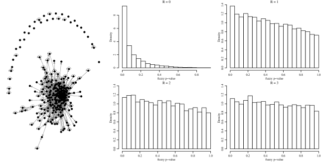
Figure 3: Protein-protein interaction data and histograms of fuzzy $p$-values for models of ranks $R\in\{0,1,2,3\}$. The bins have a width of $0.05$.

As this is a very sparse network (the interaction rate is $\bar{A}=0.03$), we expect a low rank approximation to be appropriate. In fact, analysis using cross validation of a symmetrized version of this data identified $R=3$ to be an appropriate rank in Hoff, (2008). In the right hand side of Figure 3 we present the distributions of the fuzzy $p$-values for $R\in\{0,1,2,3\}$. A visual inspection of the the fuzzy $p$-values in the four panels of the figure provides evidence about the rank of the latent factors. For example, under the $R=0$ model, the $y_{ij}$s are independent and identically distributed, and so the graph represented by the adjacency matrix $A$ is a simple random graph. The fuzzy $p$-values are concentrated at a value lower than 0.05 suggesting a high probability of rejecting the null if $Y$ were observed. For $R\in\{1,2\}$ the fuzzy $p$-values are no longer concentrated lower than 0.05, but the distribution is skewed to the right, which we take as evidence that there is correlation in $Y$ that is not captured by the rank 1 and rank 2 models. The fuzzy $p$-values provide little evidence of residual dependence in $Y$ for models of rank $R\geq 3$.

5 Discussion

In this article we presented a likelihood ratio test for relational datasets. Unlike the previous testing literature for matrix normal models that required multiple observations, and concentrated on testing a null of separable covariances versus an unstructured alternative, we proposed testing a null of no row or column correlations versus an alternative of full row and column correlations using a single observation of a network. While the form of the null distribution of the test statistic is intractable, we are able to simulate a reference distribution for the test statistic under the null due to its invariance to left and right diagonal transformations of the data. In the power simulations of Section 3 we demonstrated the power of the test against maximally sparse and nonseparable alternatives.

This test can be applied to a wide variety of relational data. While the test was developed using the matrix-normal model, we have shown that this distributional assumptions can be greatly relaxed. Specifically, if we consider a data matrix $Y$ with an arbitrary matrix variate elliptically contoured distribution that is centered at the zero matrix, the test statistic for testing for correlation among the rows and among the columns of $Y$ is identical to that of the matrix normal case. We have also demonstrated that the test can accommodate frequently observed features of relational data such as non-zero mean, missing diagonal and multiple observations. In Section 4.2 we demonstrated an application of the theory developed in this paper to binary network data where the matrix $Y$ is an adjacency matrix. The method we describe for binary data can be extended to ordinal and discrete data that can be modeled via a latent matrix variate elliptically contoured distribution.

Once we reject the null hypothesis of independence among the rows and among the columns of a relational matrix, we are faced with the challenge of modeling the dependence in the data. As shown in Section 2.1, for a mean zero matrix normal distribution, the MLE is not unique. Specifically, there is an MLE for each $\Sigma_{\rm r}\in\mathcal{S}^{m}_{+}$ given by $(\Sigma_{\rm r},Y^{t}{\Sigma}_{\rm r}^{-1}Y/m)$. We have observed in separate work that it is possible to distinguish between MLEs by considering their risk. However, other than in very specialized cases (such as equal eigenvalues of $\Sigma_{\rm r}$ and $\Sigma_{\rm c}$), obtaining analytic results for identifying risk optimal MLEs is difficult. The presence of a non-zero mean leads to an unbounded likelihood and further complicates the problem of estimation. Several authors have recently considered Bayesian and penalized likelihood approaches this estimation problem. Bonilla et al., (2008) and Yu et al., (2007) studied hierarchical Gaussian Process priors in the context of a classification problem. In our context, this approach results in a matrix normal prior for the mean parameters and inverse Wishart priors for the row and column covariance matrices. A second approach based on a mixture of independent $L_{1}$ and $L_{2}$ penalties on the row and column precision matrices was proposed by Allen and Tibshirani, (2010).

Computer code and data for the results in Sections 3 and 4 are available at the authors’ websites.

Appendix A Proofs

Proof of Theorem 2.

To show that the solutions to the likelihood equations provide a unique minimizer to the scaled log likelihood function (Equation 1) we will show that the Hessian of $l$ evaluated at the solutions is strictly positive definite and then demonstrate that only a single solution is possible. We rewrite Equation 1 here, explicitly stating that we will be considering diagonal matrices

$$l\left(D_{\rm r},D_{\rm c};Y\right)=-2\log L\left(D_{\rm r},D_{col};Y\right) = {\rm tr}\left[D_{\rm r}^{-1}YD_{\rm c}^{-1}Y^{t}\right]-\log\left|D_{\rm c}^{-1}\otimes D_{\rm r}^{-1}\right|+c,$$

writing for simplicity $\Psi=D_{\rm r}^{-1}$ and $\Gamma=D_{\rm c}^{-1}$ we take first derivatives with respect to the diagonal matrices of $\Gamma$ and $\Psi$:

$$\frac{\partial l\left(D_{\rm r},D_{\rm c};Y\right)}{\partial_{\Psi}} = Y\Gamma Y^{t}\circ I-m\Psi^{-1}$$ (12)

$$\frac{\partial l\left(D_{\rm r},D_{\rm c};Y\right)}{\partial_{\Gamma}} = Y^{t}\Psi Y\circ I-m\Gamma^{-1},$$ (13)

yielding the familiar equations used to find the maximizers of the likelihood. Considering the singular value decomposition of $Y=ALB^{t}$, the above can also be written as partial derivatives with respect to the entries of $\Psi$ and $\Gamma$ (since these are diagonal matrices, the index $k$ refers to the $k^{\rm th}$ row, $k^{\rm th}$ column entry in the matrix):

$$\frac{\partial l\left(D_{\rm r},D_{\rm c};Y\right)}{\partial_{\Psi_{j}}} = \sum_{ikm}L_{i}L_{m}\Gamma_{k}\left(A_{jm}A_{ji}B_{km}B_{ki}\right)-\frac{m}{\Psi_{j}}$$ (14)

$$\frac{\partial l\left(D_{\rm r},D_{\rm c};Y\right)}{\partial_{\Gamma_{k}}} = \sum_{ijm}L_{i}L_{m}\Psi_{j}\left(A_{jm}A_{ji}B_{km}B_{ki}\right)-\frac{m}{\Gamma_{k}}$$ (15)

To compute the Hessian, we take derivatives of equations 14 and 15, yielding the second partial derivatives of $l_{{\rm D}}$:

$$\frac{\partial l\left(D_{\rm r},D_{\rm c};Y\right)}{\partial_{\Psi_{j}\Gamma_{k}}} = f\left(j,k\right)=\sum_{im}L_{i}L_{m}\left(A_{jm}A_{ji}B_{km}B_{ki}\right)=Y_{jk}^{2}$$

$$\frac{\partial l\left(D_{\rm r},D_{\rm c};Y\right)}{\partial_{\Psi_{j}\Psi_{l}}}=\frac{\partial l\left(D_{\rm r},D_{\rm c};Y\right)}{\partial_{\Gamma_{k}\Gamma_{m}}} = 0$$

$$\frac{\partial l\left(D_{\rm r},D_{\rm c};Y\right)}{\partial_{\Psi_{j}\Psi_{j}}} = \frac{m}{\Psi_{j}^{2}}$$

$$\frac{\partial l\left(D_{\rm r},D_{\rm c};Y\right)}{\partial_{\Gamma_{k}\Gamma_{k}}} = \frac{m}{\Gamma_{k}^{2}}.$$

As such, we can write the Hessian matrix $H$ as

$$H = \left[\begin{matrix}m\Psi^{-2}&F\\ F^{t}&m\Gamma^{-2}\end{matrix}\right]$$

where $F=\left[f\left(j,k\right)\right]_{j,k}$. Our first observation is that $F$ is an everywhere positive matrix since $f\left(j,k\right)=Y_{jk}^{2}>0\forall j,k$ (since $P\left(Y\not=0\right)=1$).

To show that $l_{{\rm F}}$ is minimized at the solutions to the likelihood equations 12 and 13 we will show that the Hessian $H$ is strictly positive definite at the solutions. For that, we will verify Sylvester’s criterion: a matrix $H$ is positive definite if and only if all of its leading minors are positive (or equivalently its trailing minors). First we note that the Kronecker product of the covariances leads to a nonidentifiability in the scale of the individual matrices, and so WLOG we let $\Psi_{1}=1$. We consider the reparametrized problem and its’ Hessian $\tilde{H}=H_{-1,-1}$, the Hessian of the original problem with the first row and column removed. Now, the boundedness of the likelihood function implies that the $m-1$ leading minors are positive (since $\hat{\Psi}$ is a positive diagonal matrix) and so we are left with verifying that the remaining $m$ minors are positive. Abusing notation a bit and writing $\Psi$ to correspond to the reparametrized version of row precisions, we get the first minor that includes entries other than those in $\Psi$ is

$$\left|\begin{matrix}m\hat{\Psi}^{-2}&F_{\cdot,1}\\ F_{1,\cdot}&m\hat{\Gamma}_{1}^{-2}\end{matrix}\right| = \left|\frac{m}{\hat{\Gamma}_{1}^{2}}-F_{\cdot,1}\frac{\hat{\Psi}^{2}}{m}F_{1,\cdot}\right|\left|m\hat{\Psi}^{-2}\right|$$

$$:= \left|a\right|\left|b\right|$$

Clearly, $\left|b\right|>0$ as it is simply the previous minor. Now, $a$ does not satisfy the first derivative of $l\left(D_{\rm r},D_{\rm c};Y\right)$ with respect to $\Gamma_{1}$ (Equation 15) and more so we note that

$$\frac{m}{\hat{\Gamma}_{1}^{2}}=\frac{1}{m}\left(\sum_{j}\hat{\Psi}_{j}F_{j,1}\right)^{2}=\frac{1}{m}\left(F_{\cdot,1}\hat{\Psi}^{2}F_{1,\cdot}+c\right)$$

where $c$ is always positive since it is a sum of positive values. Thus, $\left|a\right|=c/m>0$. We can apply this approach to the remaining $m-1$ minors, where the $k$th minor is given by $M_{k}=|a|M_{k-1}$ where $\left|a\right|>0$. Thus we have verified Sylvester’s criterion and have demonstrated that the Hessian of $l\left(D_{\rm r},D_{\rm c};Y\right)$ is strictly positive definite at the solution to the likelihood equations which means we have a local minimum of the scaled log likelihood function (or a local maximum of the likelihood function).

To show uniqueness we apply the Mountain Pass Theorem (page 223 of Courant,, 1950): Since $l\left(D_{\rm r},D_{\rm c};Y\right)$ is smooth, differentiable and coercive (that is $l\left(D_{\rm r},D_{\rm c};Y\right)\rightarrow\infty$ as $\left|D_{\rm c}\otimes D_{\rm r}\right|\rightarrow\infty$), we have that if there are two critical points $x_{1}$ and $x_{2}$ that are strict minima (strictly positive definite Hessian), then there must be another critical point, distinct from $x_{1}$ and $x_{2}$, that is not a relative minimizer of $l$. This contradicts the above notion that the Hessian is strictly positive definite for every critical point. ∎

Proof of Theorem 3.

For $p$ random variables $Y_{1},\dots,Y_{p}$ where $Y_{i}\sim N_{m\times m}\left(0,d_{i}\Sigma_{\rm r},\Sigma_{\rm c}\right)$, we write $D=\left(d_{1},\dots,d_{p}\right)$ and the scaled log likelihood function as

$$l\left(D,\Sigma_{\rm r},\Sigma_{\rm c}|Y_{1},\dots,Y_{p}\right) \propto \sum_{i=1}^{p}\frac{1}{d_{i}}{\rm tr}\left(Y_{i}\Sigma_{\rm c}^{-1}Y_{i}^{t}\Sigma_{\rm r}^{-1}\right)-mp\log\left|\Sigma_{\rm c}^{-1}\right|-mp\log\left|\Sigma_{\rm c}^{-1}\right|-m^{2}\log\left|D^{-1}\right|.$$

Taking first derivatives with respect to $\Sigma_{\rm r}^{-1}$, $\Sigma_{\rm c}^{-1}$ and $d_{i}^{-1}$ and setting them equal to zero yields the likelihood equations:

$$mp\Sigma_{\rm r} = \sum\frac{1}{d_{i}}Y_{i}\Sigma_{\rm c}^{-1}Y_{i}^{t}$$

$$mp\Sigma_{\rm c} = \sum\frac{1}{d_{i}}Y_{i}^{t}\Sigma_{\rm r}^{-1}Y_{i}$$

$$m^{2}d_{i} = {\rm tr}\left(Y_{i}\Sigma_{\rm c}^{-1}Y_{i}^{t}\Sigma_{\rm r}^{-1}\right).$$

We note that when holding $\Sigma_{\rm r}$ and $\Sigma_{\rm c}$ constant, $l\left(D,\Sigma_{\rm r},\Sigma_{\rm c}\right)$ is a strictly convex function of $D^{-1}$ and so with probability 1 it attains a global minimum at points that satisfy the first derivative condition $m^{2}d_{i}={\rm tr}\left(Y_{i}\Sigma_{\rm c}^{-1}Y_{i}^{t}\Sigma_{\rm r}^{-1}\right)$. We define the profile likelihood

$$g\left(\Sigma_{\rm r}^{-1},\Sigma_{\rm c}^{-1}\right) = \inf_{D^{-1}\in\mathbb{R}_{+}^{p}}l\left(D,\Sigma_{\rm r},\Sigma_{\rm c}\right)$$

$$= m^{2}p-mp\log\left|\Sigma_{\rm r}^{-1}\right|-mp\log\left|\Sigma_{\rm c}^{-1}\right|+m^{2}\sum\log\left|{\rm tr}\left(Y_{i}\Sigma_{\rm c}^{-1}Y_{i}^{t}\Sigma_{\rm r}^{-1}\right)\right|+c.$$

There are two nonidentifiabilities in the scaled log likelihood given by $l\left(D,\Sigma_{\rm r},\Sigma_{\rm c}\right)=l\left(aD,b\Sigma_{\rm r},\frac{1}{ab}\Sigma_{\rm c}\right)$ for $a,b>0$ and so we restrict our domain to consider minimization the of $l\left(D,\Sigma_{\rm r},\Sigma_{\rm c}\right)$ over $\mathbb{R}_{+}^{p}\times\mathcal{S}_{2}\times\mathcal{S}_{2}$ where $\mathcal{S}_{2}$ is the bounded subset of $\mathcal{S}_{+}^{m}$ of positive definite matrices whose largest eigenvalue is 1. This makes the model identifiable. Since minimization of $l\left(D,\Sigma_{\rm r},\Sigma_{\rm c}\right)$ is equivalent to minimization of $g\left(\Sigma_{\rm r}^{-1},\Sigma_{\rm c}^{-1}\right)$, we restrict minimizing $g\left(\Sigma_{\rm r}^{-1},\Sigma_{\rm c}^{-1}\right)$ to $\mathcal{S}_{2}\times\mathcal{S}_{2}$. The continuity of $g$ on $\mathcal{S}_{+}^{m}\times\mathcal{S}_{+}^{m}\supset\mathcal{S}_{2}\times\mathcal{S}_{2}$ guarantees that it will attain a minimum on $\mathcal{S}_{2}\times\mathcal{S}_{2}$ as long as for $\overline{\Sigma_{\rm r}^{-1}},\overline{\Sigma_{\rm c}^{-1}}\in\overline{\mathcal{S}_{2}}$

$$\lim_{\Sigma_{\rm r}^{-1}\rightarrow\overline{\Sigma_{\rm r}^{-1}}}g\left(\Sigma_{\rm r}^{-1},\Sigma_{\rm c}^{-1}\right) = g\left(\overline{\Sigma_{\rm r}^{-1}},\Sigma_{\rm c}^{-1}\right)$$

$$\lim_{\Sigma_{\rm c}^{-1}\rightarrow\overline{\Sigma_{\rm c}^{-1}}}g\left(\Sigma_{\rm r}^{-1},\Sigma_{\rm c}^{-1}\right) = g\left(\Sigma_{\rm r}^{-1},\overline{\Sigma_{\rm c}^{-1}}\right)$$

$$\lim_{\Sigma_{\rm c}^{-1}\rightarrow\overline{\Sigma_{\rm c}^{-1}}}\lim_{\Sigma_{\rm r}^{-1}\rightarrow\overline{\Sigma_{\rm r}^{-1}}}g\left(\Sigma_{\rm r}^{-1},\Sigma_{\rm c}^{-1}\right) = g\left(\overline{\Sigma_{\rm r}^{-1}},\overline{\Sigma_{\rm c}^{-1}}\right).$$

All three conditions are met for positive definite boundary points, so all that remains to show is that $g\left(\Sigma_{\rm r}^{-1},\Sigma_{\rm c}^{-1}\right)\rightarrow\infty$ when a subset of the eigenvalues of $\Sigma_{\rm r}^{-1}$ or $\Sigma_{\rm c}^{-1}$ approach 0 (behavior near positive semidefinite boundary points). It is immediate that when the eigenvectors of $\Sigma_{\rm r}^{-1}$ do not match the left eigenvectors of $Y_{i}$ and the eigenvectors of $\Sigma_{\rm c}^{-1}$ do not match the right eigenvectors of $Y_{i}$, ${\rm tr}\left(Y_{i}\Sigma_{\rm c}^{-1}Y_{i}^{t}\Sigma_{\rm r}^{-1}\right)\rightarrow c_{i}>0$, thus the $\log{\rm tr}\left(\cdot\right)$ term converges to a finite constant. As such, the behavior of $g\left(\Sigma_{\rm r}^{-1},\Sigma_{\rm c}^{-1}\right)$ when subsets of eigenvalues approach zero is completely governed by the log determinant terms, both of which will converge to $+\infty$. ∎

References

- Airoldi et al., (2008) Airoldi, E., Blei, D., Fienberg, S., and Xing, E. (2008). Mixed membership stochastic blockmodels. The Journal of Machine Learning Research, 9:1981–2014.
- Allen and Tibshirani, (2010) Allen, G. I. and Tibshirani, R. (2010). Transposable regularized covariance models with an application to missing data imputation. The Annals of Applied Statistics, 4(2):764–790.
- Anderson et al., (1986) Anderson, T., Hsu, H., and Fang, K.-T. (1986). Maximum-likelihood estimates and likelihood-ratio criteria for multivariate elliptically contoured distributions. Canadian Journal of Statistics, 14(1):55–59.
- Bergmann et al., (2003) Bergmann, S., Ihmels, J., and Barkai, N. (2003). Similarities and differences in genome-wide expression data of six organisms. PLoS Biology, 2(1):e9.
- Bergstrand, (1985) Bergstrand, J. (1985). The gravity equation in international trade: some microeconomic foundations and empirical evidence. The review of economics and statistics, pages 474–481.
- Bergstrand, (1989) Bergstrand, J. (1989). The generalized gravity equation, monopolistic competition, and the factor-proportions theory in international trade. The review of economics and statistics, pages 143–153.
- Bonilla et al., (2008) Bonilla, E., Chai, K. M., and Williams, C. (2008). Multi-task gaussian process prediction.
- Butland et al., (2005) Butland, G., Peregrín-Alvarez, J. M., Li, J., Yang, W., Yang, X., Canadien, V., Starostine, A., Richards, D., Beattie, B., Krogan, N., et al. (2005). Interaction network containing conserved and essential protein complexes in escherichia coli. Nature, 433(7025):531–537.
- Courant, (1950) Courant, R. (1950). Dirichlet’s principle, conformal mapping, and minimal surfaces. Interscience Publishers, Inc, New York.
- Dawid, (1981) Dawid, A. (1981). Some matrix-variate distribution theory: notational considerations and a bayesian application. Biometrika, 68(1):265–274.
- Eaton, (1983) Eaton, M. (1983). Multivariate statistics: a vector space approach. Wiley New York.
- Eriksen, (1987) Eriksen, P. S. (1987). Proportionality of covariance matrices. Ann. Statist., 15(2):732–748.
- Fletcher et al., (2011) Fletcher, A., Bonell, C., and Sorhaindo, A. (2011). You are what your friends eat: systematic review of social network analyses of young people’s eating behaviours and bodyweight. Journal of epidemiology and community health, 65(6):548–555.
- Flury, (1986) Flury, B. K. (1986). Proportionality of k covariance matrices. Statistics & probability letters, 4(1):29–33.
- Gupta and Varga, (1994) Gupta, A. and Varga, T. (1994). A new class of matrix variate elliptically contoured distributions. Statistical Methods & Applications, 3(2):255–270.
- Gupta and Varga, (1995) Gupta, A. and Varga, T. (1995). Some inference problems for matrix variate elliptically contoured distributions. Statistics: A Journal of Theoretical and Applied Statistics,, 26(3):219–229.
- Hoff, (2005) Hoff, P. (2005). Bilinear mixed-effects models for dyadic data. J. Amer. Statist. Assoc., 100(469):286–295.
- Hoff, (2008) Hoff, P. (2008). Modeling homophily and stochastic equivalence in symmetric relational data. In Platt, J., Koller, D., Singer, Y., and Roweis, S., editors, Advances in Neural Information Processing Systems 20, pages 657–664. MIT Press, Cambridge, MA.
- Hoff, (2011) Hoff, P. (2011). Separable covariance arrays via the tucker product, with applications to multivariate relational data. Bayesian Analysis, 6(2):179–196.
- Hoff et al., (2002) Hoff, P., Raftery, A., and Handcock, M. (2002). Latent space approaches to social network analysis. Journal of the american Statistical association, 97(460):1090–1098.
- Holland et al., (1983) Holland, P., Laskey, K., and Leinhardt, S. (1983). Stochastic blockmodels: first steps. Social networks, 5(2):109–137.
- Jensen and Johansen, (1987) Jensen, S. T. and Johansen, S. (1987). Estimation of proportional covariances. Statistics & probability letters, 6(2):83–85.
- Jensen and Madsen, (2004) Jensen, S. T. and Madsen, J. (2004). Estimation of proportional covariances in the presene of certain linear restrictions. The Annals of Statistics, 32(1):219–232.
- Kenny and La Voie, (1984) Kenny, D. and La Voie, L. (1984). The social relations model. Advances in experimental social psychology, 18:142–182.
- Lafosse and Ten Berge, (2006) Lafosse, R. and Ten Berge, J. (2006). A simultaneous concor algorithm for the analysis of two partitioned matrices. Computational statistics & data analysis, 50(10):2529–2535.
- Lazzarini et al., (2001) Lazzarini, S., Chaddad, F., and Cook, M. (2001). Integrating supply chain and network analyses: the study of netchains. Journal on chain and network science, 1(1):7–22.
- Leskovec et al., (2008) Leskovec, J., Lang, K., Dasgupta, A., and Mahoney, M. (2008). Statistical properties of community structure in large social and information networks. In Proceeding of the 17th international conference on World Wide Web, pages 695–704. ACM.
- Li, (2006) Li, H. (2006). The covariance structure and likelihood function for multivariate dyadic data. J. Multivariate Anal., 97(6):1263–1271.
- Li and Loken, (2002) Li, H. and Loken, E. (2002). A unified theory of statistical analysis and inference for variance component models for dyadic data. Statist. Sinica, 12(2):519–535.
- Lincoln and Gerlach, (2004) Lincoln, J. and Gerlach, M. (2004). Japan’s network economy: structure, persistence, and change. Cambridge University Press.
- Lu and Zimmerman, (2005) Lu, N. and Zimmerman, D. (2005). The likelihood ratio test for a separable covariance matrix. Statistics & probability letters, 73(4):449–457.
- McQuitty and Clark, (1968) McQuitty, L. and Clark, J. (1968). Clusters from iterative, intercolumnar correlational analysis. Educational and psychological measurement.
- Mitchell et al., (2006) Mitchell, M., Genton, M., and Gumpertz, M. (2006). A likelihood ratio test for separability of covariances. Journal of Multivariate Analysis, 97(5):1025–1043.
- Nowicki and Snijders, (2001) Nowicki, K. and Snijders, T. (2001). Estimation and prediction for stochastic blockstructures. Journal of the American Statistical Association, 96(455):1077–1087.
- Panning, (1982) Panning, W. (1982). Fitting blockmodels to data. Social Networks, 4(1):81–101.
- Pollard et al., (2010) Pollard, M., Tucker, J., Green, H., Kennedy, D., and Go, M. (2010). Friendship networks and trajectories of adolescent tobacco use. Addictive behaviors, 35(7):678–685.
- Potter et al., (2012) Potter, G., Handcock, M., Longini, I., and Halloran, M. (2012). Estimating within-school contact networks to understand influenza transmission. Ann. Appl. Stat., 6(1):1–26.
- Rohe et al., (2011) Rohe, K., Chatterjee, S., and Yu, B. (2011). Spectral clustering and the high-dimensional stochastic blockmodel. The Annals of Statistics, 39(4):1878–1915.
- Roy and Khattree, (2005) Roy, A. and Khattree, R. (2005). On implementation of a test for kronecker product covariance structure for multivariate repeated measures data. Statistical Methodology, 2(4):297–306.
- Sampson, (1968) Sampson, S. (1968). A novitiate in a period of change: An experimental and case study of social relationships. PhD thesis, Cornell University, September.
- Srivastava et al., (2008) Srivastava, M., von Rosen, T., and Von Rosen, D. (2008). Models with a kronecker product covariance structure: estimation and testing. Mathematical Methods of Statistics, 17(4):357–370.
- Stuart et al., (2003) Stuart, J., Segal, E., Koller, D., and Kim, S. (2003). A gene-coexpression network for global discovery of conserved genetic modules. Science, 302(5643):249–255.
- Thompson and Geyer, (2007) Thompson, E. and Geyer, C. (2007). Fuzzy p-values in latent variable problems. Biometrika, 94(1):49–60.
- Tinbergen et al., (1962) Tinbergen, J. et al. (1962). Shaping the world economy: Suggestions for an international economic policy. Twentieth Century Fund New York.
- Tseng, (2001) Tseng, P. (2001). Convergence of a block coordinate descent method for nondifferentiable minimization. Journal of optimization theory and applications, 109(3):475–494.
- Van De Bunt et al., (1999) Van De Bunt, G., Van Duijn, M., and Snijders, T. (1999). Friendship networks through time: An actor-oriented dynamic statistical network model. Computational & Mathematical Organization Theory, 5(2):167–192.
- Wang and Wong, (1987) Wang, Y. and Wong, G. (1987). Stochastic blockmodels for directed graphs. Journal of the American Statistical Association, 82(397):8–19.
- (48) Westveld, A. and Hoff, P. (2011a). A mixed effects model for longitudinal relational and network data, with applications to international trade and conflict. Ann. Appl. Stat., 5(2A):843–872.
- (49) Westveld, A. H. and Hoff, P. D. (2011b). A mixed effects model for longitudinal relational and network data, with applications to international trade and conflict. Ann. Appl. Stat., 5(2A):843–872.
- White et al., (1976) White, H., Boorman, S., and Breiger, R. (1976). Social structure from multiple networks. i. blockmodels of roles and positions. American journal of sociology, pages 730–780.
- Yu et al., (2007) Yu, K., Chu, W., Yu, S., Tresp, V., and Xu, Z. (2007). Stochastic relational models for discriminative link prediction. Advances in neural information processing systems, 19:1553.