Linear multi-step schemes for BSDEs

Abstract

We study the convergence rate of a class of linear multi-step methods for BSDEs. We show that, under a sufficient condition on the coefficients, the schemes enjoy a fundamental stability property. Coupling this result to an analysis of the truncation error allows us to design approximation with arbitrary order of convergence. Contrary to the analysis performed in [22], we consider general diffusion model and BSDEs with driver depending on $z$. The class of methods we consider contains well known methods from the ODE framework as Nystrom, Milne or Adams methods. We also study a class of Predictor-Correctot methods based on Adams methods. Finally, we provide a numerical illustration of the convergence of some methods.

Key words: Backward SDEs, High order discretization, Linear multi-step methods.

MSC Classification (2000): 60H10, 65C30.

1 Introduction

In this paper, we are interested in the discrete-time approximation of solutions of (decoupled) Backward Stochastic Differential Equation (BSDE), i.e. a triplet $(X,Y,Z)$ satisfying

$$X_{t} =X_{0}+\int_{0}^{t}b(X_{s})\mathrm{d}s+\int_{0}^{t}\sigma(X_{s})\mathrm{d}W_{s},$$ (1.1)

$$Y_{t} =g(X_{T})+\int_{t}^{T}f(Y_{t},Z_{t})\mathrm{d}t-\int_{t}^{T}Z_{t}\mathrm{d}W_{t}\,.$$ (1.2)

The function $(b,\sigma):\mathbb{R}^{d}\mapsto\mathbb{R}^{d}\times{\cal M}_{d}$, and $f:\mathbb{R}\times\mathbb{R}^{d}\mapsto\mathbb{R}$ are Lipschitz-continuous function, $g:\mathbb{R}^{d}\mapsto\mathbb{R}$ is differentiable with continuous and bounded first derivative. The positive constant $T$ is given and $W$ is a Brownian motion supported by a filtered probability space $(\Omega,{\cal F},({\cal F})_{0\leq t\leq T},\mathbb{P})$. The process $Y$ is a one-dimensional stochastic process, the processes $X$ and $Z$ are valued in $\mathbb{R}^{d}$ and $Z$ is written, by convention, as a row vector. Under the Lipschitz assumption on the coefficients, the processes $X$ and $Y$ belong to the set ${\cal S}^{2}$ of continuous adapted processes with square integrable supremum and $Z$ belongs to ${\cal H}^{2}$, the set of progressively measurable processes satisfying $\mathbb{E}\!\!\left[\int_{0}^{T}|Z_{s}|^{2}\mathrm{d}s\right]$.

The existence and uniqueness of solutions of the system (1.1) -(1.2) was first addressed by Pardoux and Peng in [16]. Moreover, in [17], they show that

$$Y_{t}=u(t,X_{t}),\ \ \ \ Z_{t}=\nabla u^{\!\top}\!(t,X_{t})\sigma(X_{t}),\ \ \ \ t\in[0,T],$$

where $u\in C^{1,2}([0,T]\times\mathbb{R}^{d})$ is the solution of the final value Cauchy problem

$$L^{(0)}u(t,x) =-f\left(u(t,x),\nabla u^{\!\top}\!(t,x)\sigma\left(x\right)\right),\quad t\in[0,T),\,x\in\mathbb{R}^{d}$$ (1.3)

$$u(T,x) =g(x),\quad x\in\mathbb{R}^{d}$$ (1.4)

with $L^{(0)}$ defined to be the second order differential operator

$$L^{(0)}=\partial_{t}+\sum_{i=1}^{d}b_{i}\partial_{x_{i}}+\frac{1}{2}\sum_{i,j=1}^{d}a_{ij}\partial_{x_{i}}\partial_{x_{j}},$$ (1.5)

and $a=a_{ij}=\sigma\sigma^{\top}$.

To approximate (1.1)-(1.2), one has to come up with an approximation of the SDE part and the BSDE part. Obtaining approximations of the distribution of the forward component $X$ has been largely resolved in the last thirty years. There is a large literature on the subject and one can refer to [15] and the references therein for a systematic study of numerical methods for approximating $X$.

Here, we focus on the approximation of $(Y,Z)$ instead. Numerical methods approximating this backward component have already been proposed. They are mainly based on a Euler approximation, see [3, 23, 13, 8] and the references therein. These methods have been successfully extended to a broader class of BSDEs: reflected BSDEs [1, 6], BSDEs with jumps [2], BSDEs with driver of quadratic growth [18], see also the reference therein. In a very specific framework, [20, 19, 21, 22] proposed some high order methods to approximate the solution of the BSDE. Recently high order method of Runge-Kutta type have been studied [9, 7] in the general framework of (1.1)-(1.2).

In this paper, we consider another type of high order method, very well known for ODEs, namely linear multi-step methods.

The approximations presented below are associated to an arbitrary, but fixed, partition $\pi$ of the interval $[0,T]$, $\pi=\{t_{0}=0<\dots<t_{i}<t_{i+1}<\dots<t_{n}=T\}$. We define $h_{i}=t_{i+1}-t_{i}$, $i=0,...,n-1$ and $|\pi|=\max_{i}h_{i}$ and denote by $(Y_{i},Z_{i})$ the approximation of $(Y_{t_{i}},Z_{t_{i}})$ for $i=1,...,n$. The construction of the approximating process is done in a recursive manner, backwards in time. We describe in the following the salient features of the class of approximations considered in this paper.

Definition 1.1.

(Linear multi-step methods)

(i) To initialise the scheme with $r$ steps, $r\geq 1$, we are given $r$ terminal condition $(Y_{n-j},Z_{n-j})$, ${\cal F}_{t_{n-j}}$-measurable square integrable random variables, $0\leq j\leq r-1$.

(ii) For $i\leq n-r$, the computation of $(Y_{i},Z_{i})$ involves $r$ steps and is given by

$$\left\{\begin{array}[]{rcl}Y_{i}&=&\mathbb{E}_{t_{i}}\!\!\left[\sum_{j=1}^{r}a_{j}Y_{i+j}+h\sum_{j=0}^{r}b_{i,j}f(Y_{i+j},Z_{i+j})\right]\vspace{2mm}\\ Z_{i}&=&\mathbb{E}_{t_{i}}\!\!\left[\sum_{j=1}^{r}\alpha_{j}H^{Y}_{i,j}Y_{i+j}+h\sum_{j=1}^{r}\beta_{i,j}H^{f}_{i,j}f(Y_{i+j},Z_{i+j})\right]\end{array}\right.$$

where $a_{j}$, $b_{i,j}$, $\alpha_{j}$, $\beta_{i,j}$ are real numbers satisfying

$$|a_{j}|+|b_{i,j}|+|\alpha_{j}|+|\beta_{i,j}|\leq\Lambda\;,\;0\leq i\leq n-r\;,0\leq j\leq r\;,$$

and $\Lambda$ is a positive constant. We impose the so-called pre-consistency condition i.e.

$$\sum_{j=1}^{r}{a_{j}}=\sum_{j=1}^{r}{\alpha_{j}}=1\;.$$

The coefficients $H^{Y}_{i,j}$, $H^{f}_{i,j}$, $0\leq i\leq n-r$, $1\leq j\leq r$ are ${\cal F}_{t_{i+j}}$-measurable random variables satisfying, for all $j$,

$$h_{i}\mathbb{E}\!\!\left[|H^{Y}_{i,j}|^{2}+|H^{f}_{i,j}|^{2}\right]\leq\Lambda\quad\text{ and }\quad\mathbb{E}_{t_{i}}\!\!\left[H^{Y}_{i,j}\right]=\mathbb{E}_{t_{i}}\!\!\left[H^{f}_{i,j}\right]=0\,.$$

Remark 1.1.

(i) The value $(Y_{n},Z_{n})$ is generally given by $(g(X_{T}),\nabla g^{\top}(X_{T})\sigma(X_{T}))$. If $r>1$, one needs to specify other initialisation values. This choice is important because it will impact the global rate of convergence. One can use Runge-Kutta type scheme [7] with high order of convergence.

(ii) When $r=1$, schemes 1.1 are one-step scheme. See [3, 23, 13, 9, 7] and the references therein for a study of these schemes.

The global error we investigate here is a time discretization error and is, given a grid $\pi$, $({\cal E}_{Y}(\pi),{\cal E}_{Z}(\pi))$ with

$${\cal E}_{Y}(\pi):=\max_{i}\mathbb{E}\!\!\left[|Y_{t_{i}}-Y_{i}|^{2}\right]\text{ and }{\cal E}_{Z}(\pi):=\sum_{i}h_{i}\mathbb{E}\!\!\left[|Z_{t_{i}}-Z_{i}|^{2}\right].$$

To implement high order scheme in practice, we need to specify a particular form for the $H$-coefficient appearing in Definition 1.1 above. Let us first introduce a special class of random variables, which was already considered in [7].

Definition 1.2.

(i) For $m\geq 0$, we denote by ${\cal B}^{m}_{[0,1]}$ the set of bounded measurable function $\psi:[0,1]\rightarrow\mathbb{R}$ satisfying

$$\int_{0}^{1}\psi(u)\mathrm{d}u=1\text{ and if }m\geq 1,\;\int_{0}^{1}\psi(u)u^{k}\mathrm{d}u=0\;,\;1\leq k\leq m.$$

(ii) Let $(\psi^{\ell})_{1\leq\ell\leq d}\in{\cal B}^{m}_{[0,1]}$, for $t\in[0,T]$ and $h>0$ s.t. $t+h\leq T$, we define,

$$H^{\psi}_{t,h}:=(\frac{1}{h}\int_{t}^{t+h}\psi^{\ell}(\frac{u-t}{h})\mathrm{d}W^{\ell}_{u})_{1\leq\ell\leq d}\;,$$

which is a row vector.

By convention, we set $H^{\psi}_{t,0}=0$.

In the sequel, when studying the order of convergence of the scheme and depending of the order we want to retrieve, we will assume that, for $1\leq j\leq r$,

$$H^{Y}_{i,j}:=H^{\psi}_{t_{i},jh}\text{ and }H^{f}_{i,j}:=H^{\phi}_{t_{i},jh}$$ (1.6)

for some functions $\psi$ and $\phi$ in ${\cal B}^{m}$, $m\geq 0$, see Theorem 2.1 below.

The convergence analysis is done in a classical way. We first prove a fundamental stability property for the schemes, under a reasonable sufficient condition, see Proposition 2.1. Then, assuming smoothness of the value function $u$ given by (1.3)-(1.4), we study the truncation error associated to the above methods. We prove a sufficient condition on the coefficient to retrieve methods of any order. These two steps allow us to retrieve general convergence and design new high order method for BSDEs. Contrary to the analysis performed in [22], we work with general diffusion model given by (1.1) and BSDEs with driver depending on $z$. As an example of application, we extend some classical scheme used in the ODE framework and then proceed with the study of Adams type methods. Based on these methods, we also design Predictor-Corrector methods and study their convergence. To the best of our knowledge, it is the first time that these methods are considered for BSDEs. Finally, we illustrate our theoretical results with some numerical experiments showing empirical convergence rates.

The rest of this paper is organised as follows. In section 2, we prove our general convergence result which relies heavily on a stability property. In section 3, we study Adams methods and Predictor-Corrector methods in the context of BSDEs. The main results are stated in the multi-dimensional case but for the reader’s convenience the proofs are done with $d=1$. Finally, in section 4, we provide a numerical example.

Notations

We denote by $\mathcal{M}_{d}$ the set of matrices with $d$ lines and $d$ columns. For a matrix $A\in{\cal M}_{d}$, $\text{Tr}[A]$ denotes its trace, $A^{.j}$ its $j$-th column, $A^{i.}$ its $i$-th row, and $A^{ij}$ the $i$-th term of $A^{.j}$. $I_{d}$ is the identity matrix of ${\cal M}_{d}$. The transpose of a matrix or a vector $y$ will be denoted $y^{\top}$. The sup-norm for both vectors and matrix is denoted $|\,.\,|_{\infty}$.

In the sequel $C$ is a positive constant whose value may change from line to line depending on $T$, $d$, $\Lambda$, $X_{0}$ but which does not depend on $\pi$. We write $C_{p}$ if it depends on some positive parameters $p$.

For $t\in\pi$, $R$ a random variable and $r$ a real number, the notation $R=O_{t}(r)$ means that $|U|\leq\lambda^{\pi}_{t}u$ where $\lambda^{\pi}_{t}$ is a positive random variable satisfying:

$$\mathbb{E}\!\!\left[|\lambda^{\pi}_{t}|^{p}\right]\leq C_{p}\;,$$

for all $p>0$, $t\in\pi$ and all grid $\pi$.

2 General convergence results

In this part, we study the convergence properties of the schemes given in Definition 1.1.

We first establish a stability property for the schemes. We then state a sufficient condition on the coefficients which allows us to retrieve high order schemes.

2.1 $L^{2}$-stability

To investigate the stability of the schemes given in Definition 1.1, we introduce a pertubed scheme

$$\left\{\begin{array}[]{rcl}\tilde{Y}_{i}&=&\mathbb{E}_{t_{i}}\!\!\left[\sum_{j=1}^{r}a_{j}\tilde{Y}_{i+j}+h\sum_{j=0}^{r}b_{i,j}f(\tilde{Y}_{i+j},\tilde{Z}_{i+j})\right]+\zeta^{Y}_{i}\vspace{1mm}\\ \tilde{Z}_{i}&=&\mathbb{E}_{t_{i}}\!\!\left[\sum_{j=1}^{r}\alpha_{j}H^{Y}_{i,j}\tilde{Y}_{i+j}+h\sum_{j=1}^{r}\beta_{i,j}H^{f}_{i,j}f(\tilde{Y}_{i+j},\tilde{Z}_{i+j})\right]+\zeta^{Z}_{i}\end{array}\right.$$ (2.3)

where $\zeta^{Y}_{i}$, $\zeta^{Z}_{i}$ are random variables belonging to $L^{2}({\cal F}_{t_{i}})$, for $i\leq n-r$.

The notion of stablity we consider here is the following.

Definition 2.1.

($L^{2}$-Stability) The scheme given in Definition 1.1 is said to be $L^{2}$-stable if

$$\max_{0\leq i\leq n-r}\mathbb{E}\!\!\left[|\delta Y_{i}|^{2}\right] +\sum_{i=0}^{n-r}h_{i}\mathbb{E}\!\!\left[|\delta Z_{i}|^{2}\right]\leq$$

$$C\Big{(}\max_{0\leq j\leq r-1}\mathbb{E}\!\!\left[|\delta Y_{n-j}|^{2}+|\pi||\delta Z_{n-j}|^{2}\right]+|\pi|\sum_{i=0}^{n-r}\mathbb{E}\!\!\left[\frac{1}{h_{i}^{2}}|{\zeta^{Y}_{i}}|^{2}+|{\zeta^{Z}_{i}}|^{2}\right]\Big{)}$$

for all sequences $\zeta^{Y}_{i}$,$\zeta^{Z}_{i}$ of $L^{2}({\cal F}_{t_{i}})$-random variable, $i\leq n-r$, and terminal values $(Y_{n-j},Z_{n-j})$, $(\tilde{Y}_{n-j},\tilde{Z}_{n-j})$ belonging to $L^{2}({\cal F}_{t_{n-j}})$, $0\leq j\leq r-1$.

Proposition 2.1.

Assume that the following holds

• The coefficients $(a_{j})$ are non-negative, $\sum_{j=1}^{r}a_{j}=1$ and for $1\leq j\leq r$, $a_{j}=0\implies\alpha_{j}=0$,

then, the scheme given in Definition 1.1 is $L^{2}$-stable, recalling Definition 2.1.

Proof.

We define $U_{i}=(Y_{i},\dots,Y_{i+r-1})^{\top}$, $\tilde{U}_{i}=(\tilde{Y}_{i},\dots,\tilde{Y}_{i+r-1})^{\top}$, and

$$\Phi^{Y}_{i} =\left(\begin{array}[]{c}\sum_{j=0}^{r}b_{i,j}f(Y_{i+j},Z_{i+j})\\ \mathbf{0}\\ \end{array}\right)_{r,1}\text{ , }\tilde{\Phi}^{Y}_{i}=\left(\begin{array}[]{c}\sum_{j=0}^{r}b_{i,j}f(\tilde{Y}_{i+j},\tilde{Z}_{i+j})\\ \mathbf{0}\\ \end{array}\right)_{r,1}$$

and $$\tilde{\Theta}^{Y}_{i}=\left(\begin{array}[]{c}\zeta^{Y}_{i}\\ \mathbf{0}\\ \end{array}\right)_{r,1}$$

and denote $\delta U_{i}=U_{i}-\tilde{U}_{i}$, $\delta\Phi^{Y}_{i}=\Phi^{Y}_{i}-\tilde{\Phi}^{Y}_{i}$,

$$a=(a_{1},\dots,a_{r}),\;\alpha=(\alpha_{1},\dots,\alpha_{r})\text{ and }A=\left(\begin{array}[]{c|c}a_{1},\dots,a_{r-1}&a_{r}\\ \hline\cr I_{r-1}&\mathbf{0}\\ \end{array}\right)_{r,r}\;.$$

The scheme and the pertubed scheme rewrite then for the $Y$ part

$$\mathbb{E}_{t_{i}}\!\!\left[U_{i}\right] =\mathbb{E}_{t_{i}}\!\!\left[AU_{i+1}+h\Phi^{Y}_{i}\right]$$

and

$$\mathbb{E}_{t_{i}}\!\!\left[\tilde{U}_{i}\right] =\mathbb{E}_{t_{i}}\!\!\left[A\tilde{U}_{i+1}+h\tilde{\Phi}^{Y}_{i}+\Theta^{Y}_{i}\right]\;.$$

1.a

For $i\leq j\leq n-r$, we compute that

$$|\mathbb{E}_{t_{i}}\!\!\left[\delta U_{j}\right]|_{\infty}\leq|A|_{\infty}|\mathbb{E}_{t_{i}}\!\!\left[\delta U_{j+1}\right]|_{\infty}+h_{j}|\mathbb{E}_{t_{i}}\!\!\left[\delta\Phi^{Y}_{j}\right]|_{\infty}+|\mathbb{E}_{t_{i}}\!\!\left[\Theta^{Y}_{j}\right]|_{\infty}$$

Under $({\mathbb{H}c})$, we observe that $|A|_{\infty}=1$ and we get

$$|\mathbb{E}_{t_{i}}\!\!\left[\delta U_{j}\right]|_{\infty}\leq|\mathbb{E}_{t_{i}}\!\!\left[\delta U_{j+1}\right]|_{\infty}+h_{j}|\mathbb{E}_{t_{i}}\!\!\left[\delta\Phi^{Y}_{j}\right]|_{\infty}+|\mathbb{E}_{t_{i}}\!\!\left[\Theta^{Y}_{j}\right]|_{\infty}$$

Iterating on $j$, we compute that

$$|\mathbb{E}_{t_{i}}\!\!\left[\delta U_{j}\right]|_{\infty}\leq|\mathbb{E}_{t_{i}}\!\!\left[\delta U_{n-r+1}\right]|_{\infty}+\sum_{k=j}^{n-r}h_{k}|\mathbb{E}_{t_{i}}\!\!\left[\delta\Phi^{Y}_{k}\right]|_{\infty}+\sum_{k=j}^{n-r}|\mathbb{E}_{t_{i}}\!\!\left[\Theta^{Y}_{k}\right]|_{\infty}\;.$$

In particular, we have for $i=j$, and $|\pi|$ small enough,

$$|\delta Y_{i}|\leq C\Big{(}\sum_{k=i}^{n-r}h_{k}\mathbb{E}_{t_{i}}\!\!\left[|\delta Y_{k}|+|\delta Z_{k}|\right]+\sum_{k=i}^{n-r}\mathbb{E}_{t_{i}}\!\!\left[|\zeta^{Y}_{k}|\right]+\sum_{k=n-r+1}^{n}\mathbb{E}_{t_{i}}\!\!\left[|\delta Y_{k}|\right]\Big{)}\;.$$ (2.4)

We then compute

$$\mathbb{E}\!\!\left[|\delta Y_{i}|^{2}\right]\leq C\Big{(}|\pi|\sum_{k=i}^{n-r}\mathbb{E}\!\!\left[|\delta Y_{k}|^{2}\right]+\sum_{k=i}^{n-r}h_{k}\mathbb{E}\!\!\left[|\delta Z_{k}|^{2}\right] +\sum_{k=i}^{n-r}\frac{1}{h_{k}}\mathbb{E}\!\!\left[|\zeta^{Y}_{k}|^{2}\right]+\sum_{k=n-r+1}^{n}\mathbb{E}\!\!\left[|\delta Y_{k}|^{2}\right]\Big{)}\;.$$ (2.5)

1.b We will now control the term $h\sum_{k=i}^{n-r}\mathbb{E}\!\!\left[|\delta Z_{k}|^{2}\right]$ appearing in (2.5).

Using Cauchy-Schwartz inequality, we obtain that, if $a_{j}\neq 0$ then

$$|\mathbb{E}_{t_{i}}\!\!\left[\alpha_{j}H_{i,j}^{Y}\delta Y_{i+j}\right]|^{2} \leq C(a_{j}\mathbb{E}_{t_{i}}\!\!\left[|\delta Y_{i+j}|^{2}-a_{j}|\mathbb{E}_{t_{i}}\!\!\left[\delta Y_{i+j}\right]|^{2}\right])$$

which leads to, under $({\mathbb{H}c})$,

$$h_{i}\mathbb{E}\!\!\left[|\delta Z_{i}|^{2}\right] \leq C\Big{(}\sum_{j=1}^{r}a_{j}\mathbb{E}\!\!\left[|\delta Y_{i+j}|^{2}\right]-\sum_{j=1}^{r}\mathbb{E}\!\!\left[a_{j}|\mathbb{E}_{t_{i}}\!\!\left[\delta Y_{i+j}\right]|^{2}\right])$$

$$\quad+|\pi|^{2}\sum_{j=1}^{r}\mathbb{E}\!\!\left[|\delta Y_{i+j}|^{2}+|\delta Z_{i+j}|^{2}\right]+|\pi|\mathbb{E}\!\!\left[|\zeta^{Z}_{i}|^{2}\right]\;.\Big{)}$$ (2.6)

Under $({\mathbb{H}c})$, we have that,

$$-\sum_{j=1}^{r}\mathbb{E}\!\!\left[a_{j}|\mathbb{E}_{t_{i}}\!\!\left[\delta Y_{i+j}\right]|^{2}\right] \leq-\mathbb{E}\!\!\left[|\sum_{j=1}^{r}\mathbb{E}_{t_{i}}\!\!\left[a_{j}\delta Y_{i+j}\right]|^{2}\right]\;.$$

Then, recalling that

$$\sum_{j=1}^{r}\mathbb{E}_{t_{i}}\!\!\left[a_{j}\delta Y_{i+j}\right]=\delta Y_{i}-h_{i}\sum_{j=0}^{r}\mathbb{E}_{t_{i}}\!\!\left[\delta\Phi^{Y}_{j+r}\right]-\zeta^{Y}_{i}$$

we compute

$$-\sum_{j=1}^{r}\mathbb{E}\!\!\left[|\mathbb{E}_{t_{i}}\!\!\left[a_{j}\delta Y_{i+j}\right]|^{2}\right] \leq-\mathbb{E}\!\!\left[|\delta Y_{i}|^{2}\right]+C|\pi|\mathbb{E}\!\!\left[|\delta Y_{i}|\sum_{j=0}^{r}\mathbb{E}_{t_{i}}\!\!\left[|\delta Y_{i+j}|+|\delta Z_{i+j}|\right]\right]+C\mathbb{E}\!\!\left[|\delta Y_{i}|\,|\zeta^{Y}_{i}|\right]$$

which leads, for $0<\epsilon\leq 1$ to be fixed later on, to

$$-\sum_{j=1}^{r}\mathbb{E}\!\!\left[|\mathbb{E}_{t_{i}}\!\!\left[a_{j}\delta Y_{i+j}\right]|^{2}\right] \leq-\mathbb{E}\!\!\left[|\delta Y_{i}|^{2}\right]+C|\pi|\sum_{j=0}^{r}\mathbb{E}_{t_{i}}\!\!\left[\frac{1}{\epsilon}|\delta Y_{i+j}|^{2}+\epsilon|\delta Z_{i+j}|^{2}\right]+\frac{C}{h_{i}}\mathbb{E}\!\!\left[|\zeta^{Y}_{i}|^{2}\right]\;.$$

Combining the last inequality with (2.1) and summing over $i$, we obtain, for $|\pi|$ small enough

$$\sum_{k=i}^{n-r}h_{k}\mathbb{E}\!\!\left[|\delta Z_{k}|^{2}\right] \leq C\Big{(}\sum_{k=i}^{n-r}(\sum_{j=1}^{r}a_{j}\mathbb{E}\!\!\left[|\delta Y_{i+j}|^{2}\right]-\mathbb{E}\!\!\left[|\delta Y_{i}|^{2}\right])+C(1+\frac{1}{\epsilon})|\pi|\sum_{k=n-r+1}^{n}\mathbb{E}\!\!\left[|\delta Y_{k}|^{2}+|\delta Z_{k}|^{2}\right]$$

$$+C(1+\frac{1}{\epsilon})|\pi|\sum_{k=i}^{n-r}\mathbb{E}\!\!\left[|\delta Y_{k}|^{2}\right]+\frac{C}{\epsilon}|\pi|\sum_{k=i}^{n-r}\mathbb{E}\!\!\left[|\delta Z_{k}|^{2}\right]+|\pi|\sum_{k=i}^{n-r}\mathbb{E}\!\!\left[|{\zeta^{Z}_{k}}|^{2}\right]+\sum_{k=i}^{n-r}\frac{C}{h_{k}}\mathbb{E}\!\!\left[|{\zeta^{Y}_{k}}|^{2}\right]\Big{)}$$

Using $({\mathbb{H}c})$, setting $\epsilon:=\frac{C}{2}$, we then obtain

$$\sum_{k=i}^{n-r}h_{k}\mathbb{E}\!\!\left[|\delta Z_{k}|^{2}\right] \leq C\Big{(}\sum_{k=n-r+1}^{n}\mathbb{E}\!\!\left[|\delta Y_{k}|^{2}+|\pi||\delta Z_{k}|^{2}\right]+|\pi|\sum_{k=i}^{n-r}\mathbb{E}\!\!\left[|\delta Y_{k}|^{2}\right]+\sum_{k=i}^{n-r}\mathbb{E}\!\!\left[\frac{1}{h_{k}}|{\zeta^{Y}_{k}}|^{2}+h_{k}|{\zeta^{Z}_{k}}|^{2}\right]\Big{)}$$ (2.7)

1.c Combining the last inequality with (2.5), we get

$$\mathbb{E}\!\!\left[|\delta Y_{i}|^{2}\right]\leq C\Big{(}|\pi|\sum_{j=i}^{n-r}\mathbb{E}\!\!\left[|\delta Y_{j}|^{2}\right]+\sum_{k=i}^{n-r}|\pi|\mathbb{E}\!\!\left[\frac{1}{h_{k}^{2}}|\mathbb{E}_{t_{k}}\!\!\left[\zeta^{Y}_{k}\right]|^{2}+|\mathbb{E}_{t_{k}}\!\!\left[\zeta^{Z}_{k}\right]|^{2}\right]+\sum_{k=n-r+1}^{n}\mathbb{E}\!\!\left[|\delta Y_{k}|^{2}+|\pi||\delta Z_{k}|^{2}\right]\Big{)}$$ (2.8)

2.a Let us define

$$\delta_{i} :=\sum_{j=i}^{n-r}\mathbb{E}\!\!\left[|\delta Y_{j}|^{2}\right]\;,$$

$$\theta_{i} :=\sum_{k=i}^{n-r}|\pi|\mathbb{E}\!\!\left[\frac{1}{h_{k}^{2}}|{\zeta^{Y}_{k}}|^{2}+|{\zeta^{Z}_{k}}|^{2}\right]+\sum_{k=n-r+1}^{n}\mathbb{E}\!\!\left[|\delta Y_{k}|^{2}+|\pi||\delta Z_{k}|^{2}\right]\;.$$

Equation (2.8) reads then

$$\delta_{i}-\delta_{i+1}\leq C|\pi|\delta_{i}+C\theta_{i}$$ (2.9)

Using a discrete version of Gronwall Lemma, we then compute

$$\delta_{i}\leq C(\delta_{n-r}+\sum_{k=i}^{n-r}\theta_{k}e^{C(n-r-k)|\pi|})$$

Since $\delta_{n-r}\leq\eta_{i}$ and $\theta_{k}\leq\theta_{i}$ for $k\geq i$, we compute

$$\delta_{i}\leq C\theta_{i}\frac{1}{1-e^{C|\pi|}}$$

This last equation combined with (2.9) leads to

$$\mathbb{E}\!\!\left[|\delta Y_{i}|^{2}\right]\leq C\theta_{i}$$

which concludes the proof for the $Y$-part.

2.b For the $Z$-part, the proof is concluded pluging last inequality in (2.7), with $i=0$ in this equation. $\Box$

Remark 2.1.

It is easily checked that $({\mathbb{H}c})$ implies that the roots of the following polynomial equations

$$y^{r+1}-\sum_{j=1}^{r}a_{j}y^{r-j+1}=0\,.$$

are in the closed unit disc and the multiple roots are in the open unit disc.
It is known that in the ODEs framework this is a necessary and sufficient condition to get stability of linear multi-step schemes, see e.g [5, 11]. In our context, this condition is only necessary. We have to imposed $({\mathbb{H}c})$ essentially because we need to deal with the new process $Z$.

Remark 2.2.

Proposition 2.1 is generic in the sense that we do not use the particular property of the probability space nor the fact that $({\cal F}_{t})_{t\in[0,T]}$ is a Brownian filtration. We will use this property in the last section of this paper.

2.2 Study of the order

2.2.1 Definitions

To study the order of the schemes, we use the following definition of truncation errors.

The local truncation error for the pair $(Y,Z)$ defined as

$$\eta_{i}:=\eta^{Y}_{i}+\eta^{Z}_{i},\ \ \ \ (\eta^{Y}_{i},\eta^{Z}_{i}):=\left(\frac{1}{h_{i}^{2}}\mathbb{E}\!\!\left[|Y_{t_{i}}-\check{Y}_{t_{i}}|^{2}\right],\mathbb{E}\!\!\left[|Z_{t_{i}}-\check{Z}_{t_{i}}|^{2}\right]\right),\;i\leq n-r\;,$$ (2.10)

with

$$\check{Y}_{t_{i}} =\mathbb{E}_{t_{i}}\!\!\left[\sum_{j=1}^{r}a_{j}Y_{t_{i+j}}+h_{i}\sum_{j=1}^{r}b_{i,j}f(Y_{t_{i+j}},Z_{t_{i+j}})+h_{i}b_{i,0}f(\check{Y}_{t_{i}},\check{Z}_{t_{i}})\right]$$ (2.11)

$$\check{Z}_{t_{i}} =\mathbb{E}_{t_{i}}\!\!\left[\sum_{j=1}^{r}\alpha_{j}H^{\psi}_{t_{i},jh}Y_{t_{i+j}}+h_{j}\sum_{j=1}^{r}\beta_{i,j}H^{\phi}_{t_{i},jh}f(Y_{t_{i+j}},Z_{t_{i+j}})\right]$$ (2.12)

where $\psi$, $\phi$ belongs to ${\cal B}^{0}$.

The global truncation error for a given grid $\pi$ is given by

$${\cal T}(\pi):={\cal T}_{Y}(\pi)+\mathcal{T}_{Z}(\pi),\ \ \ ({\cal T}_{Y}(\pi),{\cal T}_{Z}(\pi)):=\left(\sum_{i=0}^{n-r}h_{i}\eta^{Y}_{i},\ \ \ \sum_{i=0}^{n-r}h_{i}\eta^{Z}_{i}\right),$$ (2.13)

where ${\cal T}_{Y}$ is the global truncation error for $Y$ and ${\cal T}_{Z}$ is the global truncation error for $Z$ defined as above.

Definition 2.2.

An approximation is said to have a global truncation error of order $m$ if we have

$${\cal T}(\pi)\leq C|\pi|^{2m}$$

for all sufficiently smooth solutions to (1.3) and all partitions $\pi$ with sufficiently small mesh size.

2.2.2 Expansion of the truncation error

We study the order of the methods given in Definition 1.1 using Itô-Taylor expansions [15]. This requires the smoothness of the value function $u$ introduced in (1.3)-(1.4). In order to state precisely these assumptions, we recall some notations of Chapter 5 (see Section 5.4) in [15].

Let

$${\cal M}:=\{\oslash\}\cup\bigcup_{m=1}^{\infty}\{0,\dots,d\}^{m}$$

be the set of multi-indices with entries in $\{0,\dots,d\}$ endowed with the measure $\ell$ of the length of a multi-index ($\ell(\oslash)=0$ by convention).

We introduce the concatenation operator $*$ on ${\cal M}$ for multi-indices with finite length: $\alpha=(\alpha_{1},\dots,\alpha_{p})$, $\beta=(\beta_{1},\dots,\beta_{q})$ then $\alpha*\beta=(\alpha_{1},\dots,\alpha_{p},\beta_{1},\dots,\beta_{q})$.

A non empty subset ${\cal A}\subset{\cal M}$ is called a hierarchical set if

$$\sup_{\alpha}\ell(\alpha)<\infty\text{ and }-\alpha\in{\cal A},\;\forall\alpha\in{\cal A}\setminus\{\oslash\}$$

For any hierarchical ${\cal A}$ set, we consider the remainder set ${\cal B}({\cal A})$ given by

$${\cal B}({\cal A}):=\{\alpha\in{\cal M}\setminus{\cal A}|-\alpha\in{\cal A}\}$$

We will use in the sequel the following sets of multi-indices, for $n\geq 0$:

$${\cal A}_{n}:=\{\alpha\;|\;\ell(\alpha)\leq n\}$$

and observe that ${\cal B}({\cal A}_{n})={\cal A}_{n+1}\setminus{\cal A}_{n}$.

For $j\in\{1,\dots,d\}$, we consider the operators:

$$L^{(j)}=\sum_{k=1}^{d}\sigma^{kj}\partial_{x_{k}}.$$

For a multi-index $\alpha=(\alpha_{1},\dots,\alpha_{p})$, the iteration of these operators has to be understood in the following sense

$$L^{\alpha}:=L^{(\alpha_{1})}\circ\dots\circ L^{(\alpha_{p})}.$$

By convention, $L^{\oslash}$ is the identity operator, recall also the definition of $L^{(0)}$ given in (1.5). One can observe that $L^{\alpha*\beta}=L^{\alpha}\circ L^{\beta}$.

For a multi-index with finite length $\alpha$, we consider the set ${\cal G}^{\alpha}$ of function $v:[0,T]\times\mathbb{R}^{d}\rightarrow\mathbb{R}$ for which $L^{\alpha}v$ is well defined and continuous. We also introduce ${\cal G}^{\alpha}_{b}$ the subset of function $v\in{\cal G}^{\alpha}$ such that the function $L^{\alpha}v$ is bounded. For $v\in{\cal G}^{\alpha}$, we denote $L^{\alpha}u$ by $u^{\alpha}$.

Finally, for $n\geq 1$, we define the set ${\cal G}^{n}_{b}$ of function $u$ such that $u^{\alpha}\in{\cal G}^{\alpha}_{b}$ for all $\alpha\in{\cal A}_{n}\setminus\{\oslash\}$.

The two following Propositions are key results to prove the high order rate of convergence of the schemes. We refer to [7] for proofs.

Proposition 2.2.

Assume $d=1$. Let $m\geq 0$, then for a function $v\in{\cal G}^{m+1}_{b}$, we have that

$$\mathbb{E}_{t}\!\!\left[v(t+h,X_{t+h})\right] =v_{t}+hv_{t}^{(0)}+\frac{h^{2}}{2}v_{t}^{(0,0)}+\dots+\frac{h^{m}}{m!}v_{t}^{(0)_{m}}+O_{t}(h^{m+1})$$

Proposition 2.3.

Assume $d=1$. (i) Let $m\geq 0$, for $\psi\in{\cal B}^{m}_{[0,1]}$, assuming that $v\in{\cal G}^{m+2}_{b}$, we have

$$\mathbb{E}_{t}\!\!\left[H^{\psi}_{t,h}v(t+h,X_{t+h})\right] =v^{(1)}_{t}+hv^{(1,0)}_{t}+\dots+\frac{h^{m}}{m!}v^{(1)*(0)_{m}}_{t}+O_{t}(h^{m+1})$$

(ii) For $\psi\in{\cal B}^{0}_{[0,1]}$, assuming that $v\in{\cal G}^{1}_{b}$, we have

$$\mathbb{E}_{t}\!\!\left[H^{\psi}_{t,h}v(t+h,X_{t+h})\right] =O_{t}(1)\,.$$

(iii) If $L^{(0)}\circ L^{(1)}=L^{(1)}\circ L^{(0)}$, then the expansion of (i) holds true with $\psi=1$.

2.2.3 Sufficient condition for Order $m$

For the reader’s convenience, we assume in this paragraph a constant time step for the grid $\pi$ i.e. $h_{i}=h=|\pi|:=\frac{T}{n}$, for all $i$ and that the coefficients $b$, $\beta$ do not depend of $i$.

Under these conditions, the scheme given in Definition 1.1, recalling (1.6), rewrites, for $i\leq n-r$,

$$\left\{\begin{array}[]{rcl}Y_{i}&=&\mathbb{E}_{t_{i}}\!\!\left[\sum_{j=1}^{r}a_{j}Y_{i+j}+h\sum_{j=0}^{r}b_{j}f(Y_{i+j},Z_{i+j})\right]\vspace{2mm}\\ Z_{i}&=&\mathbb{E}_{t_{i}}\!\!\left[\sum_{j=1}^{r}\alpha_{j}H^{\psi}_{t_{i},jh}Y_{i+j}+h\sum_{j=1}^{r}\beta_{j}H^{\phi}_{t_{i},jh}f(Y_{i+j},Z_{i+j})\right]\end{array}\right.$$ (2.16)

Proposition 2.4.

(Order m) For $m\geq 2$, assume that the following holds

$$(C^{Y})_{m} :\;\;\sum_{j=1}^{r}a_{j}j^{p}-p\sum_{j=0}^{r}b_{j}j^{p-1}=0,\;1\leq p\leq m$$

$$\text{ and }\quad(C^{Z})_{m} :\;\;\sum_{j=1}^{r}\alpha_{j}j^{p}-p\beta_{j}j^{p-1}=0,\;1\leq p\leq m-1$$

and that $u\in{\cal G}^{m+1}_{b}$, then we have

$${\cal T}_{Y}(\pi)+{\cal T}_{Z}(\pi)\leq C|\pi|^{2m},$$

provided that $\psi\in{\cal B}^{m-1}_{[0,1]}$ and $\phi\in{\cal B}^{m-2}_{[0,1]}$, recalling (2.16).

Proof.

1. We first study the truncation error for the Z-part. We have that

$$\check{Z}_{t_{i}} =\mathbb{E}_{t_{i}}\!\!\left[\sum_{j=1}^{r}\alpha_{j}H^{\psi}_{t_{i},jh}Y_{t_{i+j}}+h\sum_{j=1}^{r}\beta_{j}H^{\phi}_{t_{i},jh}f(Y_{t_{i+j}},Z_{t_{i+j}})\right]$$

$$=\mathbb{E}_{t_{i}}\!\!\left[\sum_{j=1}^{r}\alpha_{j}H^{\psi}_{t_{i},jh}u(t_{i+j},X_{t_{i+j}})-h\sum_{j=1}^{r}\beta_{j}H^{\phi}_{t_{i},jh}u^{(0)}(t_{i+j},X_{t_{i+j}})\right]\;.$$

Using Proposition 2.3, we compute

$$\check{Z}_{t_{i}}=\sum_{p=0}^{m-1}\sum_{j=1}^{r}\alpha_{j}j^{p}\frac{h^{p}}{p!}u^{(1)*(0)_{p}}(t_{i},X_{t_{i}})-\sum_{p=0}^{m-2}\sum_{j=1}^{r}\beta_{j}j^{p}\frac{h^{p+1}}{p!}u^{(1)*(0)_{p+1}}(t_{i},X_{t_{i}})+O_{t_{i}}(|\pi|^{m})$$

which leads to

$$\check{Z}_{t_{i}} -Z_{t_{i}}=(\sum_{j=1}^{r}\alpha_{j}-1)u^{(1)}(t_{i},X_{t_{i}})+\sum_{p=1}^{m-1}\frac{h^{p}}{p!}u^{(1)*(0)_{p}}(t_{i},X_{t_{i}})(\sum_{j=1}^{r}\alpha_{j}j^{p}-p\sum_{j=1}^{r}j^{p-1}\beta_{j})+O_{t_{i}}(|\pi|^{m})$$

Under $(C^{Z})_{m}$, we obtain

$$\check{Z}_{t_{i}} -Z_{t_{i}}=O_{t_{i}}(|\pi|^{m})$$

which leads directly to

$$\eta^{Z}_{i}=O(|\pi|^{2m}),\quad i\leq n-r.$$ (2.17)

2.a We now study the truncation error for the Y-part. Let us introduce

$$\bar{Y}_{t_{i}} =\mathbb{E}_{t_{i}}\!\!\left[\sum_{j=1}^{r}a_{j}Y_{t_{i+j}}+h\sum_{j=0}^{r}b_{j}f(Y_{t_{i+j}},Z_{t_{i+j}})\right]$$

We have that

$$\check{Y}_{t_{i}} =\bar{Y}_{t_{i}}+hb_{0}\Big{(}f(\check{Y}_{t_{i}},\check{Z}_{t_{i}})-f(Y_{t_{i}},Z_{t_{i}})\Big{)}$$

Since $f$ is Lipschitz-continuous, we get that for $|\pi|$ small enough,

$$\check{Y}_{t_{i}}-Y_{t_{i}}=O_{t_{i}}(\bar{Y}_{t_{i}}-Y_{t_{i}})+|\pi|O_{t_{i}}(\check{Z}_{t_{i}}-Z_{t_{i}})\;.$$ (2.18)

2.b Now observe that

$$\bar{Y}_{t_{i}} =\mathbb{E}_{t_{i}}\!\!\left[\sum_{j=1}^{r}a_{j}u(t_{i+j},X_{t_{i+j}})-h\sum_{j=0}^{r}b_{j}u^{(0)}(t_{i+j},X_{t_{i+j}})\right]\;.$$

Using Proposition 2.2, we compute

$$\bar{Y}_{t_{i}}=\sum_{p=0}^{m}\sum_{j=1}^{r}a_{j}j^{p}\frac{h^{p}}{p!}u^{(0)_{p}}(t_{i},X_{t_{i}})-\sum_{p=0}^{m-1}\sum_{j=0}^{r}b_{j}j^{p}\frac{h^{p+1}}{p!}u^{(0)_{p+1}}(t_{i},X_{t_{i}})+O_{t_{i}}(|\pi|^{m+1})$$

which leads to

$$\bar{Y}_{t_{i}} -Y_{t_{i}}=(\sum_{j=1}^{r}a_{j}-1)u(t_{i},X_{t_{i}})+\sum_{p=1}^{m}\frac{h^{p}}{p!}u^{(0)_{p}}(t_{i},X_{t_{i}})(\sum_{j=1}^{r}a_{j}j^{p}-p\sum_{j=0}^{r}j^{p-1}b_{j})+O_{t_{i}}(|\pi|^{m+1}).$$

Under $(C^{Y})_{m}$, we thus get

$$\bar{Y}_{t_{i}} -Y_{t_{i}}=O_{t_{i}}(|\pi|^{m+1})$$

2.c Combining the last inequality with (2.18) and (2.17), we then obtain

$$\eta^{Y}_{i}=O(|\pi|^{2m+2})\;,\;i\leq n-r\;.$$

3. Combining the last equation with (2.17), we conclude that

$${\cal T}(\pi)=O(|\pi|^{2m}),$$

and so the scheme is of order $m$.

$\Box$

2.3 Convergence results and examples of high order methods

Theorem 2.1.

Under $({\mathbb{H}c})$, assuming that the scheme is of order $m$ according to Definition 2.2 and that

$$\max_{0\leq j\leq r-1}\mathbb{E}\!\!\left[|Y_{t_{n-j}}-Y_{n-j}|^{2}+h|Z_{t_{n-j}}-Z_{n-j}|^{2}\right]\leq C|\pi|^{2m}$$ (2.19)

we have

$${\cal E}_{Y}(\pi)+{\cal E}_{Z}(\pi)\leq C|\pi|^{2m}\;.$$

Proof. We simply observe that the solution $(Y,Z)$ of the BSDE is also the solution of a perturbed scheme with $\zeta^{Y}_{i}:=\check{Y}_{t_{i}}-Y_{t_{i}}$ and $\zeta^{Z}_{i}:=\check{Z}_{t_{i}}-Z_{t_{i}}$. The proof then follows directly from Proposition 2.1. $\Box$

In particular, in the special setting of paragraph 2.2.3, a straightforward application of Theorem 2.1 and Proposition 2.4 leads to

Corollary 2.1.

Under $({\mathbb{H}c})$ and $(C^{Y})_{m}$- $(C^{Z})_{m}$, assuming that (2.19) holds, we have

$${\cal E}_{Y}(\pi)+{\cal E}_{Z}(\pi)\leq C|\pi|^{2m}\;,$$

provided $u\in{\cal G}^{m+1}_{b}$ and $\psi\in{\cal B}^{m-1}_{[0,1]}$, $\phi\in{\cal B}^{m-2}_{[0,1]}$.

To illustrate the previous results, we conclude this section by giving two examples of high order method which can be designed using Corollary 2.1.

Example 2.1.

(Nystrom’s method) The following scheme is –for the Y-part– inspired by the Leap-frog (or Nystrom’s) method for ODE, namely

$$\left\{\begin{array}[]{rcl}Y_{i}&=&\mathbb{E}_{t_{i}}\!\!\left[Y_{i+2}+2hf(Y_{i+1},Z_{i+1})\right]\vspace{2mm}\\ Z_{i}&=&\mathbb{E}_{t_{i}}\!\!\left[H^{\psi}_{t_{i},2h}Y_{i+2}+2hH^{\phi}_{t_{i},2h}f(Y_{i+2},Z_{i+2})\right].\end{array}\right.$$

This 2-step method is convergent and the rate of convergence is at least of order 2, assuming that $u\in{\cal G}^{3}_{b}$ and $\psi\in{\cal B}^{1}_{[0,1]}$, $\phi\in{\cal B}^{0}_{[0,1]}$.

Example 2.2.

(Milne’s method) The second scheme we propose is inspired –for the Y-part– by the Milne’s method for ODE, namely

$$\left\{\begin{array}[]{rcl}Y_{i}&=&\mathbb{E}_{t_{i}}\!\!\left[Y_{i+4}+h\Big{(}\frac{8}{3}f(Y_{i+1},Z_{i+1})-\frac{4}{3}f(Y_{i+2},Z_{i+2})+\frac{8}{3}f(Y_{i+3},Z_{i+3})\Big{)}\right]\vspace{2mm}\\ Z_{i}&=&\mathbb{E}_{t_{i}}\!\!\left[H^{\psi}_{t_{i},4h}Y_{i+4}+h\Big{(}\frac{8}{3}H^{\phi}_{t_{i},h}f(Y_{i+1},Z_{i+1})-\frac{4}{3}H^{\phi}_{t_{i},2h}f(Y_{i+2},Z_{i+2})+\frac{8}{3}H^{\phi}_{t_{i},3h}f(Y_{i+3},Z_{i+3})\Big{)}\right].\end{array}\right.$$

This 4-step method is convergent and the rate of convergence is at least of order 4, assuming that $u\in{\cal G}^{5}_{b}$ and $\psi\in{\cal B}^{3}_{[0,1]}$, $\phi\in{\cal B}^{2}_{[0,1]}$.

3 Adams Methods

In this section, we introduce methods for BSDEs inspired by Adams methods from the ODE framework. These methods are of two kinds: explicit methods , also called Adams-Bashforth, or implicit methods, also called, Adams-Moulton.

The schemes introduced in Definition 1.1 are always explicit for the $Z$-part but may be implicit for the $Y$-part. So, for the $Z$-part, we use Adams-Bashforth approximation which may then be combined with explicit or implicit approximation for the $Y$-part.

We first study methods combining Adams-Moulton type approximation for the $Y$-part and Adams-Bashforth type approximation for the $Z$-part. We show that these methods are really efficient because high order rate of convergence can be achieved, assuming smoothness of the value function. We then quickly discuss the case of explicit methods, i.e. Adams-Bashforth type approximation both for the $Y$-part and $Z$-part.

At the end of this section, we use these Adams type approximation to design Predictor-Corrector methods for BSDEs.

3.1 Implicit methods

These methods are inspired by Adams-Moulton method for the $Y$-part and Adams-Bashforth for the $Z$-part.

They have the following form, for $i\leq n-r$,

$$(AMB)_{r}\,:\;\left\{\begin{array}[]{rcl}Y_{i}&=&\mathbb{E}_{t_{i}}\!\!\left[Y_{i+1}+h_{i}\sum_{j=0}^{r}b_{i,j,r}f(Y_{i+j},Z_{i+j})\right]\vspace{2mm}\\ Z_{i}&=&\mathbb{E}_{t_{i}}\!\!\left[H^{\psi}_{t_{i},h}Y_{i+1}+h_{i}\sum_{j=1}^{r}\beta_{i,j,r}H^{\phi}_{t_{i},jh}f(Y_{i+j},Z_{i+j})\right]\end{array}\right.$$

where $\psi,\phi\in{\cal B}^{0}_{[0,1]}$.

The coefficients for the $Y$-part are given by

$$b_{i,j,r}=\frac{1}{h_{i}}\int_{t_{i}}^{t_{i+1}}L_{i,j,r}(s)\mathrm{d}s\,,\;\text{ with }L_{i,j,r}(t)=\displaystyle\prod_{k=0,k\neq j}^{r}\frac{t-t_{i+k}}{t_{i+j}-t_{i+k}}\;,\;0\leq j\leq r.$$ (3.1)

The Lagrange polynomials $L_{i,j,r}$ are of degree $r$ and $L_{i,j,r}(t_{i+j})=1$, which implies

$$\sum_{j=0}^{r}(t_{i+j}-t_{i})^{k}L_{i,j,r}(t)=(t-t_{i})^{k}\,,\quad 0\leq k\leq r\,.$$ (3.2)

The definition of the $b$-coefficients means that

$$Y_{i}=\mathbb{E}_{t_{i}}\!\!\left[Y_{i+1}+\int_{t_{i}}^{t_{i+1}}Q^{Y}_{i,r}(t)\mathrm{d}t\right]$$

where $Q^{Y}_{i,r}$ is a polynomial of degree less than $r$ satisfying

$$Q^{Y}_{i,r}(t_{i+j})=f(Y_{i+j},Z_{i+j})\;,\;0\leq j\leq r\;.$$

In the case where the time step is constant, the coefficient does not depends on $i$ and are given by

$$b_{j,r}=\int_{0}^{1}\ell_{j,r}(s)\mathrm{d}s\,,\;\text{ with }\ell_{j,r}(s)=\displaystyle\prod_{k=0,k\neq j}^{r+1}\frac{s-k}{j+1-k}\;,\;0\leq j\leq r\;.$$

The coefficients for the $Z$-part are given by

$$\beta_{i,j,r}=\frac{1}{h_{i}}\int_{t_{i}}^{t_{i+1}}\tilde{L}_{i,j,r}(s)\mathrm{d}s\,,\;1\leq j\leq r,\text{ with }\tilde{L}_{i,j,r}(s)=\displaystyle\prod_{k=1,k\neq j}^{r}\frac{t-t_{i+k}}{t_{i+j}-t_{i+k}}\;.$$ (3.3)

The Lagrange polynomials $\tilde{L}_{i,j,r}$ are of degree $r-1$ and $\tilde{L}_{i,j,r}(t_{i+j})=1$, which implies

$$\sum_{j=1}^{r}(t_{i+j}-t_{i})^{k}\tilde{L}_{i,j,r}(t)=(t-t_{i})^{k}\,,\quad 0\leq k\leq r-1\,.$$ (3.4)

The definition of the $\beta$-coefficients means that

$$Z_{i}=\mathbb{E}_{t_{i}}\!\!\left[H^{\psi}_{t_{i},h}Y_{i+1}+\int_{t_{i}}^{t_{i+1}}Q^{Z}_{i,r}(t)\mathrm{d}t\right]$$

where $Q^{Z}_{i,r}$ is a polynomial of degree less than $r-1$ satisfying

$$Q^{Z}_{i,r}(t_{i+j})=H^{\phi}_{t_{i},jh}f(Y_{i+j},Z_{i+j})\;,\;1\leq j\leq r\;.$$

In the case where the time step is constant, the coefficient does not depends on $i$ and are given by

$$\beta_{j,r}=\int_{0}^{1}\ell_{j,r}(s)\mathrm{d}s\,,\;\text{ with }\ell_{j,r}(s)=\displaystyle\prod_{k=1,k\neq j}^{r}\frac{s-k}{j-k}\;.$$

When the time step is constant, the table below gives the $b$-coefficients and $\beta$-coefficients for $r\leq 4$:

$$\begin{array}[]{c|ccccc|cccc}r&b_{0}&b_{1}&b_{2}&b_{3}&b_{4}&\beta_{1}&\beta_{2}&\beta_{3}&\beta_{4}\\ \hline\cr 1&\frac{1}{2}&\frac{1}{2}&&&&1&&&\\ 2&\frac{5}{2}&\frac{8}{12}&-\frac{1}{12}&&&\frac{3}{2}&-\frac{1}{2}&&\\ 3&\frac{9}{24}&\frac{19}{24}&-\frac{5}{24}&\frac{1}{24}&&\frac{23}{12}&-\frac{16}{12}&\frac{5}{12}&\\ 4&\frac{251}{720}&\frac{646}{720}&-\frac{264}{720}&\frac{106}{720}&-\frac{19}{720}&\frac{55}{24}&-\frac{59}{24}&\frac{37}{24}&-\frac{9}{24}\end{array}$$

Proposition 3.1.

The $(AMB)_{r}$ method is convergent and at least of order $r+1$, provided that $\psi\in{\cal B}^{r}$, $\phi\in{\cal B}^{r-1}$ and $u\in{\cal G}^{r+2}_{b}$.

Proof. 1. The stability of the schemes comes from a direct application of Proposition 2.1, since obviously $({\mathbb{H}c})$ holds for $(AMB)_{r}$. Following Theorem 2.1, we only have to study the order of the method.

2.a We first study the error for the $Z$ part. Observe that, recalling (2.12),

$$\check{Z}_{t_{i}} :=\mathbb{E}_{t_{i}}\!\!\left[H^{\psi}_{t_{i},h}Y_{t_{i+1}}+\sum_{j=1}^{r}H^{\phi}_{t_{i},jh}f(Y_{t_{i+j}},Z_{t_{i+j}})\int_{t_{i}}^{t_{i+1}}L_{i,j,r}(t)\mathrm{d}t\right]$$

$$=\mathbb{E}_{t_{i}}\!\!\left[H^{\psi}_{t_{i},h}u(t_{i+1},X_{t_{i+1}})-\sum_{j=1}^{r}H^{\phi}_{t_{i},jh}u^{(0)}(t_{i+j},X_{t_{i+j}})\int_{t_{i}}^{t_{i+1}}L_{i,j,r}(t)\mathrm{d}t\right]$$

Using Proposition 2.3, we get

$$\check{Z}_{t_{i}}-Z_{t_{i}}=\sum_{k=1}^{r}\frac{h_{i}^{k}}{k!}u^{(1)*(0)_{k}}(t_{i},X_{t_{i}})-\sum_{j=1}^{r}\int_{t_{i}}^{t_{i+1}}\tilde{L}_{i,j,r}(t)\mathrm{d}t\sum_{k=0}^{r-1}\frac{u^{(1)*(0)_{k+1}}(t_{i},X_{t_{i}})}{k!}(t_{i+j}-t_{i})^{k}+O_{t_{i}}(|\pi|^{r+1})$$

which reads also

$$\check{Z}_{t_{i}}-Z_{t_{i}}=\sum_{k=1}^{r}\frac{h_{i}^{k}}{k!}u^{(1)*(0)_{k}}(t_{i},X_{t_{i}})-\sum_{k=0}^{r-1}\frac{u^{(1)*(0)_{k+1}}(t_{i},X_{t_{i}})}{k!}\int_{t_{i}}^{t_{i+1}}\sum_{j=1}^{r}(t_{i+j}-t_{i})^{k}\tilde{L}_{i,j,r}(t)\mathrm{d}t+O_{t_{i}}(|\pi|^{r+1})\;.$$

Using (3.4), we obtain

$$\check{Z}_{t_{i}}-Z_{t_{i}} =\sum_{k=1}^{r}\Big{(}\frac{h_{i}^{k}}{k!}-\frac{1}{(k-1)!}\int_{t_{i}}^{t_{i+1}}(t-t_{i})^{k-1}\mathrm{d}t\Big{)}u^{(1)*(0)_{k}}(t_{i},X_{t_{i}})+O_{t_{i}}(|\pi|^{r+1})$$

$$=O_{t_{i}}(|\pi|^{r+1}).$$

2.b We now study the truncation error for the $Y$ part. Let us define,

$$\bar{Y}_{t_{i}} :=\mathbb{E}_{t_{i}}\!\!\left[Y_{t_{i+1}}+\sum_{j=0}^{r}f(Y_{t_{i+j}},Z_{t_{i+j}})\int_{t_{i}}^{t_{i+1}}L_{i,j,r}(t)\mathrm{d}t\right]$$

Observe that

$$\check{Y}_{t_{i}} :=\bar{Y}_{t_{i}}+\Big{(}f(\check{Y}_{t_{i}},\check{Z}_{t_{i}})-f(Y_{t_{i}},Z_{t_{i}})\Big{)}\int_{t_{i}}^{t_{i+1}}L_{i,0,r}(t)\mathrm{d}t$$

which leads since $f$ is Lipschitz continuous, for $|\pi|$ small enough, to

$$\check{Y}_{t_{i}}-Y_{t_{i}}=O_{t_{i}}(|\bar{Y}_{t_{i}}-Y_{t_{i}}|)+|\pi|O_{t_{i}}(|\check{Z}_{t_{i}}-Z_{t_{i}}|)\;.$$ (3.5)

Now,

$$\bar{Y}_{t_{i}} =\mathbb{E}_{t_{i}}\!\!\left[u(t_{i+1},X_{t_{i+1}})-\sum_{j=0}^{r}u^{(0)}(t_{i+1},X_{t_{i+1}})\int_{t_{i}}^{t_{i+1}}L_{i,j,r}(t)\mathrm{d}t\right]$$

Using Proposition 2.2, we get

$$\bar{Y}_{t_{i}}-Y_{t_{i}}=\sum_{k=1}^{r+1}\frac{h_{i}^{k}}{k!}u^{(0)_{k}}(t_{i},X_{t_{i}})-\sum_{j=0}^{r}\int_{t_{i}}^{t_{i+1}}L_{i,j,r}(t)\mathrm{d}t\sum_{k=0}^{r}\frac{u^{(0)_{k+1}}(t_{i},X_{t_{i}})}{k!}(t_{i+j}-t_{i})^{k}+O_{t_{i}}(|\pi|^{r+2})$$

which reads also

$$\bar{Y}_{t_{i}}-Y_{t_{i}}=\sum_{k=1}^{r+1}\frac{h_{i}^{k}}{k!}u^{(0)_{k}}(t_{i},X_{t_{i}})-\sum_{k=0}^{r}\frac{u^{(0)_{k+1}}(t_{i},X_{t_{i}})}{k!}\int_{t_{i}}^{t_{i+1}}\sum_{j=0}^{r}(t_{i+j}-t_{i})^{k}L_{i,j,r}(t)\mathrm{d}t+O_{t_{i}}(|\pi|^{r+2})\;.$$

Using (3.2), we obtain

$$\bar{Y}_{t_{i}}-Y_{t_{i}} =\sum_{k=1}^{r+1}\Big{(}\frac{h_{i}^{k}}{k!}-\frac{1}{(k-1)!}\int_{t_{i}}^{t_{i+1}}(t-t_{i})^{k-1}\mathrm{d}t\Big{)}u^{(0)_{k}}(t_{i},X_{t_{i}})+O_{t_{i}}(|\pi|^{r+2})$$

$$=O_{t_{i}}(|\pi|^{r+2}).$$

Thus, using (3.5),

$$\check{Y}_{t_{i}}-Y_{t_{i}}=O_{t_{i}}(|\pi|^{r+2}).$$

2.c Combining the results of steps 1.a and 1.b, we obtain

$${\cal T}(\pi)=O_{t_{i}}(|\pi|^{r+1})\;.$$

which concludes the proof. $\Box$

3.2 Explicit methods

These methods are inspired by Adams-Bashforth method both for the $Y$-part and $Z$-part.

$$(ABB)_{r}\left\{\begin{array}[]{rcl}Y_{i}&=&\mathbb{E}_{t_{i}}\!\!\left[Y_{i+1}+h_{i}\sum_{j=1}^{r}b_{i,j,r}f(Y_{i+j},Z_{i+j})\right]\vspace{2mm}\\ Z_{i}&=&\mathbb{E}_{t_{i}}\!\!\left[H^{\psi}_{t_{i},h}Y_{i+1}+h_{i}\sum_{j=1}^{r}\beta_{i,j,r}H^{\phi}_{t_{i},jh}f(Y_{i+j},Z_{i+j})\right]\end{array}\right.$$

where $\psi,\phi\in{\cal B}^{0}_{[0,1]}$.

Now, the coefficients for the $Y$-part are given by

$$b_{i,j,r}=\frac{1}{h_{i}}\int_{t_{i}}^{t_{i+1}}\tilde{L}_{i,j,r}(s)\mathrm{d}s\,,$$

recalling (3.3).

From the proof of Proposition 3.1, step 1.b. we know that we can obtain a truncation error for the $Z$-part s.t. $\hat{Z_{t_{i}}}-Z_{t_{i}}=O_{t_{i}}(|\pi|^{r+1})$. But here, due to the explicit feature of the $Y$ part and thus an order $r$ global error only, we only need to retrieve an error for the $Z$-part of order $r$ as well. This simply means that the scheme, for the $Z$-part, has one more coefficient than needed. So one can set

$$\beta_{i,j,r}=b_{i,j,r}$$

or

$$\beta_{i,r,r}=0\text{ and }\beta_{i,j,r}=b_{i,j,r-1},\;1\leq j\leq r-1\;.$$

Following the arguments of the proof of Proposition 3.1, one obtains

Proposition 3.2.

The $(ABB)_{r}$ method is convergent and at least of order $r$, provided that $\psi\in{\cal B}^{r-1}$, $\phi\in{\cal B}^{r-2}$ and $u\in{\cal G}^{r+1}_{b}$.

3.3 Predictor-Corrector methods

These methods are fully explicit method but have a better rate of convergence than the $(ABB)_{r}$ methods presented above. Nevertheless, they require the computation of one more conditional expectation by step. This has to be compared in practice to the Picard Iteration required by $(AMB)_{r}$ approximation.

Definition 3.1.

$$(PC)_{r}\left\{\begin{array}[]{rcl}Z_{i}&=&\mathbb{E}_{t_{i}}\!\!\left[H^{\psi}_{t_{i},h}Y_{i+1}+h_{i}\sum_{j=1}^{r}\beta_{i,j,r}H^{\phi}_{t_{i},jh}f(Y_{i+j},Z_{i+j})\right]\vspace{2mm}\\ {}^{p}Y_{i}&=&\mathbb{E}_{t_{i}}\!\!\left[Y_{i+1}+h_{i}\sum_{j=1}^{r}\beta_{i,j,r}f(Y_{i+j},Z_{i+j})\right]\vspace{2mm}\\ Y_{i}&=&\mathbb{E}_{t_{i}}\!\!\left[Y_{i+1}+h_{i}\sum_{j=1}^{r}b_{i,j,r}f(Y_{i+j},Z_{i+j})\right]+h_{i}b_{i,0,r}f({}^{p}Y_{i},Z_{i})\end{array}\right.$$ (3.9)

where $\psi,\phi\in{\cal B}^{0}_{[0,1]}$. The $b$-coefficients are given by (3.1) and the $\beta$-coefficients by (3.3).

Theorem 3.1.

The $(PC)_{r}$ method is convergent and at least of order $r+1$, provided that $\psi\in{\cal B}^{r}$, $\phi\in{\cal B}^{r-1}$ and $u\in{\cal G}^{r+2}_{b}$.

As usual, the proof of this Theorem is splitted in two steps below. We first study the stability of the above schemes and then their truncation errors.

3.3.1 Stability

To study the stability of the methods (3.9), we introduce first a pertubed version of the scheme

$$\left\{\begin{array}[]{rcl}\tilde{Z}_{i}&=&\mathbb{E}_{t_{i}}\!\!\left[H^{\psi}_{t_{i},h}\tilde{Y}_{i+1}+h_{i}\sum_{j=1}^{r}\beta_{i,j,r}H^{\phi}_{t_{i},jh}f(\tilde{Y}_{i+j},\tilde{Z}_{i+j})+\zeta^{Z}_{i}\right]\vspace{2mm}\\ {}^{p}\tilde{Y}_{i}&=&\mathbb{E}_{t_{i}}\!\!\left[\tilde{Y}_{i+1}+h_{i}\sum_{j=1}^{r}b_{i,j,r}f(\tilde{Y}_{i+j},\tilde{Z}_{i+j})\right]\vspace{2mm}\\ \tilde{Y}_{i}&=&\mathbb{E}_{t_{i}}\!\!\left[\tilde{Y}_{i+1}+h_{i}\sum_{j=1}^{r}b^{*}_{i,j,r}f(\tilde{Y}_{i+j},\tilde{Z}_{i+j})+h_{i}b^{*}_{i,0,r}f({}^{p}\tilde{Y}_{i},\tilde{Z}_{i})+\zeta^{Y}_{i}\right]\end{array}\right.$$

where $\zeta^{Y}_{i}$, $\zeta^{Z}_{i}$ are random variables belonging to $L^{2}({\cal F}_{t_{i}})$, for $i\leq n-r$.

Proposition 3.3.

The scheme given in (3.9) is $L^{2}$-stable, recalling Definition 2.1.

Proof. For $|\pi|$ small enough, we compute, denoting ${}^{p}\delta Y={}^{p}Y-{}^{p}\tilde{Y}$,

$$\mathbb{E}\!\!\left[|{}^{p}\delta Y_{i}|^{2}\right] \leq(1+|\pi|)\mathbb{E}\!\!\left[|\delta Y_{i+1}|^{2}\right]+C\sum_{j=1}^{r}h_{i}\mathbb{E}\!\!\left[|\delta Y_{i+j}|^{2}+|\delta Z_{i+j}|^{2}\right]$$ (3.10)

$$\mathbb{E}\!\!\left[|\delta Y_{i}|^{2}\right] \leq(1+|\pi|)\mathbb{E}\!\!\left[|\delta Y_{i+1}|^{2}\right]+C\Big{(}h_{i}\mathbb{E}\!\!\left[|{}^{p}\delta Y_{i}|^{2}\right]+\sum_{j=1}^{r}h_{i}\mathbb{E}\!\!\left[|\delta Y_{i+j}|^{2}+|\delta Z_{i+j}|^{2}\right]\Big{)}+\frac{C}{h_{i}}|\zeta^{Y}_{i}|^{2}$$ (3.11)

Plugging (3.10) into (3.11) and using the discrete version of Gronwall’s Lemma, we obtain

$$\mathbb{E}\!\!\left[|\delta Y_{i}|^{2}\right]\leq C\Big{(}|\pi|\sum_{k=i}^{n-r}\mathbb{E}\!\!\left[|\delta Y_{k}|^{2}\right]+\sum_{k=i}^{n-r}h_{k}\mathbb{E}\!\!\left[|\delta Z_{k}|^{2}\right] +\sum_{k=i}^{n-r}\frac{1}{h_{k}}\mathbb{E}\!\!\left[|\zeta^{Y}_{k}|^{2}\right]+\sum_{k=n-r+1}^{n}\mathbb{E}\!\!\left[|\delta Y_{k}|^{2}\right]\Big{)}\;.$$ (3.12)

Using the same arguments as in step 1.b of the proof of Proposition 2.1, we retrieve that

$$\sum_{k=i}^{n-r}h_{k}\mathbb{E}\!\!\left[|\delta Z_{k}|^{2}\right] \leq C\Big{(}\sum_{k=n-r+1}^{n}\mathbb{E}\!\!\left[|\delta Y_{k}|^{2}+|\pi||\delta Z_{k}|^{2}\right]+|\pi|\sum_{k=i}^{n-r}\mathbb{E}\!\!\left[|\delta Y_{k}|^{2}\right]+\sum_{k=i}^{n-r}\mathbb{E}\!\!\left[\frac{1}{h_{k}}|{\zeta^{Y}_{k}}|^{2}+h_{k}|{\zeta^{Z}_{k}}|^{2}\right]\Big{)}$$ (3.13)

This leads, using (3.12),

$$\mathbb{E}\!\!\left[|\delta Y_{i}|^{2}\right]\leq C\Big{(}|\pi|\sum_{j=i}^{n-r}\mathbb{E}\!\!\left[|\delta Y_{j}|^{2}\right]+\sum_{k=i}^{n-r}|\pi|\mathbb{E}\!\!\left[\frac{1}{h_{k}^{2}}|\mathbb{E}_{t_{k}}\!\!\left[\zeta^{Y}_{k}\right]|^{2}+|\mathbb{E}_{t_{k}}\!\!\left[\zeta^{Z}_{k}\right]|^{2}\right]+\sum_{k=n-r+1}^{n}\mathbb{E}\!\!\left[|\delta Y_{k}|^{2}+|\pi||\delta Z_{k}|^{2}\right]\Big{)}$$ (3.14)

which corresponds to (2.8).

The proof is then concluded using the same arguments as in step $2$ of the proof of Proposition 2.1. $\Box$

3.3.2 Truncation error

Proposition 3.4.

The scheme given in Definition 3.1 is at least of order $r+1$ provided that $\psi\in{\cal B}^{r}$, $\phi\in{\cal B}^{r-1}$ and $u\in{\cal G}^{r+2}_{b}$.

Proof. 1. The truncation error for the $Z$-part is the same that the one of the $(AMM)_{r}$ method. From the proof of Proposition 3.1 step 1, we get

$$\check{Z}_{t_{i}}-Z_{t_{i}}=O_{t_{i}}(|\pi|^{r+1})\;.$$

2. The study of the truncation error for the Y-part is slightly more involved. Let us define

$$Y^{*}_{t_{i}}:=\mathbb{E}_{t_{i}}\!\!\left[Y_{t_{i+1}}+h_{i}\sum_{j=1}^{r}b_{i,j,r}f(Y_{t_{i+j}},Z_{t_{i+j}})\right]+h_{i}b_{i,0,r}f(Y^{*}_{t_{i}},\hat{Z}_{t_{i}})$$

Using the proof of Proposition 3.1 step 2, we know that

$$Y^{*}_{t_{i}}-Y_{t_{i}}=O_{t_{i}}(|\pi|^{r+2})$$ (3.15)

this quantity represents the truncation error for the Y-part of the Adams-Moulton method.

We also define

$${}^{p}\check{Y}_{t_{i}} =\mathbb{E}_{t_{i}}\!\!\left[Y_{t_{i+1}}+h_{i}\sum_{j=1}^{r}\beta_{i,j,r}f(Y_{t_{i+j}},Z_{t_{i+j}})\right]$$

$$\check{Y}_{t_{i}} =\mathbb{E}_{t_{i}}\!\!\left[Y_{t_{i+1}}+h_{i}\sum_{j=1}^{r}b_{i,j,r}f(Y_{t_{i+j}},Z_{t_{i+j}})\right]+h_{i}b_{i,0,r}f({}^{p}\check{Y}_{t_{i}},\check{Z}_{t_{i}})$$

The term ${}^{p}\check{Y}_{t_{i}}-Y_{t_{i}}$ represents then the truncation error for the Predictor part, adapting the arguments of Proposition 3.1 step 1, we have

$${}^{p}\check{Y}_{t_{i}}-Y_{t_{i}}=O_{t_{i}}(|\pi|^{r+1})$$ (3.16)

The term $\check{Y}_{t_{i}}-Y_{t_{i}}$ is the truncation error we are interested in.

We then observe that

$$\check{Y}_{t_{i}} =Y^{*}_{t_{i}}+h_{i}b_{i,0,r}\Big{(}f({}^{p}\check{Y}_{t_{i}},\check{Z}_{t_{i}})-f(Y^{*}_{t_{i}},\check{Z}_{t_{i}})\Big{)}$$

$$=Y^{*}_{t_{i}}+h_{i}b_{i,0,r}\Big{(}f({}^{p}\check{Y}_{t_{i}},\check{Z}_{t_{i}})-f(Y_{t_{i}},\check{Z}_{t_{i}})+f(Y_{t_{i}},\check{Z}_{t_{i}})-f(Y^{*}_{t_{i}},\check{Z}_{t_{i}})\Big{)}$$

Since $f$ is Lipschitz continuous, we obtain

$$\check{Y}_{t_{i}}-Y_{t_{i}}=O_{t_{i}}(|Y^{*}_{t_{i}}-Y_{t_{i}}|)+|\pi|O_{t_{i}}(|{}^{p}\check{Y}_{t_{i}}-Y_{t_{i}}|)$$

Combining (3.15)and (3.16), we then obtain

$$\check{Y}_{t_{i}}-Y_{t_{i}}=O_{t_{i}}(|\pi|^{r+2})\;.$$

3. From step 1. and step 2. above, we obtain that

$${\cal T}(\pi)=O(|\pi|^{r+1}),$$

which concludes the proof. $\Box$

4 Numerical illustration

In this part, we provide a numerical illustration for the results presented above. The scheme given in Definition 1.1 is still a theoretical one because in practice one has to compute the conditional expectation involved. Many methods have been studied already in the context of BSDEs: regression methods [14], quantization methods [1, 10], Malliavin calculus methods [3, 4] and tree based methods e.g. Cubature methods [9].

To illustrate our previous results, i.e. the order of the time discretization error, we will focus on the simple case where $d=1$ and $X=W$, in the spirit of [22]. Obviously, further numerical experiments are needed, specially in high dimension. Because we are looking towards high order approximation, it seems reasonable to combine the present multi-step schemes with Cubature methods [9]. This is left for further research.

In the sequel, we will also assume that the $r$ terminal conditions are perfectly known. Generally, this won’t be the case but it is not really a problem, see Remark 1.1 (i). We explain below how the Brownian motion is approximated and give the expression of the numerical scheme which is implemented in practice. We show that this scheme is convergent and characterise its convergence order. The error we are dealing with is now composed of the discrete time error and the space discretization error. Finally, we provide some numerical results, where we compute the empirical convergence rate.

4.1 Empirical schemes

In order to define the scheme implemented in practice, we use a multinomial approximation of the Brownian motion. Let us consider a discrete random variable $\xi$ matching the moments of a gaussian variable $G$ up to order $K$, i.e.

$$\mathbb{E}\!\!\left[\xi^{k}\right]=\mathbb{E}\!\!\left[G^{k}\right],\quad 0\leq k\leq K.$$

In dimension 1, an efficient way to construct $\xi$ is to use quadrature formula.

On a (discrete, but big enough) probability space $(\widehat{\Omega},\widehat{\mathbb{P}})$, we are then given $(\xi_{i})_{1\leq i\leq n}$, i.i.d random variables with the same law as $\xi$ and define

$$\widehat{W}^{x,0}_{t_{i}}=x+\sum_{j=1}^{i}\sqrt{t_{j}-t_{j-1}}\xi_{j}\;,\quad\forall\,t_{i}\in\pi\,.$$ (4.1)

For later use, we say that $\widehat{W}^{x,0}_{t_{i}}$ is an order $K$ approximation of the Brownian motion.

We also denote by $(\widehat{{\cal F}})_{t\in\pi}$ the filtration generated by $(\widehat{W}^{0,x}_{t})_{t\in\pi}$ and $\widehat{\mathbb{E}}_{t}\!\left[\cdot\right]$ the related conditional expectation.

We can now define the numerical scheme which is used in practice.

Definition 4.1.

(Linear multi-step)

(i) To initialise the scheme with $r$ steps, $r\geq 1$, we set, for $0\leq j\leq r-1$,

$$(Y_{n-j},Z_{n-j})=(u(t_{n-j},\widehat{W}^{0,x}_{t_{n-j}}),\partial_{x}u(t_{n-j},\widehat{W}^{0,x}_{t_{n-j}})).$$

(ii) For $i\leq n-r$, the computation of $(Y_{i},Z_{i})$ involves $r$ steps and is given by

$$\left\{\begin{array}[]{rcl}\widehat{Y}_{i}&=&\widehat{\mathbb{E}}_{t_{i}}\!\left[\sum_{j=1}^{r}a_{j}\widehat{Y}_{i+j}+h_{i}\sum_{j=0}^{r}b_{j}f(\widehat{Y}_{i+j},\widehat{Z}_{i+j})\right]\vspace{2mm}\\ \widehat{Z}_{i}&=&\widehat{\mathbb{E}}_{t_{i}}\!\left[\sum_{j=1}^{r}\widehat{H}_{i,j}\Big{(}\alpha_{j}\widehat{Y}_{i+j}+h_{i}\sum_{j=1}^{r}\beta_{j}f(\widehat{Y}_{i+j},\widehat{Z}_{i+j})\Big{)}\right]\end{array}\right.$$ (4.4)

The coefficient $H_{i,j}$ are the discrete version of coefficients given in (1.6). From Proposition 2.3 (iii), we observe that, in the case $X=W$, they can simply be defined as approximation of the Brownian increment, i.e.

$$\widehat{H}_{i,j}=\frac{\widehat{W}^{x,0}_{t_{i+j}}-\widehat{W}^{x,0}_{t_{i}}}{t_{i+j}-t_{i}}\;.$$ (4.5)

When implementing Predictor-Corrector methods, we use

Definition 4.2.

(Predictor-Corrector)
(i) To initialise the scheme with $r$ steps, $r\geq 1$, we set, for $0\leq j\leq r-1$,

$$(Y_{n-j},Z_{n-j})=(u(t_{n-j},\widehat{W}^{0,x}_{t_{n-j}}),\partial_{x}u(t_{n-j},\widehat{W}^{0,x}_{t_{n-j}})).$$

(ii) For $i\leq n-r$, the computation of $(Y_{i},Z_{i})$ involves $r$ steps and is given by

$$(PC)_{r}\left\{\begin{array}[]{rcl}\widehat{Z}_{i}&=&\widehat{\mathbb{E}}_{t_{i}}\!\left[\widehat{H}_{i,1}\widehat{Y}_{i+1}+h_{i}\sum_{j=1}^{r}\widehat{H}_{i,j}\sum_{j=1}^{r}\beta_{j}f(\widehat{Y}_{i+j},\widehat{Z}_{i+j})\right]\vspace{2mm}\\ {}^{p}\widehat{Y}_{i}&=&\widehat{\mathbb{E}}_{t_{i}}\!\left[\widehat{Y}_{i+1}+h_{i}\sum_{j=1}^{r}\beta_{i,j,r}f(\widehat{Y}_{i+j},\widehat{Z}_{i+j})\right]\vspace{2mm}\\ \widehat{Y}_{i}&=&\widehat{\mathbb{E}}_{t_{i}}\!\left[\widehat{Y}_{i+1}+h_{i}\sum_{j=1}^{r}b_{i,j,r}f(\widehat{Y}_{i+j},\widehat{Z}_{i+j})\right]+h_{i}b_{i,0,r}f({}^{p}\widehat{Y}_{i},\widehat{Z}_{i})\end{array}\right.$$

where the $b$-coefficients are given by (3.1), the $\beta$-coefficients by (3.3) and the $\widehat{H}$-coefficients by (4.5).

Proposition 4.1.

(i) In Definition 4.1, if we assume that the method given by the coefficients $a$, $b$, $\alpha$, $\beta$ is of order $m$, according to Definition 2.2, and that the multinomial approximation of the Brownian motion is of order $K=2m+1$ then we have

$$Y_{0}-\widehat{Y}_{0}=O(h^{m})\;,$$

provided that the coefficient $f$ and the value function $u$ are smooth enough.

(ii) In Definition 4.2 for $(PC)_{r}$ method, if we assume that the multinomial approximation of the Brownian motion is of order $K=2r+3$ then we have

$$Y_{0}-\widehat{Y}_{0}=O(h^{r+1})\;,$$

provided that the coefficient $f$ and the value function $u$ are smooth enough.

The proof of this proposition is postponed to the end of this section.

We can now turn to a concrete example which illustrates the above order of convergence.

4.2 Application

As in [22], we consider the process, on $[0,T]$,

$$(X_{t},Y_{t},Z_{t})=\Big{(}W_{t},\frac{1}{1+\exp(-W_{t}-\frac{t}{4})},\frac{\exp(-W_{t}-\frac{t}{4})}{(1+\exp(-W_{t}-\frac{t}{4}))^{2}}\Big{)}\;.$$

This process is solution of the (decoupled) FBSDE

$$X_{t} =W_{t}$$

$$Y_{t} =g_{T}(W_{T})+\int_{t}^{T}f(Y_{s},Z_{s})\mathrm{d}s-\int_{t}^{T}Z_{s}\mathrm{d}W_{s}$$

where the driver $f$ is given by

$$f(y,z)=-z(\frac{3}{4}-y)\;,\quad\text{ and }\quad g_{T}(x)=\frac{1}{1+\exp(-x-\frac{T}{4})}$$ (4.6)

To approximate the value of $Y_{0}$, we consider the following methods:

1. Implicit Euler approximation, coupled with an order 3 Brownian approximation.

2. Crank-Nicholson approximation, coupled with an order 5 Brownian approximation.

3. Explicit two step Adams method, coupled with an order 5 Brownian approximation.

4. Implicit two step Adams method, coupled with an order 7 Brownian approximation.

5. Heun method which is a Predictor-Corrector method, coupled with an order 5 Brownian approximation.

The log-log graph in Fig. 1 below shows the rates of convergence of the method which are in accordance with the theoretical ones. Adams methods produce empirical rate slightly below the expected ones. But the highest is the theoritical convergence order, the smallest is the error in practice.

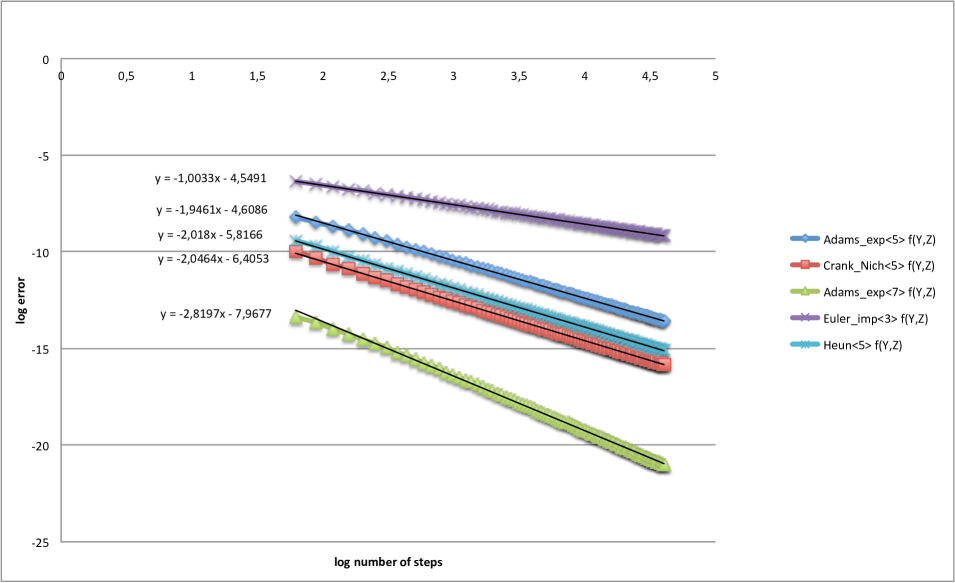
Figure 1: Illustration of the convergence rate

The graph in Fig. 2 below shows the impact of the space discretization on the global order of the method. The empirical convergence rates are in accordance with the theoretical ones.

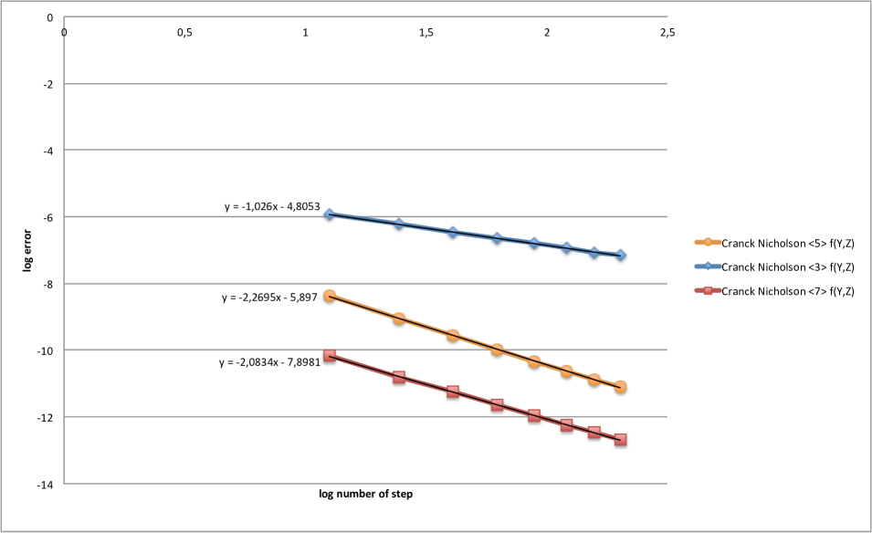
Figure 2: Impact of space discretization

4.3 Proof of Proposition 4.1

We only provide the proof of (i), the proof of (ii) follows from the same arguments and using the proof of Proposition 3.3 and Proposition 3.4.

1. Notations

We first need to consider ’functional’ version of the schemes above. Let us introduce the following operator, related to the theoretical schemes given in Definition 1.1.

$R^{Z}_{i,j}:(C^{1}_{b})^{2}\rightarrow C^{1}_{b}$

$$R^{Z}_{i,j}[\varphi^{Y},\varphi^{Z}](x)=\mathbb{E}\!\!\left[H^{\mathbf{1},x}_{t_{i},jh}\Big{(}\alpha_{j}\varphi^{Y}(W^{x,t_{i}}_{t_{i+j}})+h\beta_{j}f(\varphi^{Y}(W^{x,t_{i}}_{t_{i+j}}),\varphi^{Z}(W^{x,t_{i}}_{t_{i+j}}))\Big{)}\right]$$

$R^{Y}_{i,j}:(C^{1}_{b})^{2}\rightarrow C^{1}_{b}$

$$R^{Y}_{i,j}[\varphi^{Y},\varphi^{Z}](x)=\mathbb{E}\!\!\left[a_{j}\varphi^{Y}(W^{x,t_{i}}_{t_{i+j}})+hb_{j}f(\varphi^{Y}(W^{x,t_{i}}_{t_{i+j}}),\varphi^{Z}(W^{x,t_{i}}_{t_{i+j}}))\right]$$

Similarly, let us define - for the fully discrete scheme - the operators

$\widehat{R}^{Z}_{i,j}:(C^{1}_{b})^{2}\rightarrow C^{1}_{b}$

$$\widehat{R}^{Z}_{i,j}[\varphi^{Y},\varphi^{Z}](x)=\widehat{\mathbb{E}}\!\left[\widehat{H}_{i,j}\Big{(}\alpha_{j}\varphi^{Y}(\widehat{W}^{x,t_{i}}_{t_{ij}})+h\beta_{j}f(\varphi^{Y}(\widehat{W}^{x,t_{i}}_{t_{ij}}),\varphi^{Z}(\widehat{W}^{x,t_{i}}_{t_{ij}}))\Big{)}\right]$$

$\widehat{R}^{Y}_{i,j}:(C^{1}_{b})^{2}\rightarrow C^{1}_{b}$

$$\widehat{R}^{Y}_{i,j}[\varphi^{Y},\varphi^{Z}](x)=\widehat{\mathbb{E}}\!\left[a_{j}\varphi^{Y}(\widehat{W}^{x,t_{i}}_{t_{i+j}})+hb_{j}f(\varphi^{Y}(\widehat{W}^{x,t_{i}}_{t_{i+j}}),\varphi^{Z}(\widehat{W}^{x,t_{i}}_{t_{i+j}}))\right]$$

The functional version of the schemes given in Definition 4.1 reads then, for $i\leq n-r$,

$$\left\{\begin{array}[]{rcl}\widehat{y}_{i}(x)&=&\sum_{j=1}^{r}\widehat{R}^{Y}_{i,j}[\widehat{y}_{i+j},\widehat{z}_{i+j}](x)\vspace{2mm}\\ \widehat{z}_{i}(x)&=&\sum_{j=1}^{r}\widehat{R}^{Z}_{i,j}[\widehat{y}_{i+j},\widehat{z}_{i+j}](x)\end{array}\right.$$

given $r$ initial data $(\widehat{y}_{n-j},\widehat{z}_{n-j})=(u(t_{n-j},\cdot),\partial_{x}u(t_{n-j},\cdot))$, $0\leq j\leq r-1$.

Due to the markov property of the discrete process $(\widehat{W}^{0,x}_{t})_{t\in\pi}$, it is easily checked that

$$\widehat{Y}_{i}=\widehat{y}_{i}(\widehat{W}^{x,0}_{t_{i}})\text{ and }\widehat{Z}_{i}=\widehat{z}_{i}(\widehat{W}^{x,0}_{t_{i}})\;.$$

Finally, we define

$$\widetilde{Y}_{i}=u(t_{i},\widehat{W}^{x,0}_{t_{i}})\text{ and }\widetilde{Z}_{i}=\partial_{x}u(t_{i},\widehat{W}^{x,0}_{t_{i}})\;.$$

Observe that $\widetilde{Y}_{0}=u(0,x)$ and that, for $0\leq j\leq r-1$, $(\widehat{Y}_{n-j},\widehat{Z}_{n-j})=(\widetilde{Y}_{n-j},\widetilde{Z}_{n-j})$.

2. Stability

The key observation is here that $(\widetilde{Y}_{i},\widetilde{Z}_{i})$ can be seen as a perturbed version of the scheme given in (4.4), namely

$$\left\{\begin{array}[]{rcl}\widetilde{Y}_{i}&=&\widehat{\mathbb{E}}_{t_{i}}\!\left[\sum_{j=1}^{r}a_{j}\widetilde{Y}_{i+j}+h\sum_{j=0}^{r}b_{j}f(\widetilde{Y}_{i+j},\widetilde{Z}_{i+j})\right]+{}^{t}\zeta^{Y}_{i}+{}^{s}\zeta^{Y}_{i}\vspace{2mm}\\ \widetilde{Z}_{i}&=&\widehat{\mathbb{E}}_{t_{i}}\!\left[\sum_{j=1}^{r}H\Big{(}\alpha_{j}\widetilde{Y}_{i+j}+h\sum_{j=1}^{r}\beta_{j}f(\widetilde{Y}_{i+j},\widetilde{Z}_{i+j})\Big{)}\right]+{}^{t}\zeta^{Z}_{i}+{}^{s}\zeta^{Z}_{i}\end{array}\right.$$

where the local error due to the time-discretization is

$$\left\{\begin{array}[]{rcl}{}^{t}\zeta^{Y}_{i}&=&\mathbb{E}\!\!\left[Y_{t_{i}}-\check{Y}_{t_{i}}|X_{t_{i}}=\widehat{W}^{x,0}_{t_{i}}\right]\vspace{2mm}\\ {}^{t}\zeta^{Z}_{i}&=&\mathbb{E}\!\!\left[Z_{t_{i}}-\check{Z}_{t_{i}}|X_{t_{i}}=\widehat{W}^{x,0}_{t_{i}}\right]\end{array}\right.$$ (4.9)

recalling (2.11)-(2.12) and the local error due to the ’space-discretization’ is

$$\left\{\begin{array}[]{rcl}{}^{s}\zeta^{Y}_{i}&=&\sum_{j=1}^{r}(R^{Y}_{i,j}-\widehat{R}^{Y}_{i,j})[u(t_{i+j},\cdot),\partial_{x}u(t_{i+j},\cdot)](\widehat{W}^{x,0}_{t_{i}})\vspace{1mm}\\ {}^{s}\zeta^{Z}_{i}&=&\sum_{j=1}^{r}(R^{Z}_{i,j}-\widehat{R}^{Z}_{i,j})[u(t_{i+j},\cdot),\partial_{x}u(t_{i+j},\cdot)](\widehat{W}^{x,0}_{t_{i}})\end{array}\right..$$ (4.12)

Now, we can apply Proposition 2.1, recalling Remark 2.2, to obtain in particular that

$$|\widetilde{Y}_{0}-\widehat{Y}_{0}|^{2}\leq|\pi|\sum_{i=0}^{n-r}\widehat{\mathbb{E}}\!\left[\frac{1}{h_{i}^{2}}|{}^{t}\zeta^{Y}_{i}+{}^{s}\zeta^{Y}_{i}|^{2}+|{}^{t}\zeta^{Z}_{i}+{}^{s}\zeta^{Z}_{i}|^{2}\right]$$ (4.13)

3. Study of the local error

We now turn to the study of the local errors $(\zeta^{Y}_{i},\zeta^{Z}_{i})_{0\leq i\leq n-r}$. Assuming that the function are smooth enough we compute the following expansion

$$(R^{Y}_{i,j}-\widehat{R}^{Y}_{i,j})[u(t_{i+j},\cdot),u^{(1)}(t_{i+j},\cdot)](x)=\sum_{k=0}^{K}\frac{1}{k!}\chi^{(k)}_{i,j}(x)\mathbb{E}\!\!\left[(W^{0,t_{i}}_{t_{i+j}})^{k}\right] -\sum_{k=0}^{K}\frac{1}{k!}\chi^{(k)}_{i,j}(x)\widehat{\mathbb{E}}\!\left[(\widehat{W}^{0,t_{i}}_{t_{i+j}})^{k}\right]$$

$$+O(|\pi|^{\frac{K+1}{2}})$$

where $\chi_{i,j}$ are functions depending on $f$, $u$ and the coefficients of the methods.

Using the matching moment property of $\widehat{W}^{0,t_{i}}$, we easily obtain that

$$\widehat{\mathbb{E}}\!\left[|(R^{Y}_{i,j}-\widehat{R}^{Y}_{i,j})[u(t_{i+j},\cdot),u^{(1)}(t_{i+j},\cdot)](\widehat{W}^{x,0}_{t_{i}})|^{2}\right]\leq C|\pi|^{K+1}$$

For the $Z$ part, we have

$$(R^{Z}_{i,j}-\widehat{R}^{Z}_{i,j})[u(t_{i+j},\cdot),u^{(1)}(t_{i+j},\cdot)](x)=\sum_{k=0}^{K-1}\frac{1}{k!}\chi^{(k)}_{i,j}(x)\mathbb{E}\!\!\left[H_{i,j}(W^{0,t_{i}}_{t_{i+j}})^{k}\right] -\sum_{k=0}^{K-1}\frac{1}{k!}\chi^{(k)}_{i,j}(x)\widehat{\mathbb{E}}\!\left[(\widehat{H}_{i,j}\widehat{W}^{0,t_{i}}_{t_{i+j}})^{k}\right]$$

$$+O(|\pi|^{\frac{K-1}{2}})$$

Using the matching moment property of $\widehat{W}^{0,t_{i}}$, we easily obtain that

$$\widehat{\mathbb{E}}\!\left[|(R^{Z}_{i,j}-\widehat{R}^{Z}_{i,j})[u(t_{i+j},\cdot),u^{(1)}(t_{i+j},\cdot)](\widehat{W}^{x,0}_{t_{i}})|^{2}\right]\leq C|\pi|^{K-1}$$

Combining the above estimates with (4.13) and the fact that the discrete-time error is of order $m$, leads to

$$|\widetilde{Y}_{0}-\widehat{Y}_{0}|\leq C|\pi|^{m}+C|\pi|^{\frac{K-1}{2}}.$$

which concludes the proof since $K=2m+1$. $\Box$

References

- [1] Bally V. and G. Pagès (2003). Error analysis of the quantization algorithm for obstacle problems. Stochastic Processes and their Applications, 106, 1-40.
- [2] Bouchard B. and R. Elie (2008), Discrete-time approximation of decoupled forward-backward SDE with jumps, Stochastic Processes and their Applications, 118, 53-75.
- [3] Bouchard B. and N. Touzi (2004), Discrete-Time Approximation and Monte-Carlo Simulation of Backward Stochastic Differential Equations. Stochastic Processes and their Applications, 111 (2), 175-206.
- [4] Bouchard B. and X. Warin (2011) Monte-Carlo valorisation of American options: facts and new algorithms to improve existing methods, to appear in Numerical Methods in Finance , Springer Proceedings in Mathematics, ed. R. Carmona, P. Del Moral, P. Hu and N. Oudjane , 2011.
- [5] Butcher J. C. (2008), Numerical Methods for Ordinary Differential Equations, Second Edition, Wiley.
- [6] Chassagneux J.-F. (2008) Processus réfléchis en finance et probabilité numérique, phd thesis, Université Paris Diderot - Paris 7.
- [7] Chassagneux J.-F. and D. Crisan (2012), Runge-Kutta Scheme for BSDEs, preprint.
- [8] Crisan D. and K. Manolarakis (2009), Solving Backward Stochastic Differential Equations using the Cubature Method, preprint.
- [9] Crisan D. and K. Manolarakis (2010), Second order discretization of a Backward SDE and simulation with the cubature method, preprint.
- [10] Delarue, F. and S. Menozzi (2006) A forward backward algorithm for quasi-linear PDEs, Annals of Applied Probability ,16, 140-184.
- [11] Demailly J.-P. Analyse numérique et équations différentielles, 3e édition, EDP Sciences.
- [12] El Karoui N., S. Peng, M.C. Quenez (1997), Backward Stochastic Differential Equation in finance Mathematical finance, 7 (1), 1-71.
- [13] Gobet E. and C. Labart (2007), Error expansion for the discretization of bacward stochastic differential equations, Stochastic Processes and their Applications, 117, 803-829.
- [14] Gobet E., J.-P. Lemor and X. Warin (2006) Rate of convergence of an empirical regression method for solving generalized backward stochastic differential equations, Bernoulli, 12(5), 889-916.
- [15] Kloeden P. E. and E. Platen (1992), Numerical solutions of Stochastic Differential Equations, Applied Math. 23, Springer, Berlin.
- [16] Pardoux E. and S. Peng (1990), Adapted solution of a backward stochastic differential equation, Systems and Control Letters, 14, 55-61.
- [17] Pardoux E. and S. Peng (1992), Backward stochastic differential equations and quasilinear parabolic partial differential equations. In Stochastic partial differential equations and their applications (Charlotte, NC, 1991), 200-217, volume 176 of Lecture Notes in Control and Inform. Sci., Springer, Berlin, 1992.
- [18] Richou, A. (2010) Numerical simulation of BSDEs with drivers of quadratic growth. Forthcoming in The Annals of Applied Probability.
- [19] Zhao W., L. Chen and S. Peng (2006), A new kind of accurate numerical method for backward stochastic differential equations, SIAM J. Sci. Comput., 28, 1563-1581.
- [20] Zhao W., Y. Li and G. Zhang, (2012) A generalized theta-scheme for solving backward stochastic differential equations , Dis. Cont. Dyn. Sys. B, 117, 1585-1603.
- [21] Zhao W., J. Wang and S. Peng (2009) Error estimates of the theta-scheme for backward stochastic differential equations , Dis. Cont. Dyn. Sys. B, 12, 905-924.
- [22] Zhao W., G. Zhang and L. Ju (2010) A stable multistep scheme for solving Backward Stochastic Differential Equations. SIAM J. Numer. Anal. 48(4), 1369-1394.
- [23] Zhang J. (2004), A numerical scheme for backward stochastic differential equation, Annals of Applied Probability, 14(1), 459-488.