Long range correlations and folding angle in polymers
with applications to $\alpha$-helical proteins

Abstract

The conformational complexity of linear polymers far exceeds that of point-like atoms and molecules. Polymers can bend, twist, even become knotted. Thus they may also display a much richer phase structure than point particles. But it is not very easy to characterize the phase of a polymer. Essentially, the only attribute is the radius of gyration. The way how it changes when the degree of polymerization becomes different, and how it evolves when the ambient temperature and solvent properties change, discloses the phase of the polymer. Moreover, in any finite length chain there are corrections to scaling, that complicate the detailed analysis of the phase structure. Here we introduce a quantity that we call the folding angle, a novel tool to identify and scrutinize the phases of polymers. We argue for a mean-field relationship between its values and those of the scaling exponent in the radius of gyration. But unlike in the case of the radius of gyration, the value of the folding angle can be evaluated from a single structure. As an example we estimate the value of the folding angle in the case of crystallographic $\alpha$-helical protein structures in the Protein Data Bank (PDB). We also show how the value can be numerically computed using a theoretical model of $\alpha$-helical chiral homopolymers.

Despite substantial differences in their chemical composition, all linear polymers are presumed to share the same universal phase structure degennes ; schafer ; naka . But the phase where a particular polymer resides depends on many factors including polymer concentration, the quality of solvent, ambient temperature and pressure. Three phases are commonly identified, each of them categorized by the manner how the polymer fills the space degennes ; schafer ; naka ; naka2 : If the solvent is poor and the attractive interactions between monomers dominate, a single polymer chain is presumed to collapse into a space-filling conformation. In a good solvent environment or at sufficiently high temperatures, a single polymer chain tends to swell until its geometric structure bears similarity to a self-avoiding random walk (SARW). The collapsed phase and the SARW phase are separated by $\Theta$-point where a polymer has the characteristics of an ordinary random walk (RW). Biologically active proteins are commonly presumed to reside in the space filling collapsed phase, under physiological conditions. We shall examine proteins as an important subset of polymers, for which a large amount of experimental data is available in PDB pdb .

The phase where a polymer resides can be determined from the value of the scaling exponent $\nu$ degennes ; schafer ; naka . To define this quantity, we consider the asymptotic behavior of the radius of gyration when the number of monomers $N$ is very large. With ${\bf r}_{i}$ the coordinates of the skeletal atoms of the polymer, the radius of gyration becomes in this limit degennes ; schafer ; naka ; degen2 ; desc ; sokal

$$R_{g}\ =\ \sqrt{\,\frac{1}{2N^{2}}\sum_{i,j}({\bf r}_{i}-{\bf r}_{j})^{2}\,}\ \buildrel N\ {\rm large}\over{\longrightarrow}\ R_{0}N^{\nu}+\dots$$ (1)

The length scale $R_{0}$ is an effective Kuhn distance between the skeletal atoms in the large-$N$ limit. It is in principle a computable quantity, that depends on all the atomic level details of the polymer and all the effects of environment including pressure, temperature and chemical microstructure of the solvent. Unlike $R_{0}$, the dimensionless scaling exponent $\nu$ that governs the large-$N$ asymptotic form of equation (1), is a universal quantity. Its numerical value is independent of the local atomic level structure, and coincides with the inverse of the Hausdorff (fractal) dimension $d_{H}$ of the polymer. The numerical value of $\nu=1/d_{H}$ serves as an order parameter of polymer phase structure:

For a continuous self-nonintersecting chain in three space dimensions $d_{H}$ can in principle acquire any value between 1 and 3. Simple examples of fractal structures where $d_{H}$ is not an integer, include the piecewise linear Koch curve and attractors of chaotic equations such as the Lorenz and the Rössler equations chaos .

The phases of polymers and in particular proteins, have been presumed to display fractal geometry frac0 ; frac1 ; dewey ; frac2 ; frac3 ; dima ; frac4 ; hong ; huang ; jcp ; scheraga . Traditionally, the following values of $\nu$ are assigned to these phases degennes ; schafer : Biologically active proteins are commonly in the space filling $d_{H}=3$ phase. For the $\Theta$-point $d_{H}=2$, and for the SARW phase the Flory-Huggins value $d_{H}=5/3$ is found huggins , flory .

.

In analyses of PDB proteins, additional values of $\nu$ have been proposed dewey -scheraga . For example, hong argues for the scaling exponent $\nu=2/5$ instead of $1/3$ for the collapsed phase. Moreover, according to dewey , hong the value of $\nu$ depends on the type of the protein, different values are quoted for different fold types such as all-$\alpha$ proteins, all-$\beta$ proteins, and $\alpha/\beta$ proteins. Furthermore, huang argues that protein folding involves three stages: The Flory-Huggins value $\nu=3/5$ proceeds to an intermediate phase with $\nu=3/7$, followed by $\nu=2/5$ in the collapsed state. According to jcp for unstructured proteins the scaling exponent has the value $\nu=0.43\pm 0.02$.

In this Letter we introduce a novel geometric characteristic of polymer phase structure, that we call the folding angle. It is complementary to the scaling index $\nu$ and might provide certain advantages: Unlike $\nu$ it can, in principle, be computed from a single structure. Moreover, (1) is known to be subject to very strong finite-size effects; in the SARW phase sokal detects corrections to $\nu$ whenever $N$ is less than $N\sim 10^{4}$. Consequently, in the case of proteins where $N$ is much smaller, the presence of potentially strong corrections to scaling effects in the value of $\nu$ should not be ignored. The relation between $\nu$ and the folding angle could be a useful tool to try and estimate these corrections.

We consider a polymer backbone with skeletal atoms at $\mathbf{r}_{i}$. We define the unit length tangent ($\mathbf{t}$) and bi-normal ($\mathbf{b}$) vectors at each site $i=1,...,N$,

$$\mathbf{t}_{i}\ =\ \frac{\mathbf{r}_{i+1}-\mathbf{r}_{i}}{|\mathbf{r}_{i+1}-\mathbf{r}_{i}|}\ \ \ \ \&\ \ \ \ \mathbf{b}_{i}\ =\ \frac{\mathbf{t}_{i-1}\times\mathbf{t}_{i}}{|\mathbf{t}_{i-1}\times\mathbf{t}_{i}|}$$ (2)

The backbone bond ($\kappa$) and torsion ($\tau$) angles are

$$\mathbf{t}_{i+1}\cdot\mathbf{t}_{i}\ =\ \cos\kappa_{i}\ \ \ \ \ \&\ \ \ \ \ \mathbf{b}_{i+1}\cdot\mathbf{b}_{i}\ =\ \cos\tau_{i}$$ (3)

We assume that $N$ is very large. We introduce a block-spin transformation which at each step number $p$ combines two (or more) skeletal subunits into a new subunit; see Figure 1. We introduce the new tangent vectors, corresponding to the new subunits, by setting

$$\mathbf{t}^{(p)}_{i}\ \to\ \frac{\mathbf{t}^{(p)}_{2j-1}+\mathbf{t}^{(p)}_{2j}}{|\mathbf{t}^{(p)}_{2j-1}+\mathbf{t}^{(p)}_{2j}|}\ =\ \mathbf{t}_{j}^{(p+1)}$$

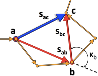
Figure 1: (Color online) Two steps in the block-spin transformation that we utilize in evaluating (4).

This gives new coarse-grained bond angles,

$$\cos\,\kappa_{i}^{{(p)}}=\mathbf{t}^{(p)}_{i+1}\cdot\mathbf{t}^{(p)}_{i}\to\,\mathbf{t}_{j+1}^{{(p+1)}}\cdot\mathbf{t}_{j}^{{(p+1)}}\!=\cos\,\kappa_{j}^{{(p+1)}}$$

We assume that when we repeat this transformation a very large number $p$ of times, the numerical values of the transformed bond angles $\kappa^{(p)}_{i}$ converge towards a single fixed point value $\kappa^{\star}$,

$$<\!\mathbf{t}^{(p)}_{i}\cdot\mathbf{t}^{(p)}_{i+1}\!>\ \buildrel p\to\infty\over{\longrightarrow}\ \cos\kappa^{\star}$$ (4)

This is commonly the case for self-similar chains. We call $\kappa^{\star}$ the folding angle and propose that the numerical value of (4) depends only on the phase of polymer.

We first argue that when the limit (4) exists and is unique, there is the following asymptotic $p\to\infty$ relation between the cosine of $\kappa^{\star}$ and the scaling exponent $\nu$,

$$\cos\kappa^{\star}\approx\ 2^{2\nu-1}-1$$ (5)

$$\Rightarrow\ \cos\kappa^{\star}\ =\ \left\{\,\begin{matrix}-0.21\ \dots&\hskip-62.59596pt\,\nu=1/3\\ \hskip-22.76228pt0&\hskip-59.75095pt\nu=1/2\\ \hskip 5.69046pt0.11\ \dots&\hskip 0.0pt\nu=0.5888\dots\ \sim 3/5\end{matrix}\right.$$ (6)

The SARW estimate is taken from sokal and $3/5$ is the corresponding Flory-Huggins result huggins , flory . Note that the $\Theta$-point value $\nu=1/2$ is exact: At the $\Theta$-point where long range correlations along the chain are absent, standard arguments degennes imply that (4) must vanish. The value for $\nu=1/3$ is similarly exact, for a space filling structure.

To justify (5), (6) we consider a polymer chain where we have implemented the block-spin transformation several times, to arrive at a configuration where three consecutive nearest neighbor skeletal subunits that we denote by $a,b,c$ are connected by vectors $\mathbf{s}_{ab}$ and $\mathbf{s}_{bc}$ as shown in Figure 1. We introduce the next block-spin transformation. As shown in Figure 1, it replaces these two vectors with the vector $\mathbf{s}_{ac}$. We consider a statistical ensemble of the polymer, and compute the ensemble average of the squared length of the vector $\mathbf{s}_{ac}$. The result is

$$<\!\mathbf{s}_{ac}^{2}\!>\,=\,<\!\mathbf{s}_{ab}^{2}\!>+<\!\mathbf{s}_{bc}^{2}\!>+2<\!|\mathbf{s}_{ab}|\,|\mathbf{s}_{bc}|\cos\kappa_{b}\!>$$

Consider the scaling limit where the block-spin subunits consist of $n$ skeletal atoms, where $n$ is large. Assume that the polymer is in a phase where the distances $s_{ab}$, $s_{bc}$ and $s_{ac}$ scale according to (1), that is

$$<\!\mathbf{s}_{ab}^{2}\!>\,\sim\,<\!\mathbf{s}_{bc}^{2}\!>\,\sim\,n^{2\nu}\ \ \ \&\ \ \ <\!\mathbf{s}_{ac}^{2}\!>\,\sim\,(2n)^{2\nu}$$

Note that $\mathbf{s}_{ac}$ corresponds to the step where the skeletal subunit consists of $2n$ original atomic skeletals while both $\mathbf{s}_{ab}$ and $\mathbf{s}_{bc}$ are constructed with $n$ atomic skeletals. We now assume that to leading order in $n$ the ensemble averages factorize, so that we have

$$<\!|\mathbf{s}_{ab}|\,|\mathbf{s}_{bc}|\cos\kappa_{b}\!>\,\sim\,<\!|\mathbf{s}_{ab}|\!><\!|\mathbf{s}_{bc}|\!><\!\cos\kappa_{b}\!>+\mathcal{O}(\frac{1}{n})$$

From this we immediately obtain (4) and (5), when we identify $\mathbf{t}_{i}^{ren}$ with the unit vector in the direction $\mathbf{s}_{ab}$.

Note that (5) engages an exponential in $\nu$. Thus $\cos\kappa^{\star}$ might indeed be more sensitive than $\nu$, in characterizing corrections to scaling.

We first estimate $\cos\kappa^{\star}$, in the case of PDB protein structures pdb . Here space allows us to analyze in detail only the subset of mainly $\alpha$-helical proteins in the CATH classification cath ; the issues raised in dewey -jcp will be addressed elsewhere. We consider those $\alpha$-helical proteins in PDB with less than $30\%$ homology identity, and single chain in biological assembly. There are a total of 1174 structures in our data set, and this enables us to reliably extend our analysis to $2n=330$ residues. The result is shown in Figure 2. We find that when $2n\sim 330$

$$<\!\cos\kappa^{\star}\!>\approx-0.18\dots$$ (7)

which corresponds to $\nu\approx 0.357\dots\$ according to (5). This is remarkably close to the value $\nu=1/3$ in (6), for a fully space filling configuration. For comparison, using the radius of gyration fit to the all-$\alpha$ PDB structures, hong finds $\nu\approx 0.403$ while scheraga reports $\nu\approx 0.37$ for these structures.

We observe in Figure 2 that when $n$ is very small, $\cos\kappa^{\star}$ tends to have (mainly) positive values. Over a very short distance of only a few amino acids, the structure is determined by the covalent bonds. Indeed, due to steric constraints, the virtual C_α backbone bond angle is known to prefer values that are less than $\pi/2$ marty1 ; marty2 . When the number of residues $n$ increases the backbone starts pulling together, (4) decreases and becomes negative foot . When $n$ increases further, excluded volume effects come into play. This causes a dense-backing repulsion, the value of (4) starts increasing, converging towards the asymptotic value (7).

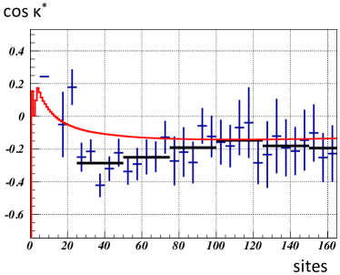
Figure 2: (Color online) (Blue) entries denote distribution (4) in our PDB data, described in the text. The averages are over $\Delta N=5$ bins. (Black) horizontal lines are piecewise linear interpolations that average the PDB data, over $\Delta N=25$ bins, weighted over the number of PDB entries. Continuous (red) line is the result of theoretical computation using (8).

For a theoretical estimate of (4), we need a dynamical model. We have chosen the following Hamiltonian free energy ulf -martin .

$$E=\sum\limits_{i=1}^{N}\biggl{\{}-2\kappa_{i+1}\kappa_{i}+2\kappa_{i}^{2}+c(\kappa_{i}^{2}-m^{2})^{2}+b\kappa_{i}^{2}\tau_{i}^{2}\biggr{\}}\ +\ \sum\limits_{i=1}^{N}\biggl{\{}d\tau_{i}+e\tau_{i}^{2}\biggr{\}}\ \ \ \ \ \ \ (\kappa_{N+1}=0)$$ (8)

It describes collapsed chiral homopolymers as local energy minima in terms of the backbone bond and torsion angles. The detailed derivation of (8) can be found in ying . Here it suffices to state that the energy function (8) can be shown to be a long-distance limit that describes the full microscopic energy of a folded protein scheraga . As such, it does not explain the details of the (sub-)atomic level mechanisms that give rise to protein folding. In applications to polymers we need to complement (8) by the excluded volume constraint, due to steric repulsions. We demand that the chain we construct using the ($\kappa_{i},\tau_{i}$) values in (8) by inverting (3) and (2), is subject to

$$|\mathbf{r}_{i}-\mathbf{r}_{j}|>\Delta\ \ \ \ \ i\not=j$$ (9)

In the case of proteins we choose $\Delta=3.8~{}{\rm\AA}$, the average distance between two neighboring $C_{\alpha}$ atoms.

To compute the result shown by the red curve in Figure 2 we introduce a finite temperature environment using a canonical ensemble, and evaluate the ensuing Bolzmannian partition function numerically by Monte Carlo integration. We have collected statistics over a period of around three months of wall-clock time, using a 120 processor MacPro desktop farm; the error-bars are minuscule and thus not displayed in Figure 2. In our simulations we thermalize each chain during 10 million Monte Carlo steps with the following parameter values, $c=5.4$, $m=1.51$, $b=0.02$, $d=-0.09$, $e=-0.001$. These parameters are chosen so that the minimum energy configurations are like $\alpha$-helical protein structures nora ; andrei1 ; martin ; we have checked that our results are quite insensitive to the choice of parameter values, and do not change if the number of Monte Carlo steps is increased.

From Figure 2 we observe that qualitatively, our numerical results and the experimental PDB data are quite similar: For very small values on $n$, (4) is positive. It then starts decreasing and becomes negative. There is a minimum value, at $n_{min}\approx 110$. After this (4) starts increasing towards its asymptotic negative value of the scaling limit. For long chains $2n\sim 320$ we find

$$<\cos\kappa^{\star}>\ =\ -0.14...$$ (10)

corresponding to $\nu\approx 0.391\dots$ when we use (5). This is between the values $\nu\approx 0.403$ and $\nu\approx 0.37$ reported in hong ; scheraga respectively, for all-$\alpha$ proteins in PDB, obtained by using (1).

We have also estimated (5) from (8) in the self-avoiding random walk phase, using an ensemble of chains with fixed length $2n=500$. In the high temperature limit the energy does not contribute, only (9) is relevant, and we find

$$<\!\cos\kappa^{\star}\!>\ \approx\,+\,0.10...$$

From (5) we now get $\nu\approx 0.57$ which is very close to the SARW value $\sim 0.5888\ \dots$ obtained in sokal for chains with $n\sim 10^{5}$.

In summary, we have introduced the concept of folding angle as a new tool to characterize the phases of polymers. We have proposed a relation between the cosine of the folding angle and the scaling exponent of the radius of gyration, that we have investigated using both experimental data and model dependent numerical simulations. Unlike the scaling exponent the cosine of the folding angle can, in principle, be computed from a single configuration. The results also propose that the cosine of the folding angle could better reveal the presence of corrections to scaling in the vicinity of the collapsed state fixed point, than the scaling exponent. Thus we expect that the folding angle can become a valuable new order parameter in understanding the phase structure of polymers.

We acknowledge support from CNRS PEPS Grant, Region Centre Recherche d^′Initiative Academique grant, Sino-French Cai Yuanpei Exchange Program, and Qian Ren Grant at BIT.

References

- (1) P.G. DeGennes, Scaling Concepts in Polymer Physics (Cornell University Press, Ithaca, 1979)
- (2) L. Schäfer, Excluded Volume Effects in Polymer So- lutions, as Explained by the Renormalization Group (Springer Verlag, Berlin, 1999)
- (3) T. Nakayama, Y. Kousuke, R.L. Orbach Rev. Mod. Phys. 66 381 (1994)
- (4) Additional criteria include the density of vibrational states, and the probability of a random walker to be found at the point of origin as a function of time naka .
- (5) H.M. Berman, et.al Nucl. Acids Res. 28 235 (2000); http://www.pdb.org
- (6) P.G. DeGennes, Phys. Lett A38 339 (1972)
- (7) J. Des Cloizeaux, J. Phys. (Paris) 36 281 (1975)
- (8) B. Li, N. Madras, A. Sokal, Journ. Stat. Phys. 80 661 (1995).
- (9) see for example S.H. Strogatz, Nonlinear Dynamics and Chaos - With Applications to Physics, Biology, Chemistry and Engineering (Perseus Books, Cambridge, MA, 1994)
- (10) H.J. Stapleton, J.P. Allen, C.P. Flynn, D.G. Stinson, S.R. Kurtz Phys. Rev. Lett. 45 1456 (1980)
- (11) 16. R. Elber, M. Karplus, Phys. Rev. Lett. 56 394 (1986)
- (12) T.G. Dewey, Journ. Chem. Phys. 98 2250 (1993)
- (13) X. Yu, D.M. Leitner, Journ. Chem. Phys. 119 12673 (2003)
- (14) R. Burioni, D. Cassi, F. Cecconi, A. Vulpiani, Proteins 55 529 (2004)
- (15) R.I. Dima, D. Thirumalai, J. Phys. Chem. B 108, 6564 (2004).
- (16) M.B. Enright, D.M. Leitner Phys. Rev. E71 011912 (2005)
- (17) L. Hong, J. Lei, Polym. Sci. B47 207 (2009)
- (18) J. Lei, K. Huang, EPL 88 68004 (2009)
- (19) N. Rawat, P. Biswas, Journ. Chem. Phys. 131 065104 (2009)
- (20) A. Krokhotin, A. Liwo, A.J. Niemi, H.A. Scheraga, Journ. Chem. Phys. 137 035101 (2012)
- (21) M.L. Huggins, Journ. Chem. Phys. 9 440 (1941)
- (22) P.J. Flory, Journ. Chem. Phys. 9 660 (1941).
- (23) C.A. Orengo, et.al Structure 5 1093 (1997); http://www.cathdb.info/
- (24) M. Lundgren, A.J. Niemi, F. Sha, Phys. Rev. E85 061909 (2012)
- (25) M. Lundgren, A.J. Niemi, Phys. Rev. E86 021904 (2012)
- (26) For three consecutive amino acids excluded volume constraint gives the lower bound .
- (27) U. Danielsson, M. Lundgren, A.J. Niemi, Phys. Rev. E82 021910 (2010)
- (28) N.Molkenthin, S. Hu, A.J. Niemi Phys. Rev. Lett. 106 078102 (2011)
- (29) S. Hu, Y. Jiang, A.J. Niemi, Phys. Rev. D87 105011 (2013)
- (30) A. Krokhotin, A.J. Niemi, X. Peng, Phys. Rev. E85 031906 (2012)
- (31) A. Krokhotin, M. Lundgren, A.J. Niemi, Phys. Rev. E86 021923 (2012)