Analysis of Boundary Conditions
for Crystal Defect Atomistic Simulations

Abstract.

Numerical simulations of crystal defects are necessarily restricted to finite computational domains, supplying artificial boundary conditions that emulate the effect of embedding the defect in an effectively infinite crystalline environment. This work develops a rigorous framework within which the accuracy of different types of boundary conditions can be precisely assessed.

We formulate the equilibration of crystal defects as variational problems in a discrete energy space and establish qualitatively sharp regularity estimates for minimisers. Using this foundation we then present rigorous error estimates for (i) a truncation method (Dirichlet boundary conditions), (ii) periodic boundary conditions, (iii) boundary conditions from linear elasticity, and (iv) boundary conditions from nonlinear elasticity. Numerical results confirm the sharpness of the analysis.

1. Introduction

Crystalline solids can contain many types of defects. Two of the most important classes are dislocations, which give rise to plastic flow, and point defects, which can affect both elastic and plastic material behaviour as well as brittleness.

Determining defect geometries and defect energies are a key problem of computational materials science [46, Ch. 6]. Defects generally distort the host lattice, thus generating long-ranging elastic fields. Since practical schemes necessarily work in small computational domains (e.g., “supercells”) they cannot explicitly resolve these fields but must employ artificial boundary conditions (periodic boundary conditions appear to be the most common). To assess the accuracy and in particular the cell size effects of such simulations, numerous formal results, numerical explorations, or results for linearised problems can be found in the literature; see e.g. [3, 16, 26, 8] and references therein for a small representative sample.

The novelty of the present work is that we rigorously establish explicit convergence rates in terms of computational cell size, taking into account the long-ranged elastic fields. Our framework encompasses both point defects and straight dislocation lines. Related results in a PDE context have recently been developed in [5].

The second motivation for our work is the analysis of multiscale methods. Several multiscale methods have been proposed to accelerate crystal defect computations (for example atomistic/continuum coupling [29], [24] or QM/MM [4]), and our framework provides a natural set of benchmark problems and a comprehensive analytical substructure for these methods to assess their relative accuracy and efficiency. In particular, it provides a machinery for the optimisation of the (non-trivial) set of approximation parameters in multiscale schemes.

The mathematical analysis of crystalline defects has traditionally focused on dislocations [17, 2, 1, 19] and on electronic structure models [11, 10]; however, see [9] for a comprehensive recent review focused on point defects. The results in the present work, in particular the decay estimates on elastic fields, also have a bearing on this literature since they can be used to establish finer information about equilibrium configurations; see e.g., [20].

Acknowledgement

We thank Brian Van Koten who pointed out a substantial flaw in our construction of the edge dislocation predictor in an earlier version of this work, and made valuable comments that helped us resolve it.

1.1. Outline

Our approach consists in placing the defect in an infinite crystalline environment, for simplicity say $\mathbb{Z}^{d}$, where $d\in\{2,3\}$ is the space dimension, applying a far-field boundary condition which encodes the macroscopic state of the system within which the defect is embedded. Let $w:\mathbb{Z}^{d}\to\mathbb{R}^{m}$ be the unknown displacement of the crystal, then we decompose $w=u_{0}+u$, where $u_{0}$ is a predictor that specifies the boundary condition through the requirement that the corrector $u$ belongs to a discrete energy space $\dot{\mathscr{W}}^{1,2}$ (a canonical discrete variant of $\dot{H}^{1}(\mathbb{R}^{d})$). We then formulate the condition for $w$ to be an equilibrium configuration as a (local) energy minimisation problem,

$$\bar{u}\in\arg\min\big{\{}\mathscr{E}(u)\,\big{|}\,u\in\dot{\mathscr{W}}^{1,2}\big{\}},$$ (1.1)

where $\mathscr{E}(u)$ is the energy difference between the total displacement $w=u_{0}+u$ and the predictor $u_{0}$.

The choice of $u_{0}$ is not arbitrary. It is crucial that $u_{0}$ is an “approximate equilibrium” in the far-field, which will be expressed through the requirement that $\delta\mathscr{E}(0)\in(\dot{\mathscr{W}}^{1,2})^{*}$. It is clear that, if this condition fails, then $\inf\{\mathscr{E}(u)\,|\,u\in\dot{\mathscr{W}}^{1,2}\}=-\infty$. For this reason, we think of $u_{0}$ as a predictor and $u$ as a corrector. For the case of dislocations, the choice of $u_{0}$ is non-trivial, as the “naive” linear elasticity predictor does not take lattice symmetries correctly into account. In § 3.1 we present a new construction that remedies this issue.

We shall not be concerned with existence of solutions to (1.1); even for the simplest classes of defects this is a difficult problem. Uniqueness can never be expected for realistic interatomic potentials.

However, assuming that a solution to (1.1) does exist, we may then analyze its “regularity”. More precisely, under a natural stability assumption we estimate the rate in terms of distance to the defect core at which $\bar{u}$ (and its discrete gradients of arbitrary order) approach zero. For example, we will prove that

$$|D\bar{u}(\ell)|\leq C|\ell|^{-d}(\log|\ell|)^{r},$$

where $Du(\ell)$ is a finite difference gradient centered at $\ell\in\mathbb{Z}^{d}$, $r=0$ for point defects and $r=1$ for straight dislocation lines.

These regularity estimates then allow us to establish various approximation results. For example, we can estimate the error committed by projecting an infinite lattice displacement field $u$ to a finite domain by truncation. This motivates the formulation of a Galerkin-type approximation scheme for (1.1) (see § 2.3 and § 3.4)

$$\bar{u}_{N} \in\arg\min\big{\{}\mathscr{E}(u)\,\big{|}\,u\in\dot{\mathscr{W}}^{1,2}_{N}\big{\}},$$ (1.2)

$$\text{where}\quad\dot{\mathscr{W}}^{1,2}_{N}:=\big{\{}u\in\dot{\mathscr{W}}^{1,2}\,\big{|}\,u(\ell)=0\text{ for }|\ell|\geq N^{1/d}\big{\}}.$$

This is a finite dimensional optimisation problem with ${\rm dim}(\dot{\mathscr{W}}^{1,2}_{N})\approx N$, and our framework yields a straightforward proof of the following error estimate: suppose $\bar{u}$ is a strongly stable (cf. (2.6)) solution to (1.1) then, for $N$ sufficiently large, there exists a solution $\bar{u}_{N}$ to (1.2) such that

$$\|\bar{u}-\bar{u}_{N}\|_{\dot{\mathscr{W}}^{1,2}}\leq CN^{-1/2}(\log N)^{r},$$

where $r=0$ for point defects, $r=1/2$ for straight dislocation lines, and $\|\bar{u}-\bar{u}_{N}\|_{\dot{\mathscr{W}}^{1,2}}$ is a natural discrete energy norm. Note that $N$ is directly proportional to the (idealised) computational cost of solving (1.2). We stress that we stated only that “there exists a $\bar{u}_{N}$”; indeed, both (1.1) and (1.2) typically have many solutions. Roughly speaking, this means that “near every stable solution to (1.1) there exists a stable solution to (1.2)”. It is interesting to note that the rate $N^{-1/2}$ is generic; that is, it is independent of any details of the particular defect. We prove a similar error estimate for periodic boundary conditions in § 2.4.

In §§ 2.5, 2.6, 3.6, 3.7 we then consider two types of concurrent (or, self-consistent) boundary conditions that use elasticity models to improve the far field corrector. In these approximate models, we solve a far-field problem concurrently with the atomistic core problem in order to improve the boundary conditions placed on the atomistic core. First, in § 2.5, 3.6 we use linearised lattice elasticity to construct an improved far-field predictor. Second, in § 2.6, 3.7 we analyze the effect of using nonlinear continuum elasticity to improve the far-field boundary condition. This effectively leads us to formulate an atomistic-to-continuum coupling scheme within our framework. For both methods we show that, in the point defect case this yields substantial improvements over the simple truncation method, but surprisingly, for dislocations the methods are qualitatively comparable to the simple truncation scheme. We note, however that based on the benchmarks of the present paper, improved a/c schemes with superior convergence rates have recently been developed in [23, 35].

Our numerical experiments in § 2.7, 3.8 mostly confirm that our analytical predictions are sharp, however, we also show some cases where they do not capture the full complexity of the convergence behaviour.

Restrictions

Our analysis in the present paper is restricted to static equilibria under classical interatomic interaction with finite interaction range. We see no obstacle to include Lennard-Jones type interactions, but this would require finer estimates and a more complex notation. However, we explicitly exclude Coulomb interactions or any electronic structure model and hence also charged defects (see, e.g., [16, 26, 11, 10, 9]). Due to the computational cost involved in these latter models, obtaining analogous convergence results for these, would be of considerable interest.

As reference atomistic structure we admit only single-species Bravais lattices. Again, we see no conceptual obstacles to generalising to multi-lattices, however, some of the technical details may require additional work.

As already mentioned we only focus on “compactly supported” defects, but exclude curved line defects, grain or phase boundaries, surfaces or cracks. Moreover, we exclude the case of multiple or indeed infinitely many defects. We hope, however, that our new analytical results on single defects will aid future studies of this setting; e.g., see [20] for an analysis of multiple screw dislocations which is based on the present work.

Notation

Notation is introduced throughout the article. Key symbols that are used across sections are listed in Appendix C. We only briefly remark on some generic points. The symbol $\langle\cdot,\cdot\rangle$ denotes an abstract duality pairing between a Banach space and its dual. The symbol $|\cdot|$ normally denotes the Euclidean or Frobenius norm, while $\|\cdot\|$ denotes an operator norm.

The constant $C$ is a generic positive constant that may change from one line of an estimate to the next. When estimating rates of decay or convergence rates then $C$ will always remain independent of approximation parameters (such as $N$, which relates to domain size), of lattice position (such as $\ell$) or of test functions. However, it may depend on the interatomic potential or some fixed displacement or deformation field (e.g., on the boundary condition and the solution). The dependencies of $C$ will normally be clear from the context, or stated explicitly. To improve readability, we will sometimes replace $\leq C$ with $\lesssim$.

For a differentiable function $f$, $\nabla f$ denotes the Jacobi matrix and $\nabla_{r}f=\nabla f\cdot r$ the directional derivative. The first and second variations of a functional $E\in C^{2}(X)$ are denoted, respectively, by $\langle\delta E(u),v\rangle$ and $\langle\delta^{2}E(u)w,v\rangle$ for $u,v,w\in X$. We will avoid use of higher variations in this explicit way.

If $\Lambda\subset\mathbb{R}^{d}$ is a discrete set and $u:\Lambda\to\mathbb{R}^{m}$, $\ell\in\Lambda$ and $\ell+\rho\in\Lambda$, then we define the finite difference $D_{\rho}u(\ell):=u(\ell+\rho)-u(\ell)$. If $\mathcal{R}\subset\Lambda-\ell$, then we define $D_{\mathcal{R}}u(\ell):=(D_{\rho}u(\ell))_{\rho\in\mathcal{R}}$. We will normally specify a specific stencil $\mathcal{R}_{\ell}$ associated with a site $\ell$ and define $Du(\ell):=D_{\mathcal{R}_{\ell}}u(\ell)$. For ${\bm{\rho}}\in(\mathcal{R}_{\ell})^{j}$, $D_{\bm{\rho}}u:=D_{\rho_{1}}\ldots D_{\rho_{j}}u$ denotes a $j$-th order derivative, and $D^{j}u$ defined recursively by $D^{j}u:=DD^{j-1}u$ denotes the $j$-th order collection of derivatives.

2. Point Defects

2.1. Atomistic Model

We formulate a model for a point defect embedded in a homogeneous lattice. To simplify the presentation, we admit only a finite interaction radius (in reference coordinates) and a smooth interatomic potential. Both are easily lifted, but introduce non-essential technical complications.

Let $d\in\{2,3\}$ and ${\sf A}\in\mathbb{R}^{d\times d}$ nonsingular, defining a Bravais lattice ${\sf A}\mathbb{Z}^{d}$. The reference configuration for the defect is a set $\Lambda\subset\mathbb{R}^{d}$ such that, for some ${R_{\rm def}}>0$, $\Lambda\setminus B_{{R_{\rm def}}}={\sf A}\mathbb{Z}^{d}\setminus B_{{R_{\rm def}}}$ and $\Lambda\cap B_{{R_{\rm def}}}$ is finite. For analytical purposes it is convenient to assume the existence of a background mesh, that is, a regular partition $\mathcal{T}_{\Lambda}$ of $\mathbb{R}^{d}$ into triangles if $d=2$ and tetrahedra if $d=3$ whose nodes are the reference sites $\Lambda$, and which is homogeneous in $\mathbb{R}^{d}\setminus B_{{R_{\rm def}}}$. (If $T\in\mathcal{T}_{\Lambda}$ and $\rho\in{\sf A}\mathbb{Z}^{d}$ with $T,\rho+T\subset\mathbb{R}^{d}\setminus B_{{R_{\rm def}}}$, then $\rho+T\in\mathcal{T}_{\Lambda}$ as well.) We refer to Figure 1 for two-dimensional examples of such triangulations.

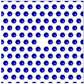
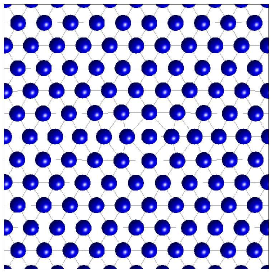
(a)                                                        (b)

Figure 1. Illustration of (a) vacancy and (b) interstitial defects; relaxed configurations computed with ATM-DIR (cf. § 2.7). The grey lines indicate the interaction bonds, $\mathcal{R}_{\ell}$, between atoms, for a nearest-neighbour mode, as well as the auxiliary triangulation $\mathcal{T}_{\Lambda}$.

For each $u:\Lambda\to\mathbb{R}^{m}$ we denote its continuous and piecewise affine interpolant with respect to $\mathcal{T}_{\Lambda}$ by $Iu$. Identifying $u=Iu$ we can define the (piecewise constant) gradient $\nabla u:=\nabla Iu:\mathbb{R}^{d}\to\mathbb{R}^{m\times d}$ and the spaces of compact and finite-energy displacements, respectively, by

$$\begin{split}\dot{\mathscr{W}}^{\rm c}&:=\big{\{}u:\Lambda\to\mathbb{R}^{d}\,\big{|}\,{\rm supp}(\nabla u)\text{ is compact}\big{\}}\quad\text{and}\\ \dot{\mathscr{W}}^{1,2}&:=\big{\{}u:\Lambda\to\mathbb{R}^{d}\,\big{|}\,\nabla u\in L^{2}\big{\}}.\end{split}$$ (2.1)

It is easy to see [33, 31] that $\dot{\mathscr{W}}^{\rm c}$ is dense in $\dot{\mathscr{W}}^{1,2}$ in the sense that, if $u\in\dot{\mathscr{W}}^{1,2}$, then there exist $u_{j}\in\dot{\mathscr{W}}^{\rm c}$ such that $\nabla u_{j}\to\nabla u$ strongly in $L^{2}$.

Each atom $\ell\in\Lambda$ may interact with a neighbourhood defined by the set of lattice vectors $\mathcal{R}_{\ell}\subset(B_{r_{\rm cut}}\cap(\Lambda-\ell))\setminus\{0\}$, where $r_{\rm cut}>0$, and we let $Du(\ell):=D_{\mathcal{R}_{\ell}}u(\ell)$. We assume without loss of generality that

if $$(\ell,\ell+\rho) \mathcal{T}_{\Lambda} \rho\in\mathcal{R}_{\ell}$$ is an edge of , then . (2.2)

This assumption implies, in particular, that $\|\nabla u\|_{L^{2}}\approx\|\,|Du|_{p}\,\|_{\ell^{2}}$ for any $p\in[1,\infty]$, where $|Du|_{p}(\ell):=(\sum_{\rho\in\mathcal{R}_{\ell}}|D_{\rho}u(\ell)|^{p})^{1/p}$.

For each $\ell\in\Lambda$ let $V_{\ell}\in C^{k}((\mathbb{R}^{d})^{\mathcal{R}_{\ell}})$, $k\geq 2$, be a smooth site energy potential satisfying $V_{\ell}({\bm{0}})=0$ for all $\ell\in\Lambda$. (If $V({\bm{0}})\neq 0$, then it can be replaced with $V_{\ell}(Du)\equiv V_{\ell}(Du)-V_{\ell}({\bm{0}})$; that it, $V$ should be understood as a site energy difference.) Then the energy functional for compact displacements is given by

$$\mathscr{E}(u):=\sum_{\ell\in\Lambda}V_{\ell}(Du(\ell))\qquad\text{for $u\in\dot{\mathscr{W}}^{\rm c}$}.$$

We assume throughout, that $V_{\ell}$ is homogeneous outside the defect core, that is, $\mathcal{R}_{\ell}\equiv\mathcal{R}$ and $V_{\ell}\equiv V$ for all $|\ell|\geq{R_{\rm def}}$, and it is point symmetric,

$$-\mathcal{R}=\mathcal{R}\qquad\text{and}\qquad V\big{(}(-g_{-\rho})_{\rho\in\mathcal{R}}\big{)}=V({\bm{g}})\quad\forall{\bm{g}}\in(\mathbb{R}^{m})^{\mathcal{R}}.$$ (2.3)

Without loss of generality, we also assume that

$${\sf A}e_{n}\in\mathcal{R},\qquad n=1\ldots,d.$$ (2.4)

Under these assumptions we can extend the definition of $\mathscr{E}$ to $\dot{\mathscr{W}}^{1,2}$.

Lemma 2.1. $\mathscr{E}:(\dot{\mathscr{W}}^{\rm c},\|\nabla\cdot\|_{L^{2}})\to\mathbb{R}$ is continuous. In particular, there exists a unique continuous extension of $\mathscr{E}$ to $\dot{\mathscr{W}}^{1,2}$, which we still denote by $\mathscr{E}$. The extended functional $\mathscr{E}:\dot{\mathscr{W}}^{1,2}\to\mathbb{R}$ is $k$ times continuously Fréchet differentiable.

Idea of the proof.

For $u\in\dot{\mathscr{W}}^{\rm c}$, we may write

$$\mathscr{E}(u)=\sum_{\ell\in\Lambda}\Big{(}V_{\ell}(Du(\ell))-V_{\ell}(0)-\big{\langle}\delta V_{\ell}(0),Du(\ell)\big{\rangle}\Big{)}+\langle\delta\mathscr{E}(0),u\rangle.$$

One now uses the fact that the summand in the first group scales quadratically, while $\delta\mathscr{E}(0)$ is a bounded linear functional. The details are presented in § 5.2. ∎

In view of Lemma 1 the atomistic variational problem is “well-formulated”: we seek

$$\bar{u}\in\arg\min\big{\{}\mathscr{E}(u)\,\big{|}\,u\in\dot{\mathscr{W}}^{1,2}\big{\}},$$ (2.5)

where $\arg\min$ denotes the set of local minimizers.

We are not concerned with the existence of solutions to (2.5), but take the view that this is a property of the lattice and the interatomic potential. We shall assume the existence of a strongly stable equilibrium $\bar{u}\in\dot{\mathscr{W}}^{1,2}$, by which we mean that $\delta\mathscr{E}(\bar{u})=0$ and there exists $c_{0}>0$ such that

$$\langle\delta^{2}\mathscr{E}(\bar{u})v,v\rangle\geq c_{0}\|\nabla v\|_{L^{2}}^{2}\quad\forall v\in\dot{\mathscr{W}}^{\rm c}.$$ (2.6)

Since $\mathscr{E}\in C^{k}(\dot{\mathscr{W}}^{1,2})$ and $k\geq 2$ it is clear that a strongly stable equilibrium is also a solution to (2.5) (but not vice-versa).

Remark 2.2. In [20], (2.6) is proven rigorously for an anti-plane screw dislocation, under restrictive assumptions on the interatomic potential. However, we cannot see how one might in general prove such a result. Nevertheless, in all numerical experiments that we have undertaken to date we do observe it a posteriori. ∎

2.2. Regularity

Our approximation error analysis in subsequent sections requires estimates on the decay of the elastic fields away from the defect core. These results do not require strong stability of solutions, but only stability of the homogeneous lattice,

$$\sum_{\ell\in{\sf A}\mathbb{Z}^{d}}\big{\langle}\delta^{2}V({\bm{0}})Dv,Dv\big{\rangle}\geq c_{\sf A}\|\nabla v\|_{L^{2}}^{2}\qquad\forall v\in\dot{\mathscr{W}}^{\rm c},\quad\text{for some $c_{\sf A}>0$.}$$ (2.7)

It is easy to see that, if (2.6) holds for any $u\in\dot{\mathscr{W}}^{1,2}$, then (2.7) holds with $c_{\sf A}\geq c_{0}$; see § B.2.

Our first main result is the following decay estimate, which forms the basis of our subsequent approximation error analysis. While it is widely assumed that the decay $|Du(\ell)|\lesssim|\ell|^{-d}$ holds (e.g., [3]), we are unaware of rigorous proofs in this direction, or of results for higher-order gradients.

Theorem 2.3. Suppose $k\geq 3$, that the lattice is stable (2.7), and that $u\in\dot{\mathscr{W}}^{1,2}$ is a critical point, $\delta\mathscr{E}(u)=0$. Then there exist constants $C>0,u_{\infty}\in\mathbb{R}^{m}$ such that, for $1\leq j\leq k-2$, and for $|\ell|$ sufficiently large,

$$|D^{j}u(\ell)|\leq C|\ell|^{1-d-j}\qquad\text{and}\qquad|u(\ell)-u_{\infty}|\leq C|\ell|^{1-d}.$$ (2.8)

Proof.

The proof for the cases $j=0,1$ is given in § 6.3. The proof for the case $j>1$ is given in § 6.4. ∎

In what follows we assume $k\geq 4$, although some results are still true with $k=3$.

2.3. Clamped boundary conditions

The simplest computational scheme to approximately solve (2.5) is to project the problem to a finite-dimensional subspace. Due to the decay estimates (2.8) it is reasonable to expect that simply truncating to a finite domain yields a convergent approximation scheme.

We choose a computational domain $\Omega_{R}\subset\Lambda$ satisfying $(B_{R}\cap\Lambda)\subset\Omega_{R}$, define the approximate displacement space

$$\dot{\mathscr{W}}^{0}(\Omega_{R}):=\big{\{}v\in\dot{\mathscr{W}}^{\rm c}\,\big{|}\,v=0\text{ in }\Lambda\setminus\Omega\big{\}},$$ (2.9)

and solve the finite-dimensional optimisation problem

$$u_{R}^{0}\in\arg\min\big{\{}\mathscr{E}(u)\,\big{|}\,u\in\dot{\mathscr{W}}^{0}(\Omega_{R})\big{\}}.$$ (2.10)

Since ${\rm dim}(\dot{\mathscr{W}}^{0}(\Omega_{R}))<\infty$, (2.10) is computable. Moreover, since it is a pure Galerkin projection of (2.5) it is relatively straightforward to prove an error estimate.

Theorem 2.4. Let $\bar{u}$ be a strongly stable solution to (2.5), then there exist $C,R_{0}>0$ such that, for all $R\geq R_{0}$ there exists a strongly stable solution $\bar{u}^{0}_{R}$ of (2.10) satisfying

$$\|\nabla\bar{u}^{0}_{R}-\nabla\bar{u}\|_{L^{2}}\leq CR^{-d/2}\qquad\text{and}\qquad\big{|}\mathscr{E}(\bar{u}^{0}_{R})-\mathscr{E}(\bar{u})\big{|}\leq CR^{-d}.$$ (2.11)

Idea of proof.

We shall construct a truncation operator $T_{R}:\dot{\mathscr{W}}^{1,2}\to\dot{\mathscr{W}}^{0}(\Omega_{R})$ such that $T_{R}v=0$ in $\Lambda\setminus B_{R}$, and which satisfies $\|\nabla T_{R}v-\nabla v\|_{L^{2}}\leq C\|\nabla v\|_{L^{2}(\mathbb{R}^{d}\setminus B_{R/2})}$. Since $\delta\mathscr{E}$ and $\delta^{2}\mathscr{E}$ are continuous it follows that $\delta^{2}\mathscr{E}(T_{R}\bar{u})$ is positive definite for sufficiently large $R$ and that

$$\|\delta\mathscr{E}(T_{R}\bar{u})\|_{(\dot{\mathscr{W}}^{1,2})^{*}}=\|\delta\mathscr{E}(T_{R}\bar{u})-\delta\mathscr{E}(\bar{u})\|_{(\dot{\mathscr{W}}^{1,2})^{*}}\lesssim\|\nabla T_{R}\bar{u}-\nabla\bar{u}\|_{L^{2}}\to 0,$$

as $R\to\infty$. The inverse function theorem (IFT) yields the existence of a solution $\bar{u}^{0}_{R}$, for sufficiently large $R$, satisfying

$$\|\nabla\bar{u}^{0}_{R}-\nabla T_{R}\bar{u}\|_{L^{2}}\leq C\|\nabla T_{R}\bar{u}-\nabla\bar{u}\|_{L^{2}},$$

and consequently also $\|\nabla\bar{u}^{0}_{R}-\nabla\bar{u}\|_{L^{2}}\leq C\|\nabla T_{R}\bar{u}-\nabla\bar{u}\|_{L^{2}}$.

Finally, the regularity estimate 2.2 yields the stated rate in terms of $R$. The proof is detailed in §7.2. ∎

Remark 2.5 (Computational cost). In addition to the assumptions of Theorem 2.3, assume that $R\approx N^{1/d}$, which is a shape regularity condition for $\Omega_{R}$, then the error estimate (2.11) reads

$$\|\nabla\bar{u}^{0}_{R}-\nabla\bar{u}\|_{L^{2}}\leq CN^{-1/2}\qquad\text{and}\qquad\big{|}\mathscr{E}(\bar{u}^{0}_{R})-\mathscr{E}(\bar{u})\big{|}\leq CN^{-1}.$$ (2.12)

In particular, if (2.10) can be solved with linear computational cost, then (2.12) is an error estimate in terms of the computational cost required to solve the approximate problem. ∎

2.4. Periodic boundary conditions

For simulating point defects (and often even dislocations), periodic boundary conditions appear to be by far the most popular choice. To implement periodic boundary conditions, let $\omega_{R}\subset\mathbb{R}^{d}$ be connected such that $B_{R}\subset\omega_{R}$, and ${\sf B}=(b_{1},\dots,b_{d})\in\mathbb{R}^{d\times d}$ such that $b_{i}\in{\sf A}\mathbb{Z}^{d}$, $\bigcup_{\alpha\in\mathbb{Z}^{d}}\big{(}{\sf B}\alpha+\omega_{R}\big{)}=\mathbb{R}^{d}$, and the shifted domains ${\sf B}\alpha+\omega_{R}$ are disjoint.

Let $\Omega_{R}:=\omega_{R}\cap\Lambda$ be the periodic computational domain and $\Omega_{R}^{\rm per}:=\bigcup_{\alpha\in\mathbb{Z}^{d}}({\sf B}\alpha+\Omega_{R})$ the periodically repeated domain (with an infinite lattice of defects). For simplicity, suppose that $\omega_{R}$ is compatible with $\mathcal{T}_{\Lambda}$, i.e., there exists a subset $\mathcal{T}_{R}\subset\mathcal{T}_{\Lambda}$ such that ${\rm clos}(\omega_{R})=\cup\mathcal{T}_{R}$. The space of admissible periodic displacements is given by

$$\dot{\mathscr{W}}^{\rm per}(\Omega_{R}):=\big{\{}u:\Omega_{R}^{\rm per}\to\mathbb{R}^{m}\,\big{|}\,u(\ell+b_{i})=u(\ell)\text{ for $\ell\in\Omega_{R}^{\rm per},i=1,\dots,d$}\big{\}}.$$

The energy functional for periodic relative displacements $u\in\dot{\mathscr{W}}^{\rm per}(\Omega_{R})$ is given by

$$\mathscr{E}^{\rm per}_{R}(u):=\sum_{\ell\in\Omega_{R}}V_{\ell}(Du(\ell)).$$

For this definition to be meaningful, we assume for the remainder of the discussion of periodic boundary conditions that $B_{{R_{\rm def}}+r_{\rm cut}}\cap\Lambda\subset\Omega$, that is, $R>{R_{\rm def}}+r_{\rm cut}$.

The computational task is to solve the finite-dimensional optimisation problem

$$\bar{u}^{\rm per}_{R}\in\arg\min\big{\{}\mathscr{E}^{\rm per}_{R}(u)\,\big{|}\,u\in\dot{\mathscr{W}}^{\rm per}(\Omega_{R})\big{\}}.$$ (2.13)

Theorem 2.6. Let $\bar{u}$ be a strongly stable solution to (2.5), then there exist $C,R_{0}>0$ such that, for any periodic computational domain $\Omega_{R}$ with associated continuous domain $\omega_{R}$ satisfying $B_{R}\subset\omega_{R}$ for some $R\geq R_{0}$, there exists a strongly stable solution $\bar{u}^{\rm per}_{R}$ to (2.13) satisfying

$$\big{\|}\nabla\bar{u}^{\rm per}_{R}-\nabla\bar{u}\big{\|}_{L^{2}(\omega_{R})}\leq CR^{-d/2}\qquad\text{and}\qquad\big{|}\mathscr{E}(\bar{u})-\mathscr{E}^{\rm per}_{R}(\bar{u}^{\rm per}_{R})\big{|}\leq CR^{-d}.$$ (2.14)

Idea of proof.

The proof proceeds much in the same manner as for Theorem 2.3, but some details are more involved due to the fact that (2.13) is not a Galerkin projection of (2.5). The main additional difficulty is that the strong convergence $\nabla T_{R}\bar{u}|_{\omega_{R}}\to\nabla\bar{u}|_{\omega_{R}}$ does not immediately imply stability of the periodic hessian, i.e.,

$$\big{\langle}\delta^{2}\mathscr{E}_{R}^{\rm per}(T_{R}\bar{u})v,v\big{\rangle}\geq c_{0}\|\nabla v\|_{L^{2}(\omega_{R})}^{2}\qquad\forall v\in\dot{\mathscr{W}}^{\rm per}(\Omega_{R}).$$ (2.15)

To prove this result, we consider the limit as $R\to\infty$ (with an arbitrary sequence of associated domains $\Omega_{R}$) and decompose test functions into a core and a far-field component $v=v^{\rm co}+v^{\rm ff}$, where $v^{\rm co}=T_{S}v$, with $S=S(R)\uparrow\infty$ as $R\to\infty$ “sufficiently slowly”. We then show that stability of $\delta^{2}\mathscr{E}(\bar{u})$ implies positivity of $\langle H_{R}v^{\rm co},v^{\rm co}\rangle$ while stability of the homogeneous lattice (2.7) implies positivity of $\langle H_{R}v^{\rm ff},v^{\rm ff}\rangle$. The cross-terms vanish in the limit. In this manner we obtain (2.15) for sufficiently large $R$. The details are given in §7.3. ∎

Remark 2.7. 1. Remark 2.3 applies verbatim to periodic boundary conditions.

2. Compared with Theorem 2.3 we now only control the geometry in the computational domain $\Omega_{R}$. We can, however, “post-process” to obtain a global defect geometry $\bar{v}^{\rm per}:=\Pi_{R}\bar{u}^{\rm per}_{R}$ (slightly abusing notation since $\bar{u}^{\rm per}_{R}\not\in\dot{\mathscr{W}}^{1,2}(\Lambda)$), for which we still get the estimate $\|\nabla\bar{v}^{\rm per}-\nabla\bar{u}\|_{L^{2}}\leq CR^{-d/2}$. ∎

2.5. Boundary conditions from linear elasticity

In this section we consider a scheme where the elastic far-field of the crystal is approximated by linearised lattice elasticity. The idea is to define a computational domain $\Omega\subset\Lambda$ and to use the lattice Green’s function, or other means, to explicitly compute the displacement field and energy in $\Lambda\setminus\Omega$ as predicted by linearised elasticity. Our formulation is inspired by classical as well as recent multiscale methods of this type [44, 42, 41, 21], but simplified to allow for a straightforward analysis. Such schemes are employed primarily in the simulation of dislocations, however we shall observe here that there is considerable potential also for the simulation of point defects.

We fix a computational domain $\Omega_{R}\subset\Lambda$ such that $B_{R}\cap\Lambda\subset\Omega_{R}$ (for $R\geq{R_{\rm def}}$) and we linearise the interaction outside of $\Omega_{R}$

$$V(Du)\approx V({\bm{0}})+\langle\delta V({\bm{0}}),Du\rangle+{\textstyle\frac{1}{2}}\langle\delta^{2}V({\bm{0}})Du,Du\rangle=:V^{\rm lin}(Du).$$ (2.16)

This results in a modified approximate energy difference functional

$$\mathscr{E}^{\rm lin}_{R}(u) :=\sum_{\ell\in\Omega_{R}}V_{\ell}\big{(}Du(\ell)\big{)}+\sum_{\ell\in\Lambda\setminus\Omega_{R}}V^{\rm lin}\big{(}Du(\ell)\big{)}.$$

Analogously to Lemma 1 it follows that $\mathscr{E}^{\rm lin}_{R}$ can be extended by continuity to a functional $\mathscr{E}^{\rm lin}_{R}\in C^{k}(\dot{\mathscr{W}}^{1,2})$.

Thus, we aim to compute

$$u^{\rm lin}_{R}\in\arg\min\big{\{}\mathscr{E}^{\rm lin}_{R}(u)\,\big{|}\,u\in\dot{\mathscr{W}}^{1,2}(\Lambda)\big{\}}.$$ (2.17)

Remark 2.8. The optimisation problem (2.17) is still infinite-dimensional, however, by defining $\Omega_{R}^{\prime}:=\Omega_{R}\cup\bigcup_{\ell\in\Omega}\mathcal{R}_{\ell}$ and the effective energy functional

$$\mathscr{E}^{\rm red}_{R}(u):=\inf\Big{\{}\mathscr{E}^{\rm lin}_{R}(v)\,\big{|}\,v\in\dot{\mathscr{W}}^{1,2}(\Lambda),v|_{\Omega_{R}^{\prime}}=u|_{\Omega_{R}^{\prime}}\Big{\}},$$

for any $u:\Omega_{R}^{\prime}\to\mathbb{R}^{m}$, it can be reduced to an effectively finite-dimensional problem. The reduced energy $\mathscr{E}^{\rm red}_{\Omega}$ can be computed efficiently employing lattice Green’s functions or similar techniques [44, 42, 41, 21]. This process likely introduces additional approximation errors, which we ignore subsequently. Thus, we only present an analysis of an idealised scheme, as a foundation for further work on more practical variants of (2.17). ∎

Theorem 2.9. Let $\bar{u}$ be a strongly stable solution to (2.5), then there exist $C,R_{0}>0$ such that for all domains $\Omega_{R}\subset\Lambda$ with $B_{R}\cap\Lambda\subset\Omega_{R}$ and $R\geq R_{0}$, there exists a strongly stable solution of (2.17) satisfying

$$\big{\|}\nabla u^{\rm lin}_{R}-\nabla\bar{u}\big{\|}_{\dot{\mathscr{W}}^{1,2}}\leq CR^{-3d/2}\qquad\text{and}\qquad\big{|}\mathscr{E}(u^{\rm lin}_{R})-\mathscr{E}(\bar{u})\big{|}\leq CR^{-2d}.$$ (2.18)

Idea of proof.

For the linear elasticity method, the computational space is the same as for the full atomistic problem, hence the error is determined by the consistency error committed when we replaced $V$ with $V^{\rm lin}$ in the far-field. This error is readily estimated by a remainder in a Taylor expansion,

$$\big{|}\delta V^{\rm lin}(D\bar{u}(\ell))-\delta V(D\bar{u}(\ell))\big{|}\lesssim|D\bar{u}(\ell)|^{2},$$

which immediately implies that

$$\big{|}\langle\delta\mathscr{E}^{\rm lin}_{R}(\bar{u})-\delta\mathscr{E}(\bar{u}),v\big{\rangle}\big{|}\lesssim\|D\bar{u}\|_{\ell^{4}(\Lambda\setminus\Omega_{R})}^{2}\|Dv\|_{\ell^{2}(\Lambda\setminus\Omega_{R})}\lesssim\|D\bar{u}\|_{\ell^{4}(\Lambda\setminus\Omega_{R})}^{2}\|\nabla v\|_{L^{2}}.$$

After establishing also stability of $\delta^{2}\mathscr{E}^{\rm lin}_{R}$, which follows from a similar argument we obtain $\|\nabla u^{\rm lin}_{R}-\nabla\bar{u}\|_{L^{2}}\lesssim\|D\bar{u}\|_{\ell^{4}(\Lambda\setminus\Omega_{R})}^{2}$, and employing the decay estimate (2.8) yields the stated error bound.

The details of the proof are given in § 7.4. ∎

2.6. Boundary conditions from nonlinear elasticity

A natural further question to ask is whether employing nonlinear elasticity in the far-field instead of linear elasticity can improve further upon the approximation error. In this context it is only meaningful to employ continuum nonlinear elasticity, since our original atomistic model can already be viewed as a lattice nonlinear elasticity model. This leads us into considering a class of multiscale schemes, atomistic-to-continuum coupling methods (a/c methods), that has received considerable attention in the numerical analysis literature in recent years. We refer to the review article [24] for an introduction and comprehensive references. A key conceptual difference, from an analytical point of view, between a/c methods and the methods we considered until now is that they exploit higher-order regularity, that is, the decay of $D^{2}\bar{u}$, rather than only decay of $D\bar{u}$. Methods of this kind were pioneered, e.g., in [29, 39, 40, 45].

Due to the relative complexity of a/c coupling schemes we shall not present comprehensive results in this section, but instead illustrate how existing error estimates can be reformulated within our framework. This extends previous works such as [32, 30, 36] and presents a framework for ongoing and future development of a/c methods and their analysis; see for example [35, 23, 25, 22], and references therein, for works in this direction.

We choose an atomistic region $\Omega^{\rm a}_{R}\subset\Lambda$, an interface region $\Omega^{\rm i}_{R}$ and $\omega_{R}\subset\mathbb{R}^{d}$ a continuum simply connected domain such that $\Omega^{\rm a}_{R}\cup\Omega^{\rm i}_{R}\subset\omega_{R}$. Let $\mathcal{T}_{R}$ be a regular triangulation of $\omega_{R}$, let $h(x):=\max_{T\in\mathcal{T}_{R},x\in T}{\rm diam}(T)$, and let $I_{R}$ denote the corresponding nodal interpolation operator. We let $R$ and $R_{\rm c}$ denote the sizes of $\Omega^{\rm a}_{R}$ and $\omega_{R}$ in the sense that

$$B_{R}\cap\Lambda\subset\Omega^{\rm a}_{R}\qquad\text{and}\qquad B_{R_{\rm c}}\subset\omega_{R}\subset B_{c_{0}R_{\rm c}}$$ (2.19)

for some $c_{0}>0$.

As space of admissible displacements we define

$$\dot{\mathscr{W}}^{0}(\mathcal{T}_{R}) :=\big{\{}u\in C(\mathbb{R}^{d};\mathbb{R}^{d})\,\big{|}\,u|_{T}\text{ is affine for all }T\in\mathcal{T}_{R},\text{ and }u|_{\mathbb{R}^{d}\setminus\omega_{R}}=0\big{\}}.$$

We consider a/c coupling energy functionals, defined for $u\in\dot{\mathscr{W}}^{0}(\mathcal{T}_{R})$, of the form

$$\mathscr{E}^{\rm ac}_{R}(u):=\sum_{\ell\in\Omega^{\rm a}_{R}}V_{\ell}(Du(\ell))+\sum_{\ell\in\Omega^{\rm i}_{R}}V_{\ell}^{\rm i}(Du(\ell))+\sum_{T\in\mathcal{T}_{R}}v_{T}^{\rm eff}W(\nabla u),$$ (2.20)

where the various new terms are defined as follows:

• For each $T\in\mathcal{T}_{R}$, $v^{\rm eff}(T):={\rm vol}\big{(}T\setminus\cup_{\ell\in\Omega^{\rm a}_{R}\cup\Omega^{\rm i}_{R}}{\rm vor}(\ell)\big{)}$ is the effective volume of $T$, where ${\rm vor}(\ell)$ denotes the Voronoi cell associated with the lattice site $\ell$;

• $V_{\ell}^{\rm i}\in C^{k}((\mathbb{R}^{d})^{\mathcal{R}})$ is an interface potential, which specifies the coupling scheme;

• $W({\sf F}):=V({\sf F}\cdot\mathcal{R})$ is the Cauchy–Born strain energy function, which specifies the continuum model.

With this definition it is again easy to see that $\mathscr{E}^{\rm ac}_{R}\in C^{k}(\dot{\mathscr{W}}^{0}(\mathcal{T}_{R}))$. We now aim to compute

$$u^{\rm ac}_{R}\in\arg\min\big{\{}\mathscr{E}^{\rm ac}_{R}(u)\,\big{|}\,u\in\dot{\mathscr{W}}^{0}(\mathcal{T}_{R})\big{\}}.$$ (2.21)

The choice of the interface site-potentials $V^{\rm i}_{\ell}$ is the key component in the formulation of a/c couplings. Many variants of a/c couplings exist that fit within the above framework [24]. In order to demonstrate how to apply our framework to this setting, we shall restrict ourselves to QNL type schemes [40, 14, 36], but our discussion applies essentially verbatim to other force-consistent energy-based schemes such as [37, 38, 27]. For other types of a/c couplings the general framework is still applicable; see in particular [23] for a complete analysis of blending-type a/c methods.

As a starting point of our present analysis we assume a result that is proven in various forms in the literature, e.g., in [36, 32, 27]: We assume that there exist $\eta>0$ and $c_{1}>0$ such that there exists a strongly stable solution $\bar{u}^{\rm ac}_{R}$ to (2.21) satisfying

$$\|\nabla\bar{u}^{\rm ac}_{R}-\nabla\bar{u}\|\leq c_{1}\big{(}\|hD^{2}\bar{u}\|_{\ell^{2}(\Lambda\cap(\omega_{R}\setminus B_{R}))}+\|D\bar{u}\|_{\ell^{2}(\Lambda\setminus B_{R_{\rm c}/2})}\big{)},$$ (2.22)

provided that $\|hD^{2}\bar{u}\|_{\ell^{2}(\Lambda\cap(\omega_{R}\setminus B_{R}))}+\|D\bar{u}\|_{\ell^{2}(\Lambda\setminus B_{R_{\rm c}/2})}\leq\eta$. Such a result follows from consistency and stability of an a/c scheme and applying of the Inverse Function Theorem along similar lines as in the preceding sections.

Proposition 2.10. Let $\bar{u}$ be a strongly stable solution of (2.5) and assume that (2.19) and (2.22) hold. Further we require that $\omega_{R}$ and $\mathcal{T}_{R}$ satisfy the following quasi-optimality conditions:

$$c_{2}R^{1+2/d}\leq R_{\rm c}\leq c_{3}R^{1+2/d},\qquad\text{and}\qquad |h(x)|\leq c_{4}\Big{(}{\textstyle\frac{|x|}{R}}\Big{)}^{\beta}~{}~{}\text{ with }~{}~{}\beta<{\textstyle\frac{d+2}{2}}.$$ (2.23)

Then there exists a constant $C$, depening on $\eta$, $c_{2}$, $c_{3}$, $c_{4}$, and $\beta$ such that, for $R$ sufficiently large,

$$\big{\|}\nabla\bar{u}^{\rm ac}_{R}-\nabla\bar{u}\big{\|}_{L^{2}} \leq CR^{-d/2-1}.$$ (2.24)

Idea of proof.

The proof consists in estimating the right-hand side of (2.22) in terms of $R$. Note that assuming (2.23) ensures that the truncation term $\|D\bar{u}\|_{\ell^{2}(\Lambda\setminus B_{R_{\rm c}/2})}$ does not dominate the coarse-graining term $\|hD^{2}\bar{u}\|_{\ell^{2}(\Lambda\cap(\omega_{R}\setminus B_{R}))}$. ∎

Remark 2.11. 1. It is interesting to note that an atomistic continuum coupling is not competitive when compared against coupling to lattice linear elasticity. The primary reason for this is that the loss of interaction symmetry which causes a first-order coupling error at the a/c interface (the finite element error could be further reduced by considering higher order finite elements [34]). Since $|\nabla^{j}\bar{u}(x)|\lesssim|x|^{1-d-j}$ the linearisation error $|\nabla\bar{u}(x)|^{2}\lesssim|x|^{-2d}$ is smaller than the coupling error $|\nabla^{2}\bar{u}(x)|\lesssim|x|^{-d-1}$.

2. Using our framework, the analysis in [34] suggests that one can generically expect the rate $R^{-d-2}$ for the energy error.

3. To convert (2.24) into an estimate in terms of computational complexity, we note that, if we also have $|h(x)|\geq c_{5}(|x|/R)^{\beta^{\prime}}$ with $\beta^{\prime}>1$, then the total number of degrees of freedom (in the atomistic and continuum region) is bounded by $N_{\rm dof}\leq CR^{d}$. The error estimate then reads

$$\big{\|}\nabla\bar{u}-\nabla\bar{u}^{\rm ac}\big{\|}_{L^{2}}\leq C\left\{\begin{array}[]{rl}N_{\rm dof}^{-1},&d=2,\\ N_{\rm dof}^{-5/6},&d=3.\end{array}\right.\qed$$

2.7. Numerical results

2.7.1. Setup

We present two examples of “hypothetical” point defects in a 2D triangular lattice

$${\sf A}\mathbb{Z}^{d}\quad\text{where}\quad{\sf A}={\footnotesize\Big{(}\begin{matrix}1&1/2\\ 0&\sqrt{3}/2\end{matrix}\Big{)}},$$ (2.25)

a vacancy and an interstitial, both displayed in Figure 1. For the vacancy, let $\Lambda={\sf A}\mathbb{Z}^{2}\setminus\{0\}$. For the interstitial, let $\Lambda={\sf A}\mathbb{Z}^{2}\cup\{(1/2,0)\}$. (We tested various positions for the interstitial and the centre of a bond between two nearest neighbours appeared to be the only stable one for the interaction potential that we employ.) For each $\ell\in\Lambda$, let $\mathcal{R}(\ell)$ denote the set of directions connecting to $\ell$, defined by the bonds displayed in Figure 1. Then, the site energy is defined by

$$V_{\ell}(Dy(\ell))=\sum_{\rho\in\mathcal{N}_{\ell}}\phi\big{(}|D_{\rho}y(\ell)|\big{)}+G\bigg{(}\sum_{\rho\in\mathcal{N}_{\ell}}\psi\big{(}|D_{\rho}y(\ell)|\big{)}\bigg{)},$$

$$\phi(r)=e^{-2\alpha(r-1)}-2e^{-\alpha(r-1)},\quad\psi(r)=e^{-\beta r},\quad G(s)=\gamma\big{(}(s-s_{0})^{2}+(s-s_{0})^{4}\big{)},$$

$$\text{with parameters }\alpha=4,\beta=3,\gamma=5,s_{0}=6\psi(0.9).$$

To compute the equilibria we employ a robust preconditioned L-BFGS algorithm specifically designed for large-scale atomistic optimisation problems [13]. It is terminated at an $\ell^{\infty}$-residual of $10^{-7}$.

We exclusively employ hexagonal computational domains. We slightly re-define $N$, letting it now denote the number of atoms in the inner computational domain, that is, $\#\Omega_{N}$ in the ATM-DIR, ATM-PER and LIN methods and $\#\Omega_{N}^{\rm a}$ in the AC method. Then, our analysis predicts the following rates of convergence for both model problems,

Summary of Convergence Rates

(Point Defect in Two Dimensions)

Method	ATM-DIR	ATM-PER	LIN	AC
Energy-Norm	$N^{-1/2}$	$N^{-1/2}$	$N^{-3/2}$	$N^{-1}$
Energy	$N^{-1}$	$N^{-1}$	$N^{-2}$	$N^{-2}$

where the rate $N^{-2}$ for the energy in the AC case is predicted in [34].

We make some final remarks concerning the LIN and AC methods:

• For the experiments in this paper, we did not implement an efficient variant based on Green’s functions or fast summation methods. Instead, we chose as an inner domain $\Omega_{N}$ a hexagon of side-length $K$ (then, $N\approx 3K^{2}$) within a larger domain of a hexagon of side-length $K^{3}$. It can be readily checked that this modification of the method does not affect the convergence rates.

• To generate the finite element mesh, we first generate a hexagonal inner domain $\Omega_{N}^{\rm a}$ with sidelength $K$ (then, $N\approx 3K^{2}$), with an inner triangulation. The triangulation is then extended by successively adding layers of elements, at all time retaining the hexagonal shape of the domain, until the sidelength reaches $K^{2}\approx N$. This construction is the same as the one used in [22, 25].

2.7.2. Discussion of results

The graphs of $N$ versus the geometry error and the energy error for the vacancy problem are presented in Figure 2 and for the insterstitial problem in Figure 3.

All slopes are as predicted with mild pre-asymptotic regimes for the ATM-PER and AC methods. The only exception is the energy for the LIN method, which displays a faster decay than predicted. We can offer no explanation at this point.

The main feature we wish to point out is the difference of at least an order of magnitude in the prefactor for the geometry error and of three orders of magnitude in the prefactor for the energy error. Most likely, this discrepancy is simply due to the fact that the interstitial causes a much more substantial distortion of the atom positions.

The prefactor is a crucial piece of information about the accuracy of computational schemes that our analysis does not readily reveal. Ideally, one would like to establish estimates of the form $\|D\bar{u}^{\rm apx}_{N}-D\bar{u}\|_{\ell^{2}}\leq C_{*}N^{-p}+o(N^{-p})$, where $C_{*}$ and $p$ can be given explicitly, however much finer context-sensitive estimates would be required to achieve this.

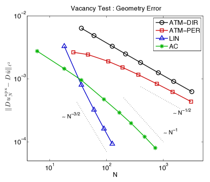
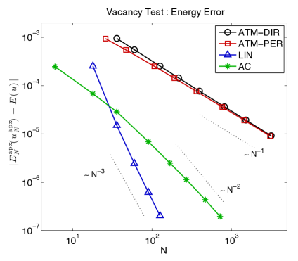
(a)                                                                             (b)

Figure 2. Rates of convergence, in the vacancy example, of four types of boundary conditions for (a) the geometry error and (b) the energy error. $N$ denotes the number of atoms in the inner computational domain; see § 2.7.1 for definitions.

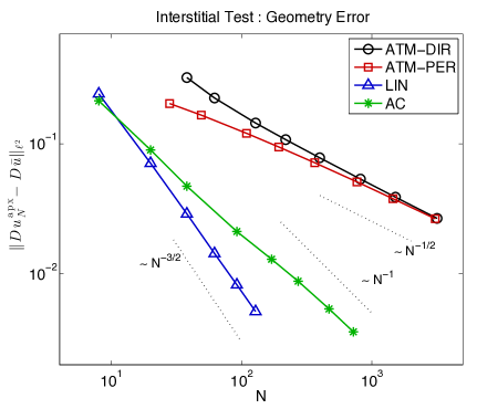
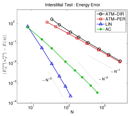
(a)                                                                             (b)

Figure 3. Rates of convergence, in the interstitial example, of four types of boundary conditions for (a) the geometry error and (b) the energy error; see § 2.7.1 for definitions.

3. Dislocations

We now present an atomistic model for dislocations and analogous regularity and approximation results. To avoid excessive duplication we will occasionally build on and reference § 2. Our presentation also builds on the descriptions in [2, 18]. For more general introductions to dislocations, including modeling aspects as well as analytical and computational solution strategies we refer to [7, 17].

3.1. Atomistic model

We consider a model for straight dislocation lines obtained by projecting a 3D crystal. Briefly, let ${\sf B}\mathbb{Z}^{3}$ denote a 3D Bravais lattice, oriented in such a way that the dislocation direction can be chosen parallel to $e_{3}$ and the Burgers vector can be chosen as ${\sf b}=({\sf b}_{1},0,{\sf b}_{3})\in{\sf B}\mathbb{Z}^{3}$. We consider displacements $W:{\sf B}\mathbb{Z}^{3}\to\mathbb{R}^{3}$ of the 3D lattice that are independent of the direction of the dislocation direction, i.e., $e_{3}$. Thus, we choose a projected reference lattice $\Lambda:={\sf A}\mathbb{Z}^{2}:=\{(\ell_{1},\ell_{2})\,|\,\ell\in{\sf B}\mathbb{Z}^{3}\}$, and identify $W(X)=w(X_{12})$, where $w:\Lambda\to\mathbb{R}^{3}$, and here and throughout we write $a_{12}=(a_{1},a_{2})$ for a vector $a\in\mathbb{R}^{3}$. It can be readily checked that this projection is again a Bravais lattice.

We may again choose a regular triangulation $\mathcal{T}_{\Lambda}$ satisfying $\mathcal{T}_{\Lambda}+\rho=\mathcal{T}_{\Lambda}$ for all $\rho\in\Lambda$. Each lattice function $v:\Lambda\to\mathbb{R}^{m}$ has an associated P1 interpolant $Iv:\mathbb{R}^{2}\to\mathbb{R}^{m}$ and we identify $\nabla v=\nabla Iv$. Further, we recall the definition of the spaces $\dot{\mathscr{W}}^{\rm c},\dot{\mathscr{W}}^{1,2}$ from (2.1).

Let $\hat{x}\in\mathbb{R}^{2}$ be the position of the dislocation core and $\Gamma:=\{x\in\mathbb{R}^{2}\,|\,x_{2}=\hat{x}_{2},x_{1}\geq\hat{x}_{1}\}$ the “branch-cut” (cf. (3.3)), chosen such that $\Gamma\cap\Lambda=\emptyset$. In order to model dislocations the site energy potential must be invariant under lattice slip. Normally, this is a consequence of permutation invariance of the site energy, but here we will formulate a minimal assumption. To that end, we define the slip operator $S_{0}$ acting on a displacement $w:\Lambda\to\mathbb{R}^{3}$, or $w:\mathbb{R}^{2}\to\mathbb{R}^{3}$, by

$$S_{0}w(x):=\left\{\begin{array}[]{rl}w(x),&x_{2}>\hat{x}_{2},\\ w(x-{\sf b}_{12})-{\sf b},&x_{2}<\hat{x}_{2}.\end{array}\right.$$ (3.1)

This operation leaves the 3D atom configuration corresponding to the displacement $u$ invariant: if $Y(X)=X+w(X_{12})$ and $Y^{S}(X)=X+S_{0}w(X_{12})$, then $Y(X)=Y^{S}(X)$ for $X_{2}>\hat{x}_{2}$, while for $X_{2}<\hat{x}_{2}$,

$$Y^{S}(X)=X+w(X_{12}-{\sf b}_{12})-{\sf b}=[X-{\sf b}]+w([X-{\sf b}]_{12})=Y(X-{\sf b}),$$

that is, $Y^{S}$ represents only a relabelling of the atoms. Therefore, formally, if $V(Dw)$ is the site energy potential as a function of displacement, then it must by invariant under the map $w\mapsto S_{0}w$:

$$\left\{\begin{array}[]{rl}V(DS_{0}w(\ell))=V(Dw(\ell)),&\text{ for $\ell_{2}>\hat{x}_{2}$},\\ V(DS_{0}w(\ell+{\sf b}_{12}))=V(Dw(\ell)),&\text{ for $\ell_{2}<\hat{x}_{2}$.}\end{array}\right.$$ (3.2)

In (3.6) below we will restate this assumption for a restricted class of displacements only, which will allow us to continue to employ the finite range interaction assumption.

Dislocations in an infinite lattice store infinite energy due to their topological singularity. We therefore decompose the total displacement $w=u_{0}+\bar{u}$ into a far-field predictor $u_{0}$ and a finite energy core corrector $\bar{u}$, where the latter belongs again to the energy space $\dot{\mathscr{W}}^{1,2}$. There is no unique way to specify $u_{0}$, but a natural choice is the continuum elasticity solution: For a function $u:\mathbb{R}^{2}\setminus\Gamma\to\mathbb{R}^{m}$ that has traces from above and below, we denote these traces, respectively, by $u(x\pm),x\in\Gamma$. Then we seek $u^{\rm lin}\in C^{\infty}(\mathbb{R}^{2}\setminus\Gamma;\mathbb{R}^{3})$ satisfying

$$\begin{split}\mathbb{C}_{i\alpha}^{j\beta}\frac{\partial^{2}u^{\rm lin}_{i}}{\partial x_{\alpha}\partial x_{\beta}}&=0\qquad\text{ in }\mathbb{R}^{2}\setminus\Gamma,\\ u^{\rm lin}(x+)-u^{\rm lin}(x-)&=-{\sf b}\qquad\text{ for }x\in\Gamma\setminus\{\hat{x}\},\\ \nabla_{e_{2}}u^{\rm lin}(x+)-\nabla_{e_{2}}u^{\rm lin}(x-)&=0\qquad\text{ for }x\in\Gamma\setminus\{\hat{x}\},\end{split}$$ (3.3)

where the tensor $\mathbb{C}$ is the linearised Cauchy–Born tensor (derived from the interaction potential $V$; see § A.2 for more detail).

In our analysis we require that applying the slip operator to the predictor map $u_{0}$ yields a smooth function in the half-space

$$\Omega_{\Gamma}:=\{x_{1}\geq\hat{x}_{1}\}\setminus B_{\hat{r}+{\sf b}_{1}}(\hat{x})$$ (3.4)

where $\hat{r}$ is defined in Lemma 3.1 below. That is, we require that $S_{0}u_{0}\in C^{\infty}(\Omega_{\Gamma})$. Except in the pure screw dislocation case (${\sf b}_{12}=0$) $u^{\rm lin}$ does not satisfy this property. The origin of this conundrum is that linearised elasticity assumes infinitesimal displacements, yet we apply it in the large deformation regime near the defect core. To overcome this technical difficulty, instead of $u_{0}=u^{\rm lin}$, we define the predictor

$$u_{0}(x):=u^{\rm lin}(\xi^{-1}(x)),\qquad\text{where}\qquad\xi(x):=x-{\sf b}_{12}{\textstyle\frac{1}{2\pi}}\eta(|x-\hat{x}|/\hat{r})\arg(x-\hat{x}),$$ (3.5)

$\arg(x)$ denotes the angle in $(0,2\pi)$ between ${\sf b}_{12}\propto e_{1}$ and $x$, and $\eta\in C^{\infty}(\mathbb{R})$ with $\eta=0$ in $(-\infty,0]$, $\eta=1$ in $[1,\infty)$ and $\eta^{\prime}>0$ in $(0,1)$. While the distinction between $u_{0}$ and $u^{\rm lin}$ is crucial, it arises from a subtle technical issue and could be ignored on a first reading, especially in view of the following lemma.

Lemma 3.1. (i) Suppose that the lattice is stable (2.7), then $u^{\rm lin}$ is well-defined. For $\hat{r}$ sufficiently large, $\xi:\mathbb{R}^{2}\setminus\Gamma\to\mathbb{R}^{2}\setminus\Gamma$ is a bijection, hence $u_{0}$ is also well-defined on $\mathbb{R}^{2}\setminus\Gamma$.

(ii) We have $\nabla^{j}S_{0}u_{0}(x+)=\nabla^{j}S_{0}u_{0}(x-)$ for all $j\geq 0$ and for all $x\in\Gamma\cap\Omega_{\Gamma}$. In particular, upon extending $u_{0}$ continuously to $\Gamma\cap\Omega_{\Gamma}$ we obtain that $S_{0}u_{0}\in C^{\infty}(\Omega_{\Gamma})$.

(iii) There exists $C$ such that $|\nabla^{n}u_{0}(x)-\nabla^{n}u^{\rm lin}(\xi^{-1}(x))|\leq C|x|^{-n-1}$ for $x\in\mathbb{R}^{2}\setminus(\Gamma\cup B_{r})$; in particular $|\nabla^{n}u_{0}(x)|\leq C|x|^{-n}$ for all $n\in\mathbb{N}$.

Proof.

The proof is given in § 5.3. ∎

Statement (ii) implies that the net-Burgers vector of $u_{0}$ (and hence of any $u_{0}+u,u\in\dot{\mathscr{W}}^{1,2}$) is indeed ${\sf b}$. Moreover, the fact that $S_{0}u_{0}\in C^{\infty}(\Omega_{\Gamma})$ will allow us to perform Taylor expansions of finite differences.Statement (iii) indicates that $u_{0}$ is an approximate far-field equilibrium, which allows us to use $u_{0}$ as a far-field boundary condition (see Lemma 3.1 below).

In order to keep the analysis as simple as possible we would like to keep the convenient assumption made in the point defect case of a finite interaction range in reference configuration. At first glance this contradicts the invariance of the site energy under lattice slip (3.1), but we can circumvent this by restricting the admissible corrector displacements. Arguing as in § B.1 we may choose sufficiently large radii $\hat{r}_{\mathscr{A}},\hat{m}_{\mathscr{A}}$ and define

$$\mathscr{A}:=\big{\{}u:\Lambda\to\mathbb{R}^{3}\,\big{|}\,\|\nabla u\|_{L^{\infty}}<\hat{m}_{\mathscr{A}}\text{ and }|\nabla u(x)|<1/2\text{ for }|x|>\hat{r}_{\mathscr{A}}\big{\}}.$$

Upon choosing $\hat{m}_{\mathscr{A}},\hat{r}_{\mathscr{A}}$ sufficiently large, we can ensure that any potential equilibrium solution is contained in $\mathscr{A}$. Thus, the restriction of admissible displacements to $\mathscr{A}$ is purely an analytical tool, which ensures that we can treat $V$ as having finite range, despite admitting slip-invariance.

For $w=u_{0}+u,u\in\mathscr{A}$, we shall write $S_{0}w=S_{0}u_{0}+Su$, where $S$ is an $\ell^{2}$-orthogonal operator, with dual $R=S^{*}=S^{-1}$,

$$Su(\ell):=\left\{\begin{array}[]{rl}u(\ell),&\ell_{2}>\hat{x}_{2},\\ u(\ell-{\sf b}_{12}),&\ell_{2}<\hat{x}_{2}\end{array}\right.\quad\text{and}\quad Ru(\ell):=\left\{\begin{array}[]{rl}u(\ell),&\ell_{2}>\hat{x}_{2},\\ u(\ell+{\sf b}_{12}),&\ell_{2}<\hat{x}_{2}.\end{array}\right.$$

We can now rigorously formulate the assumptions on the site energy potential: We assume that $V\in C^{k}((\mathbb{R}^{3})^{\mathcal{R}})$, $k\geq 4$, where $\mathcal{R}\subset\Lambda\setminus\{0\}$ such that for each $u\in\mathscr{A}$, and $w=u_{0}+u$, the site energy associated with a lattice site $\ell$ is given by $V(Dw(\ell))$, where $Dw(\ell)\equiv D_{\mathcal{R}}w(\ell)$. We assume again that $V({\bm{0}})=0$ (that is, $V$ is the energy difference from the reference lattice) and that $\mathcal{R},V$ are point symmetric (2.3). We shall assume throughout that $V$ is invariant under lattice slip, reformulating (3.2) as

$$V\big{(}D(u_{0}+u)(\ell)\big{)}=V\big{(}RDS_{0}(u_{0}+u)(\ell)\big{)}\qquad\forall u\in\mathscr{A},\ell\in\Lambda.$$ (3.6)

In addition, to guarantee lattice stability (both before and after shift) we assume that not only $D$ but also $RDS$ include nearest-neighbour finite differences (or equivalent):

$$|u(\ell+{\sf A}e_{n})-u(\ell)|\leq|RDSu(\ell)|,\qquad\forall\,\ell\in\Lambda,\quad n\in\{1,2\},\quad u:\Lambda\to\mathbb{R}^{3}.$$ (3.7)

The global energy (difference) functional is now defined by

$$\mathscr{E}(u):=\sum_{\ell\in\Lambda}\Big{(}V\big{(}Du_{0}(\ell)+Du(\ell)\big{)}-V\big{(}Du_{0}(\ell)\big{)}\Big{)}=:\sum_{\ell\in\Lambda}V_{\ell}(Du(\ell)),$$ (3.8)

where $V_{\ell}({\bm{g}}):=V(Du_{0}(\ell)+{\bm{g}})-V(Du_{0}(\ell))$.

Lemma 3.2. $\mathscr{E}:(\dot{\mathscr{W}}^{\rm c}\cap\mathscr{A},\|\nabla\cdot\|_{L^{2}})\to\mathbb{R}$ is continuous. In particular, there exists a unique continuous extension of $\mathscr{E}$ to $\mathscr{A}$, which we still denote by $\mathscr{E}$. The extended functional $\mathscr{E}\in C^{k}(\mathscr{A})$ in the sense of Fréchet.

Idea of the proof.

The main idea is the same as in the point defect case. The proof that $\delta\mathscr{E}(0)\in\dot{\mathscr{W}}^{-1,2}$ is based on the construction of $u_{0}$ in terms of the linear elasticity predictor $u^{\rm lin}$, which guarantees that $u_{0}$ is an “approximate equilibrium” in the far-field. See [19] for a similar proof applied in the simplified context of a screw dislocation. The complete proof (given in § 5.4) for our general case requires a combination of the proof in [19] and the concept of elastic strain introduced in § 3.2. ∎

The variational problem for the dislocation case is

$$\bar{u}\in\arg\min\big{\{}\mathscr{E}(u)\,\big{|}\,u\in\mathscr{A}\big{\}}.$$ (3.9)

Since $\mathscr{A}$ is open, if a minimiser $\bar{u}$ exists, then $\delta\mathscr{E}(\bar{u})=0$. We call a minimiser strongly stable if, in addition, it satisfies the positivity assumption (2.6).

Remark 3.3. One can also formulate anti-plane models for pure screw dislocations by restricting $\mathscr{A}$ to displacements of the form $u=(0,0,u_{3})$ and also computing a predictor of the form $u^{\rm lin}=(0,0,(u^{\rm lin})_{3})$. Note also that for pure screw dislocations, (3.5) is ignored. In the anti-plane case we may also choose $\mathscr{A}=\dot{\mathscr{W}}^{1,2}$ since only slip-invariance in anti-plane direction is required, that is, the topology of the projected 2D lattice remains unchanged.

To define in-plane models for pure edge dislocations one restricts $\mathscr{A}$ to displacements of the form $u=(u_{1},u_{2},0)$. The predictor $u^{\rm lin}$ does not simplify in this case.

All our results carry over trivially to these simplified models. ∎

Remark 3.4. The definition of the reference solution with branch-cut $\Gamma=\{(x_{1},\hat{x}_{2})\,|\,x_{1}\geq\hat{x}_{1}\}$ was somewhat arbitrary, in that we could have equally chosen $\Gamma_{S}:=\{(x_{1},\hat{x}_{2})\,|\,x_{1}\leq\hat{x}_{1}\}$. In this case the predictor solution $u_{0}$ would be replaced with $S_{0}u_{0}$. Let the resulting energy functional be denoted by

$$\mathscr{E}_{S}(v):=\sum_{\ell\in\Lambda}V\big{(}DS_{0}u_{0}(\ell)+Dv(\ell)\big{)}-V\big{(}DS_{0}u_{0}(\ell)\big{)}.$$

It is straightforward to see that, if $\delta\mathscr{E}(\bar{u})=0$, then $\delta\mathscr{E}_{S}(S\bar{u})=0$ as well. This observation means, that in certain arguments, an estimate on $\bar{u}$ in the left half-space where no branch-cut is present immediately yields the corresponding estimate on $S\bar{u}$ in the right half-space as well. ∎

Remark 3.5. Another source of arbitrariness comes from the precise definition of the predictor $u_{0}$, e.g., through the choice of the dislocation core position $\hat{x}$ or the choice of smearing function $\eta$. Indeed, more generally, arbitrary smooth modifications to $u_{0}$ are allowed as long as they do not significantly change the far-field behaviour. While such changes to the predictor $u_{0}$ affect the resulting corrector $\bar{u}$ (the solution of (3.9), the total displacement $u_{0}+\bar{u}$ remains unchanged in the sense that, if $u_{0}^{\prime}=u_{0}+w_{0}$ is a modified predictor, then $\bar{u}^{\prime}=\bar{u}-w_{0}$ is again a solution of (3.9). ∎

3.2. Elastic strain

The transformation $u_{0}\mapsto S_{0}u_{0}$ produces a map that is smooth in $\Omega_{\Gamma}$, and which generates the same atomistic configuration. It is therefore natural to define the elastic strains

$$e(\ell):=(e_{\rho}(\ell))_{\rho\in\mathcal{R}}\quad\text{where}\quad e_{\rho}(\ell):=\left\{\begin{array}[]{rl}RD_{\rho}S_{0}u_{0}(\ell),&\ell\in\Omega_{\Gamma},\\ D_{\rho}u_{0}(\ell),&\text{otherwise.}\end{array}\right.$$ (3.10)

The analogous definition for the corrector displacement $u$ is

$$\tilde{D}u(\ell):=(\tilde{D}_{\rho}u(\ell))_{\rho\in\mathcal{R}}\quad\text{where}\quad\tilde{D}_{\rho}u(\ell):=\left\{\begin{array}[]{rl}RD_{\rho}Su(\ell),&\ell\in\Omega_{\Gamma},\\ D_{\rho}u(\ell),&\text{otherwise.}\end{array}\right.$$ (3.11)

The slip invariance condition (3.6) can now be rewritten as

$$V\big{(}D(u_{0}+u)(\ell)\big{)}=V\big{(}e(\ell)+\tilde{D}u(\ell)\big{)}\qquad\forall u\in\mathscr{A},\ell\in\Lambda.$$ (3.12)

Linearity of $S$ and hence of $\tilde{D}$ implies

$$\big{\langle}\delta V(D(u_{0}+u)),Dv\big{\rangle} =\big{\langle}\delta V(e+\tilde{D}u),\tilde{D}v\big{\rangle},$$ (3.13)

$$\big{\langle}\delta^{2}V(D(u_{0}+u))Dv,Dw\big{\rangle} =\big{\langle}\delta^{2}V(e+\tilde{D}u)\tilde{D}v,\tilde{D}w\big{\rangle},$$ (3.14)

and so forth.

3.3. Regularity

The regularity of the predictor $u_{0}$ is already stated in Lemma 3.1. We now state the regularity of the corrector $\bar{u}$. It is interesting to note that the regularity of the dislocation corrector $\bar{u}$ is, up to log factors, identical to the regularity of the displacement field in the point defect case, which indicates that the dislocation problem is computationally no more demanding than the point defect problem. Indeed, this will be confirmed in § 3.4.

Theorem 3.6. Suppose that the lattice is stable (2.7). Let $u\in\mathscr{A}$ be a critical point, $\delta\mathscr{E}(u)=0$, then there exist constants $C>0,u_{\infty}\in\mathbb{R}^{3}$ such that, for $1\leq j\leq k-2$ and for $|\ell|$ sufficiently large,

$$|\tilde{D}^{j}u(\ell)|\leq C|\ell|^{-1-j}\log|\ell|\qquad\text{and}\qquad|u(\ell)-u_{\infty}|\leq C|\ell|^{-1}\log|\ell|.$$ (3.15)

Remark 3.7. It can be immediately seen that the decay $|\tilde{D}u(\ell)|\lesssim|\ell|^{-2}\log|\ell|$ is equivalent to $|Du(\ell)|\lesssim|\ell|^{-2}\log|\ell|$. For higher-order derivatives, it is necessary to make a case distinction. While, $\tilde{D}^{j}u(\ell)=D^{j}u(\ell)$ at sufficient distance from $\Gamma$, “close to” the branchcut $\Gamma$ we could alternatively write $|D^{j}Su(\ell)|\lesssim|\ell|^{-1-j}$.

In the pure screw case where ${\sf b}_{12}=0$ we simply have $D=\tilde{D}$. ∎

3.4. Clamped boundary conditions

To extend clamped boundary conditions to the dislocation problem, we prescribe the displacement to be the predictor displacement outside some finite computational domain $\Omega_{R}\subset\Lambda$. Thus, we may think of these boundary conditions as asynchronous continuum linearised elasticity boundary conditions.

This amounts to choosing a corrector displacement space analogous to $\dot{\mathscr{W}}^{0}(\Omega_{R})$ in the point defect case,

$$\mathscr{A}^{0}(\Omega_{R}):=\big{\{}v\in\mathscr{A}\,\big{|}\,v=0\text{ in }\Lambda\setminus\Omega_{R}\big{\}},$$

and the associated finite-dimensional optimisation problem reads

$$u^{0}_{R}\in\arg\min\big{\{}\mathscr{E}(u)\,\big{|}\,u\in\mathscr{A}^{0}(\Omega_{R})\big{\}}.$$ (3.16)

Theorem 3.8. Let $\bar{u}$ be a strongly stable solution to (3.9), then there exist $C,R_{0}>0$ such that, for all $\Omega_{R}\subset\Lambda$ satisfying $B_{R}\cap\Lambda\subset\Omega_{R}$ for some $R\geq R_{0}$, there exists a strongly stable solution $\bar{u}^{0}_{R}$ of (3.16) satisfying

$$\|\nabla\bar{u}-\nabla\bar{u}^{0}_{R}\|_{L^{2}}\leq CR^{-1}\log(R)\qquad\text{and}\qquad\big{|}\mathscr{E}(\bar{u})-\mathscr{E}(\bar{u}^{0}_{R})\big{|}\leq CR^{-2}(\log R)^{2}.$$ (3.17)

3.5. Periodic boundary conditions

It is possible to extend periodic boundary conditions to the dislocation case by considering a periodic array of dislocations with alternating signs. In practise the computational domain then contains a dipole or a quadrupole. It then becomes necessary to estimate image effects, for which our regularity results are still useful, but which requires substantial additional work. Hence, we postpone the analysis of periodic boundary conditions for dislocation to future work, but refer to [8] for an interesting discussion of these issues.

3.6. Boundary conditions from linear elasticity

We now extend the lattice linear elasticity boundary conditions to the dislocation case. The linearisation argument (2.16) should now be carried out for the full displacement $w=u_{0}+u$, and reads

$$V(Dw)\approx V(0)+\langle\delta V(0),Dw\rangle+{\textstyle\frac{1}{2}}\langle\delta^{2}V(0)Dw,Dw\rangle,$$

but this is invalid whenever the interaction neighbourhood crosses the slip plane $\Gamma$.

Instead, we must first transform the finite difference stencils as follows: recall the definition of $\Omega_{\Gamma}$ from (3.4) and the definition of elastic strain $e$ and $\tilde{D}u$ from (3.10) and (3.11), then we define

$$\tilde{D}_{0}w(\ell)=\tilde{D}_{0}(u_{0}+u)(\ell):=e(\ell)+\tilde{D}u(\ell).$$ (3.18)

According to Lemma 3.1 and Theorem 3.3, if $u=\bar{u}$, then $|\tilde{D}_{0}w(\ell)|=O(|\ell|^{-1})$, hence we may linearize with respect to this transformed finite different stencil. Using the slip invariance condition (3.6), we obtain

$$V(Dw)=V(\tilde{D}_{0}w)=V(0)+\langle\delta V(0),\tilde{D}_{0}w\rangle+{\textstyle\frac{1}{2}}\langle\delta^{2}V(0)\tilde{D}_{0}w,\tilde{D}_{0}w\rangle+O(|\tilde{D}_{0}w|^{3}),$$

and we therefore define the energy difference functional

$$\mathscr{E}^{\rm lin}_{R}(u) :=\sum_{\ell\in\Omega_{R}}V_{\ell}(Du(\ell))+\sum_{\ell\in\Lambda\setminus\Omega_{R}}\Big{(}V^{\rm lin}\big{(}e(\ell)+\tilde{D}u(\ell)\big{)}-V^{\rm lin}\big{(}e(\ell)\big{)}\Big{)},$$

where $V^{\rm lin}$ is the same as in the point defect case,

$$V^{\rm lin}({\bm{g}}) :=V({\bm{0}})+\big{\langle}\delta V({\bm{0}}),{\bm{g}}\big{\rangle}+{\textstyle\frac{1}{2}}\big{\langle}\delta^{2}V({\bm{0}}){\bm{g}},{\bm{g}}\big{\rangle}$$

and where $\Omega_{R}\subset\Lambda$ is the “inner” computational domain. It follows from minor modifications of the proof of Lemma 3.1 that $\mathscr{E}^{\rm lin}_{R}$ can be extended by continuity to a functional $\mathscr{E}^{\rm lin}_{R}\in C^{k}(\mathscr{A})$.

Thus, we aim to compute

$$u^{\rm lin}_{R}\in\arg\min\big{\{}\mathscr{E}^{\rm lin}_{R}(u)\,\big{|}\,u\in\mathscr{A}\big{\}}.$$ (3.19)

Theorem 3.9. Let $\bar{u}$ be a strongly stable solution to (3.9), then there exist $C,R_{0}>0$ such that for all domains $\Omega_{R}\subset\Lambda$ with $B_{R}\cap\Lambda\subset\Omega_{R}$ and $R\geq R_{0}$, there exists a strongly stable solution of (3.19) satisfying

$$\big{\|}\nabla\bar{u}-\nabla u^{\rm lin}_{R}\big{\|}_{L^{2}}\leq CR^{-1}\qquad\text{and}\qquad\big{|}\mathscr{E}^{\rm lin}_{R}(u^{\rm lin}_{R})-\mathscr{E}(\bar{u})\big{|}\leq CR^{-2}\log R.$$ (3.20)

Idea of proof.

The proof is similar to the point defect case, the main additional step to take into account being that the linearisation is with respect to the full displacement $u_{0}+\bar{u}$. Since $\nabla u_{0}\sim|x|^{-1}$ it therefore follows that the linearisation error at site $\ell$ is only of order $O(|\ell|^{-2})$, while in the point defect case it was of order $O(|\ell|^{-2d})$. This accounts for the reduced convergence rate. ∎

Remark 3.10. 1. The key difference between the schemes (3.16) and (3.19) is that the former employs a precomputed continuum linear elasticity boundary condition while the latter computes a lattice linear elasticity boundary condition on the fly. It is therefore interesting to note that, for dislocations, solving the relatively complex exterior problem yields almost no qualitative improvement over the basic Dirichlet scheme (3.16). Indeed, if the cost of solving the exterior problem is taken into account as well, then the scheme (3.19) may in practice become more expensive than (3.16).

The main advantage of (3.19) appears to be that the boundary condition need not be computed beforehand, but could be computed “on the fly”. We speculate that this can give a substantially improved prefactor when the dislocation core is spread out, e.g., in the case of partials.

2. If, instead of linearising about the homogeneous lattice configuration we were to linearise about the predictor $u_{0}$, then the rate of convergence for dislocations would become the same (up to log factors) as for point defects. However, since lattice Green’s function and similar techniques are no longer available we cannot conceive of an efficient implementation of such a scheme without reverting again to complex atomistic/continuum type coarse-graining techniques. ∎

3.7. Boundary conditions from nonlinear elasticity for screw dislocations

The formulation of a/c coupling methods for general dislocations is not straightforward. We therefore consider only the case of pure screw dislocations and postpone the general case to future work. Thus, we assume that ${\sf b}=e_{3}$, and in this case, only the invariance of $V$ in the normal direction is relevant:

$$V\big{(}{\bm{g}}+{\bm{h}}e_{3}\big{)}=V({\bm{g}})\qquad\forall{\bm{g}}\in(\mathbb{R}^{3})^{\mathcal{R}},{\bm{h}}\in\mathbb{Z}^{\mathcal{R}}.$$

We set up the computational domain and approximation space as in § 2.6. To define the energy functional, we first construct a modified interpolant that takes into account the discontinuity of the full displacement across the slip plane, similarly to the elastic strain used in § 3.6,

$$I_{R}^{\rm el}u(x):=\left\{\begin{array}[]{rl}I_{R}u(x),&x\in T,T\cap\Gamma=\emptyset,\\ I_{R}(u+{\sf b}\chi_{x_{2}<\hat{x}_{2}})(x),&x\in T,T\cap\Gamma\neq\emptyset,\end{array}\right.,$$

where $I_{R}$ is the nodal interpolation with respect to $\mathcal{T}_{R}$. With this definition, the energy difference functional is given by

$$\mathscr{E}^{\rm ac}_{R}(u) :=\sum_{\ell\in\Omega^{\rm a}_{R}}V_{\ell}(Du(\ell))+\sum_{\ell\in\Omega^{\rm i}_{R}}V_{\ell}^{\rm i}(Du(\ell))$$ (3.21)

$$\qquad\qquad+\sum_{T\in\mathcal{T}_{R}}v_{T}^{\rm eff}\Big{(}W(\nabla I^{\rm el}_{R}(u_{0}+u))-W(\nabla I^{\rm el}_{R}u_{0})\Big{)},$$

where $V_{\ell}^{\rm i},W,v_{T}^{\rm eff}$ are defined as in § 2.6.

We seek to compute

$$u^{\rm ac}_{R}\in\arg\min\big{\{}\mathscr{E}^{\rm ac}_{R}(u)\,\big{|}\,u\in\mathscr{A}(\mathcal{T}_{R})\big{\}},\qquad\text{where}$$ (3.22)

$$\mathscr{A}(\mathcal{T}_{R}):=\mathscr{A}\cap\dot{\mathscr{W}}^{0}(\mathcal{T}_{R}).$$

We again let $R$ and $R_{\rm c}$ be the sizes of $\Omega^{\rm a}_{R}$ and $\omega_{R}$,

$$B_{R}\cap\Lambda\subset\Omega^{\rm a}_{R}\qquad\text{and}\qquad B_{R_{\rm c}}\subset\omega_{R}\subset B_{c_{0}R_{\rm c}}.$$ (3.23)

and assume that there exists $\eta>0$ and $c_{1}>0$ such that there exists a strongly stable solution $\bar{u}^{\rm ac}_{R}$ to (3.22) satisfying

$$\|\nabla\bar{u}^{\rm ac}_{R}-\nabla\bar{u}\|\leq c_{1}\big{(}\|h\tilde{D}^{2}(u_{0}+\bar{u})\|_{\ell^{2}(\Lambda\cap(\omega_{R}\setminus B_{R}))}+\|\tilde{D}\bar{u}\|_{\ell^{2}(\Lambda\setminus B_{R_{\rm c}/2})}\big{)},$$ (3.24)

provided that $\|h\tilde{D}^{2}(u_{0}+\bar{u})\|_{\ell^{2}(\Lambda\cap(\omega_{R}\setminus B_{R}))}+\|\tilde{D}\bar{u}\|_{\ell^{2}(\Lambda\setminus B_{R_{\rm c}/2})}\leq\eta$.

Proposition 3.11. Let $\bar{u}$ be a strongly stable solution of (3.9) and assume that (3.23) and (3.24) hold. Further we require that $\omega_{R}$ and $\mathcal{T}_{R}$ satisfy the following quasi-optimality conditions:

$$c_{2}R^{p}\leq R_{\rm c}\leq c_{3}R^{p},\text{ for some $p>0$, \qquad and}\qquad|h(x)|\leq c_{4}{\textstyle\frac{|x|}{R}}.$$ (3.25)

Then there exist $R_{0},C$ depending on $\eta$, $c_{2}$, $c_{3}$, $c_{4}$, and $p$, such that for all $R\geq R_{0}$ there exists a strongly stable solution $\bar{u}^{\rm ac}_{R}$ to (3.22) satisfying

$$\big{\|}\nabla\bar{u}^{\rm ac}_{R}-\nabla\bar{u}\big{\|}_{L^{2}} \leq CR^{-1}.$$ (3.26)

3.8. Numerical results

3.8.1. Setup

We consider the anti-plane deformation model of a screw dislocation in a BCC crystal from [19], the main difference being that we admit nearest neighbour many-body interactions instead of only pair interactions. Thus, we only give a brief outline of the model setup. The choice of dislocation type is motivated by the fact that the linearised elasticity solution is readily available.

Briefly, let ${\sf B}\mathbb{Z}^{3}=\mathbb{Z}^{3}\cup(\mathbb{Z}^{3}+(1/2,1/2,1/2)^{T})$ denote a BCC crystal, then both the dislocation core and Burgers vector point in the $(1,1,1)^{T}$ direction. Upon rotating and possibly dilating, the projection ${\sf A}\mathbb{Z}^{2}$ of the BCC crystal is a triangular lattice, hence we again assume (2.25). The linear elasticity predictor is now given by $u^{\rm lin}(x)={\textstyle\frac{1}{2\pi}}{\rm arg}(x-\hat{x})$, where we assumed that the Burgers vector is $b=(0,0,1)^{T}$ and $\hat{x}$ is the centre of the dislocation core. We shall slightly generalise this, by admitting

$$u^{\rm lin}(x)={\sf F}\cdot(x-\hat{x})+{\textstyle\frac{1}{2\pi}}{\rm arg}(x-\hat{x}),$$

which is equivalent to applying a shear deformation of the form

$$\left(\begin{array}[]{ccc}1&0&0\\ 0&1&0\\ {\sf F}_{1}&{\sf F}_{2}&1\end{array}\right)$$

to the rotated BCC crystal and is thus still included within our framework through a modification of the potential $V$.

Let the unknown for the anti-plane model, the displacement in $e_{3}$ direction, be denoted by $z(\ell):=y_{3}(\ell)$, then we use the EAM-type site potential

$$V(Dy(\ell))=V^{\rm anti}(Dz(\ell))=\sum_{\rho\in\mathcal{N}_{\ell}}\phi\big{(}|D_{\rho}z(\ell)|\big{)}+G\Big{(}\sum_{\rho\in\mathcal{N}_{\ell}}\psi\big{(}|D_{\rho}z(\ell)|\big{)}\Big{)}$$

$$\text{with }\phi(r)=\psi(r)=\sin^{2}(\pi r)\quad\text{ and }G(s)={\textstyle\frac{1}{2}}s^{2}.$$

The $1$-periodicity of $\phi,\psi$ emulates the fact that displacing a line of atoms by a full Burgers vector leaves the energy invariant.

We apply again the remaining remarks in § 2.7.1.

3.8.2. Discussion of results

We consider three numerical experiments:

1. ${\sf F}=(0,0)^{T},x_{0}=(1/3,1/(2\sqrt{3}))^{T}$:
    The results are shown in Figure 5. We observe precisely the predicted rates of convergence. However, it is worth noting that although the asymptotic rates for ATM, LIN and AC are identical (up to log-factors), the prefactor varies by an order of magnitude.

   The “dip” in the energy error for the LIN method is likely due to a change in sign of the error.

2. ${\sf F}=(0,0)^{T},x_{0}={\textstyle\frac{1}{2}}(1,1/\sqrt{3})^{T}$ is the centre of a triangle:
    The results are shown in Figure 6. In this case, the AC method exhibits the predicted convergence rate, while both the ATM and LIN methods show subtantially better rates. The explanation for ATM (but not for LIN) is that the solution displacement $\bar{u}$ has three-fold symmetry, from which one can formally deduce the improved decay estimate $|D\bar{u}(\ell)|\leq C|\ell|^{-4}$. This readily implies the observed rate.

   This test demonstrates that, in general, our estimates are only upper bounds, but that in special circumstances (e.g., additional symmetries), better rates can be obtained. It is moreover interesting to note that the most basic scheme, ATM, is the most accurate with this setup.

3. ${\sf F}=(10^{-3},3\times 10^{-4})^{T},x_{0}={\textstyle\frac{1}{2}}(1,1/\sqrt{3})^{T}$:
    The results are shown in Figure 7. In this final test, we chose ${\sf F}$ to push the dislocation core close to instability. We included this test to demonstrate that one cannot always expect the clean convergence rates displayed in the point defect tests, or in the first screw dislocation test, but that there may be significant pre-asymptotic regimes.

Figure 4. Illustration of a screw dislocation configuration in a BCC crystal.

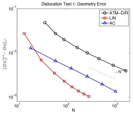
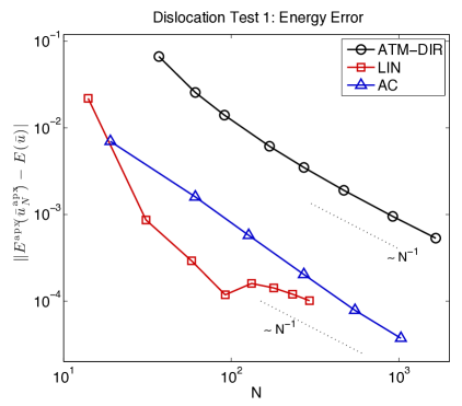
(a)                                                                             (b)

Figure 5. Rates of convergence, in the first dislocation test, of the ATM-DIR, LIN and AC methods. $N$ denotes the number of atoms in the inner computational domain; see § 2.7.1 for definitions.

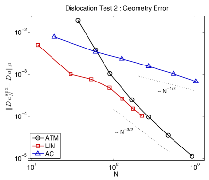
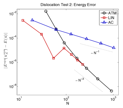
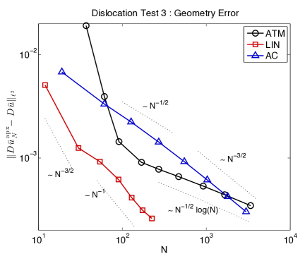
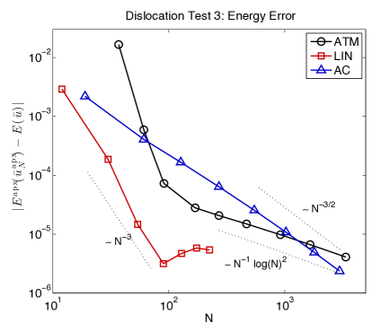
(a)                                                                             (b)

Figure 6. Rates of convergence, in the second dislocation test, of the ATM-DIR, LIN and AC methods. $N$ denotes the number of atoms in the inner computational domain; see § 2.7.1 for definitions.

(a)                                                                             (b)

Figure 7. Rates of convergence, in the third dislocation test, of the ATM-DIR, LIN and AC methods. $N$ denotes the number of atoms in the inner computational domain; see § 2.7.1 for definitions.

4. Conclusion

We have introduced a flexible analytical framework to study the effect of embedding a defect in an infinite crystalline environment. Our main analytical results are (1) the formulation of equilibration as a variational problem in a discrete energy space; and (2) a qualitatively sharp regularity theory for minimisers.

These results are generally useful for the analysis of crystalline defects, however, our own primary motivation was to provide a foundation for the analysis of atomistic multi-scale simulation methods, which in this context can be thought of as different means to produce boundary conditions for an atomistic defect core simulation. To demonstrate the applicability of our framework we analyzed simple variants of some of the most commonly employed schemes: Dirichlet boundary conditions, periodic boundary conditions, far-field approximation via linearised lattice elasticity and via nonlinear continuum elasticity (Cauchy–Born, atomistic-to-continuum coupling). In parallel works [35, 23, 22, 12] this framework has already been exploited resulting in new and improved formulations of atomistic/continuum and quantum/atomistic coupling schemes.

There are numerous practical and theoretical questions that we have left open in the present work, some of which we commented on throughout the article. Possibly the key “bottleneck” in our analysis is that it only provides a rate of convergence, i.e.,

$$\text{error}\leq CN^{-r},$$

where $N$ is the number of unknowns in the approximate problem, however, we have not been able to provide estimates on the prefactor. We speculate that such estimates may not be obtained a priori but only a posteriori, as it requires considerably more detailed information about a defects structure and stability than one would normally assume a priori.

5. Proofs: The Energy Difference Functionals

This section is concerned with proofs for Lemma 1 and Lemma 3.1 which state that the energy $\mathscr{E}$ can be understood as a smooth functional on the energy space, i.e., $\mathscr{E}\in C^{k}(\dot{\mathscr{W}}^{1,2})$ in the point defect case and $\mathscr{E}\in C^{k}(\mathscr{A})$ in the dislocation case.

5.1. Conversion to divergence form

We begin by establishing an auxiliary result that allows us to convert pointwise forces into divergence form without sacrificing fundamental decay properties.

Lemma 5.1. Let $d\in\mathbb{N}$, $p>d\geq 2$ and $f:\mathbb{Z}^{d}\to\mathbb{R}$ such that $|f(\ell)|\leq C_{f}|\ell|^{-p}$ for all $\ell\in\mathbb{Z}^{d}$. Suppose, in addition, that $\sum_{\ell\in\mathbb{Z}^{d}}f(\ell)=0$. Then, there exists $g:\mathbb{Z}^{d}\to\mathbb{R}^{d}$ and a constant $C$ depending only on $p$ and $d$ such that

$$\sum_{j=1}^{d}D_{e_{j}}g_{j}(\ell)=f(\ell)\quad\text{and}\quad|g(\ell)|\leq CC_{f}|\ell|^{-p+1}\quad\text{for all }\ell\in\mathbb{Z}^{d}.$$ (5.1)

If $f$ has compact support, then $g$ can be chosen to have compact support as well.

Proof.

Denote $\bar{\ell}:=(\ell_{1},\dots,\ell_{d-1})^{T}$. We define the operator $\mathcal{C}_{d}(f,g):=(\tilde{f},\tilde{g})$, where $\tilde{g}:=g+\Delta\tilde{g}\,e_{d}$,

$$\Delta\tilde{g}(\bar{\ell},\ell_{d}):=\left\{\begin{array}[]{rl}\sum_{\lambda=\ell_{d}}^{3\ell_{d}-2}f(\bar{\ell},\lambda),&\ell_{d}\geq 1,\\ -\sum_{\lambda=3\ell_{d}-1}^{\ell_{d}-1}f(\bar{\ell},\lambda),&\ell_{d}\leq 0,\end{array}\right.\quad\text{and}\quad\tilde{f}(\bar{\ell},\ell_{d}):=\sum_{\lambda=3\ell_{d}-1}^{3\ell_{d}+1}f(\bar{\ell},\lambda).$$

One can then readily verify that

$$D_{e_{d}}g_{d}(\ell)-f(\ell)=D_{e_{d}}\tilde{g}_{d}(\ell)-\tilde{f}(\ell)\qquad\forall\ell\in\mathbb{Z}^{d}.$$ (5.2)

Moreover it is easy to see from the definition that $\sum_{\ell\in\mathbb{Z}^{d}}\tilde{f}(\ell)=\sum_{\ell\in\mathbb{Z}^{d}}f(\ell)=0$.

Let the operators $\mathcal{C}_{1},\dots,\mathcal{C}_{d-1}$ be defined analogously and let $\mathcal{C}$ be their composition $\mathcal{C}:=\mathcal{C}_{1}\circ\dots\circ\mathcal{C}_{d}$. If $(f^{+},g^{+})=\mathcal{C}(f,g)$, then from (5.2) we obtain that

$$f^{+}(\ell)-\sum_{j=1}^{d}D_{e_{j}}g^{+}_{j}(\ell)=f(\ell)-\sum_{j=1}^{d}D_{e_{j}}g_{j}(\ell).$$ (5.3)

Define the seminorm $[f]_{q}:=\sup_{\ell\in\mathbb{Z}^{d}\setminus\{0\}}(|\ell|_{\infty}-{\textstyle\frac{1}{2}})^{q}|f(\ell)|$, and a norm $\llbracket g\rrbracket_{q}:=\sup_{\ell\in\mathbb{Z}^{d}}(|\ell|_{\infty}+{\textstyle\frac{1}{2}})^{q}|g(\ell)|$. We claim that, if $(f^{+},g^{+})=\mathcal{C}(f,g)$, then

$$[f^{+}]_{p}\leq 3^{d-p}[f]_{p}\quad\text{and}\quad\llbracket g^{+}-g\rrbracket_{p-1}\lesssim[f]_{p},$$ (5.4)

where $\lesssim$ denotes comparison up to a multiplicative constant that may only depend on $p$ and $d$. Suppose that we have established (5.4). We define

$$f^{(0)}:=f,\quad g^{(0)}:=0,\quad\text{and}\quad(f^{(n+1)},g^{(n+1)}):=\mathcal{C}(f^{(n)},g^{(n)})\quad\text{for all $n\in\mathbb{Z}_{+}$}.$$

Since $p>d$, we obtain that $[f^{(n)}]_{p}\to 0$. Moreover, since $\sum_{\ell\in\mathbb{Z}^{d}}f^{(n)}(\ell)=0$ for all $n$ it follows that $\|f^{(n)}\|_{\ell^{1}}\to 0$. Further, (5.4) implies

$$\llbracket g^{(n+1)}-g^{(n)}\rrbracket_{p-1}\lesssim[f^{(n)}]_{p}\leq 3^{n(d-p)}[f]_{p},$$

and hence the series $\sum_{n=0}^{\infty}g^{(n+1)}-g^{(n)}$ converges. Let $g(\ell):=\lim_{n\to\infty}g^{(n)}(\ell)$, then (5.3) implies that $g$ satisfies the identity in (5.1), and the bound on $\llbracket g\rrbracket_{p-1}$ implies the inequality in (5.1). It remains to note that if $f=f(\ell)=0$ outside the region $|\ell|_{\infty}\leq L$ for some $L$, then $f^{(n)}$, $g^{(n)}$, and hence $g$, are also zero outside this region.

To show the first inequality in (5.4), we fix $\ell\neq 0$, express $f^{+}(\ell)$ through $f(\ell)$, and estimate

$$|f^{+}(\ell)|=~{} \Bigg{|}\sum_{\begin{subarray}{c}\lambda\in\mathbb{Z}^{d}\\ |\lambda-3\ell|_{\infty}\leq 1\end{subarray}}f(\lambda)\Bigg{|}\leq~{}\sum_{\begin{subarray}{c}\lambda\in\mathbb{Z}^{d}\\ |\lambda-3\ell|_{\infty}\leq 1\end{subarray}}\big{(}|\lambda|_{\infty}-{\textstyle\frac{1}{2}}\big{)}^{-p}[f]_{p}$$

$$\leq~{} \sum_{\begin{subarray}{c}\lambda\in\mathbb{Z}^{d}\\ |\lambda-3\ell|_{\infty}\leq 1\end{subarray}}\big{(}|3\ell|_{\infty}-1-{\textstyle\frac{1}{2}}\big{)}^{-p}[f]_{p}=3^{d}\,3^{-p}\big{(}|\ell|_{\infty}-{\textstyle\frac{1}{2}}\big{)}^{-p}[f]_{p}.$$

The second inequality in (5.4) is based on the following two estimates:

$$|\tilde{f}(\ell)|\leq 3(|\ell|_{\infty}-{\textstyle\frac{1}{2}})^{-p}[f]_{p}\qquad\text{and}\qquad|\Delta\tilde{g}(\ell)|\lesssim(|\ell|_{\infty}+{\textstyle\frac{1}{2}})^{-p+1}[f]_{p},$$

where we denote again $(\tilde{f},\tilde{g}):=\mathcal{C}_{d}(f,g)$ and $\Delta\tilde{g}:=(\tilde{g}-g)\cdot e_{d}$. The first estimate follows from arguments similar to the above. The second estimate, for $\ell=(\bar{\ell},\ell_{d})$ with $\ell_{d}\leq 0$, is proved in the following calculation:

$$|\Delta\tilde{g}(\ell)|\leq~{} \sum_{\lambda=3\ell_{d}-1}^{\ell_{d}-1}|f(\bar{\ell},\lambda)|\leq~{}[f]_{p}\sum_{\lambda=3\ell_{d}-1}^{\ell_{d}-1}(|(\bar{\ell},\lambda)|_{\infty}-{\textstyle\frac{1}{2}})^{-p}$$

$$\leq~{} [f]_{p}\sum_{\lambda=3\ell_{d}-1}^{\ell_{d}-1}(|(\bar{\ell},\ell_{d}-1)|_{\infty}-{\textstyle\frac{1}{2}})^{-p}\leq~{}[f]_{p}|2\ell_{d}-1|\,({\textstyle\frac{1}{3}}(|(\bar{\ell},\ell_{d}-1)|_{\infty}+{\textstyle\frac{1}{2}}))^{-p}$$

$$\leq~{} [f]_{p}\,|2\ell_{d}+1|\,{\textstyle\frac{1}{3^{p}}}(|\ell|_{\infty}+{\textstyle\frac{1}{2}})^{-p}\leq~{}[f]_{p}\,{\textstyle\frac{2}{3^{p}}}(|\ell|_{\infty}+{\textstyle\frac{1}{2}})^{-p+1},$$

where we used that for $\ell_{d}\leq 0$, $|(\bar{\ell},\ell_{d}-1)|_{\infty}\geq 1$ and the fact that $x-{\textstyle\frac{1}{2}}\geq{\textstyle\frac{1}{3}}(x+{\textstyle\frac{1}{2}})$ for any $x\geq 1$. For $\ell_{d}>0$ this estimate is obtained in a similar way.

The analogous estimates hold for applications of $\mathcal{C}_{d-1},\dots,\mathcal{C}_{1}$ and combining these yields the second inequality in (5.4). ∎

Corollary 5.2. Let $p>d$ ($d\in\{2,3\}$), and $f:{\sf A}\mathbb{Z}^{d}\to\mathbb{R}$ such that $|f(\ell)|\leq C_{f}|\ell|^{-p}$ for all $\ell\in{\sf A}\mathbb{Z}^{d}$, and $\sum_{\ell\in{\sf A}\mathbb{Z}^{d}}f(\ell)=0$. Then under the assumptions of § 2.1, there exists $g:{\sf A}\mathbb{Z}^{d}\to\mathbb{R}^{\mathcal{R}}$ and a constant $C$ depending only on $p$ such that

$$\sum_{\ell\in{\sf A}\mathbb{Z}^{d}}f(\ell)v(\ell) =\sum_{\ell\in{\sf A}\mathbb{Z}^{d}}\langle g(\ell),Dv(\ell)\rangle\quad|g(\ell)|\leq CC_{f}|\ell|^{-p+1}\quad\text{for all }\ell\in{\sf A}\mathbb{Z}^{d}.$$

In addition, if $d=2$, under the assumptions of § 3.1, there exists $\tilde{g}:{\sf A}\mathbb{Z}^{2}\to\mathbb{R}^{\mathcal{R}}$ such that

$$\sum_{\ell\in{\sf A}\mathbb{Z}^{2}}f(\ell)v(\ell) =\sum_{\ell\in{\sf A}\mathbb{Z}^{2}}\langle\tilde{g}(\ell),\tilde{D}v(\ell)\rangle\quad|\tilde{g}(\ell)|\leq CC_{f}|\ell|^{-p+1}\quad\text{for all }\ell\in{\sf A}\mathbb{Z}^{2}.$$

If $f$ has compact support, then $g$ and $\tilde{g}$ can be chosen to have compact support as well.

Proof.

One only needs to notice that the assumptions that the operators $D$ and $\tilde{D}$ contain nearest-neighbor finite differences (cf. (2.4) and (3.7)) allow to use Lemma 5.1 to construct the needed $g$ and $\tilde{g}$. ∎

5.2. Proof of Lemma 1

The proof relies on two prerequisites.

Lemma 5.3. Under the conditions of Lemma 1,

$$\mathscr{F}(u):=\sum_{\ell\in\Lambda}\Big{(}V_{\ell}(Du(\ell))-\langle\delta V_{\ell}({\bm{0}}),Du(\ell)\rangle\Big{)}$$

is well-defined for any $u\in\dot{\mathscr{W}}^{1,2}$, and $\mathscr{F}\in C^{k}(\dot{\mathscr{W}}^{1,2})$.

Proof.

For a very similar argument that can be followed almost verbatim see [33], hence we only give a brief idea of the proof.

Since $|Du(\ell)|\in\ell^{2}(\Lambda)$ implies $|Du(\ell)|\in\ell^{\infty}$ and since $V_{\ell}\equiv V$ for $|\ell|\geq R_{0}$, we obtain that $\|\delta^{2}V_{\ell}(tDu(\ell))\|\leq C$, where $C$ is independent of $t\in[0,1]$, and $\ell$. It follows that

$$\big{|}V_{\ell}(Du(\ell))-\langle\delta V_{\ell}({\bm{0}}),Du(\ell)\rangle\big{|}\leq C_{u}|Du(\ell)|^{2},$$

where $C_{u}$ depends only on $\|\,|Du|\,\|_{\ell^{\infty}}$. In particular, $\ell\mapsto V_{\ell}(Du(\ell))-\langle\delta V_{\ell}({\bm{0}}),Du(\ell)\rangle\in\ell^{1}(\Lambda)$, and hence $\mathscr{F}(u)$ is well-defined.

Using similar lines of argument one can prove that $\mathscr{F}\in C^{k}(\mathscr{A})$. ∎

Lemma 5.4. Under the conditions of Lemma 1, $\delta\mathscr{E}(0)\in\dot{\mathscr{W}}^{-1,2}$.

Proof.

Let $v\in\dot{\mathscr{W}}^{\rm c}$, then we can write the first variation in the form

$$\langle\delta\mathscr{E}(0),v\rangle=\sum_{\ell\in\Lambda}\langle\delta V_{\ell}({\bm{0}}),Dv(\ell)\rangle=\sum_{\ell\in\Lambda}f(\ell)\cdot v(\ell).$$

where $f(\ell)$ is given in terms of the $V_{\ell,\rho}$; the precise form is unimportant. Point symmetry of the lattice implies that $f(\ell)=0$ for $|\ell|>{R_{\rm def}}+r_{\rm cut}$. Since $\mathscr{E}$ is translation invariant ($\mathscr{E}(u+c)=\mathscr{E}(u)$ for $c(\ell)=c\in\mathbb{R}$), it follows that $\sum_{\ell\in\Lambda}f(\ell)=0$. Therefore,

$$\big{|}\langle f,u\rangle\big{|}=\big{|}\langle f,u-u(0)\rangle\big{|}\leq\|f\|_{\ell^{2}}\|u-u(0)\|_{\ell^{2}(\Lambda\cap B_{{R_{\rm def}}+r_{\rm cut}})}\leq C\|f\|_{\ell^{2}}\|\nabla u\|_{L^{2}(B_{R_{\rm def}}+r_{\rm cut})},$$

where the inequality $\|u-u(0)\|_{\ell^{2}(\Lambda\cap B_{{R_{\rm def}}+r_{\rm cut}})}\leq\|\nabla u\|_{L^{2}(B_{R_{\rm def}}+r_{\rm cut})}$ follows from the fact that only finite-dimensional subspaces are involved, and for these it is enough to see that for any $u$ such that the right-hand side vanishes, the left-hand side must vanish as well. But this is immediate. This completes the proof. ∎

For $u\in\dot{\mathscr{W}}^{\rm c}$,

$$\mathscr{E}(u)=\mathscr{F}(u)+\langle\delta\mathscr{E}(0),u\rangle,$$

which according to the two foregoing Lemmas is continuous with respect to the $\dot{\mathscr{W}}^{1,2}$-topology and thus has a unique extension to $\dot{\mathscr{W}}^{1,2}$. Since the first term is $C^{k}$ and the second is linear and bounded, the result $\mathscr{E}\in C^{k}$ follows as well. This completes the proof of Lemma 1.

5.3. Proof of Lemma 3.1 (properties of the dislocation predictor)

Before we move on to prove the extension lemma in the dislocation case, Lemma 3.1, we establish the facts about the dislocation predictor displacement $u_{0}$, summarized in Lemma 3.1. We begin by analyzing the auxiliary deformation map $\xi$ defined in (3.5) in more detail. To simplify the notation let $\zeta:=\xi^{-1}$ throughout this section.

Lemma 5.5. (a) If $\hat{r}$ is sufficiently large, then $\xi:\mathbb{R}^{2}\setminus(\Gamma\cup B_{\hat{r}/4})\to\mathbb{R}^{2}\setminus\Gamma$ is injective.

(b) The range of $\xi$ contains $\mathbb{R}^{2}\setminus(\Gamma\cup B_{\hat{r}/4})$.

(c) The map $\zeta^{S}(x):=$$\left\{\begin{array}[]{rl}\zeta(x-{\sf b}_{12}),&x_{2}>\hat{x}_{2},\\ \zeta(x),&x_{2}\leq\hat{x}_{2}\end{array}\right.$ can be continuously extended to the half-space $\Omega_{\Gamma}=\{x_{1}>\hat{r}+{\sf b}_{1}\}$, and after this extension we have $\zeta^{S}\in C^{\infty}(\Omega_{\Gamma})$.

Proof.

(a) Suppose that $x,x^{\prime}\in\mathbb{R}^{2}\setminus(\Gamma\cup B_{\hat{r}/4})$ and $\xi(x)=\xi(x^{\prime})$, then $x_{2}=x_{2}^{\prime}$ and since $s\mapsto s+{\textstyle\frac{{\sf b}_{1}}{2\pi}}\arg((s-\hat{x}_{1},x_{2}-\hat{x}_{2}))$ is clearly injective, it follows $x_{1}=x_{1}^{\prime}$ as well.

(b) The map $\xi$ leaves the $x_{2}$ coordinate unchanged and only shifts the $x_{1}$ coordinate by a number between $0$ and ${\sf b}_{1}$. Thus, for $\hat{r}/4>|{\sf b}_{1}|$, the statement clearly follows.

(c) To compute the jump in $\zeta$ let $x\in\Gamma$, $x_{1}>\hat{r}+{\sf b}_{1}$, then we see that $\xi(x+)=x$, $\xi(x-)=x-{\sf b}_{12}$, and hence $\zeta(x+)=x$ and $\zeta(x-)=x+{\sf b}_{12}$. Thus, we have

$$\zeta(x+)-\zeta\big{(}(x-{\sf b}_{12})-{\sf b}_{12})=x-[x-{\sf b}_{12}+{\sf b}_{12}]=0.$$

Consequently, using also $\nabla\zeta(x)=\nabla\xi(\zeta(x))^{-1}$ and $\nabla\xi\in C^{\infty}(\mathbb{R}^{2}\setminus\{0\})$, we obtain

$$\nabla\zeta(x+)-\nabla\zeta\big{(}(x-b_{12})-\big{)} =\nabla\xi(\zeta(x+))^{-1}-\nabla\xi\big{(}\zeta\big{(}(x-b_{12})-\big{)}\big{)}^{-1}$$

$$=\nabla\xi(\zeta(x+))^{-1}-\nabla\xi(\zeta(x+))^{-1}=0.$$

The proof for higher derivatives is a straightforward induction argument. ∎

We now proceed with the proof of Lemma 3.1.

Proof of (i): $u_{0}$ is well-defined. The elasticities tensor $\mathbb{C}$ is derived from the interaction potential and due to the lattice stability assumption (2.7) satisfies the strong Legendre–Hadamard condition (see § A.2 for more detail). It is then shown in [17, Sec. 13-3, Eq. 13-78] that one can always find a solution to (3.3) of the form

$$u^{\rm lin}_{i}(\hat{x}+x)={\rm Re}\Bigg{(}\sum_{n=1}^{3}B_{i,n}\log\big{(}x_{1}+p_{n}x_{2}\big{)}\Bigg{)},$$

with parameters $B_{i,n},p_{n}\in\mathbb{C},i,n=1,2,3$. (We use $B_{k,n}\equiv-A_{k}(n)D(n)/(2\pi i)$ in the notation of Hirth and Lothe [17].) The logarithms are chosen with branch cut $\Gamma$.

Having seen that $u^{\rm lin}$ is well-defined, Lemma 5.3 immediately implies that $u_{0}$ is also well-defined. This completes the proof of Lemma 3.1 (i).

Before we go on to prove statements (ii) and (iii) of Lemma 3.1 we establish another auxiliary result.

Lemma 5.6. Let $\partial_{\alpha}$, $\alpha\in\mathbb{N}^{2}$ be the usual multi-index notation for partial derivatives, then there exist maps $g_{\alpha,\beta}\in C^{\infty}(\mathbb{R}^{2}\setminus\Gamma)$ satisfying $|\nabla^{j}g_{\alpha,\beta}|\lesssim|x|^{-1-j-|\alpha|_{1}+|\beta|_{1}}$ such that

$$\partial_{\alpha}u_{0}(x)=\big{(}\partial_{\alpha}u^{\rm lin}\big{)}\big{(}\xi^{-1}(x)\big{)}+\sum_{j=1}^{|\alpha|_{1}}\sum_{\begin{subarray}{c}\beta\in\mathbb{N}^{d}\\ |\beta|_{1}=j\end{subarray}}g_{\alpha,\beta}(x)\big{(}\partial_{\beta}u^{\rm lin}\big{)}\big{(}\xi^{-1}(x)\big{)}\quad\text{for }\alpha\in\mathbb{N}^{2}.$$ (5.5)

Moreover, for all $\alpha$ and $\beta$, $g_{\alpha,\beta}\circ S$ can be extended to a function in $C^{\infty}(\Omega_{\Gamma})$.

Proof.

We only need to consider $|x|>\hat{r}+|{\sf b}|$.

For $\alpha=0$ the result is trivial (with $g_{0,0}=0$). For the purpose of illustration, consider $\alpha=e_{s}$, $s\in\{1,2\}$, which we treat as the entire gradient:

$$\nabla u_{0} =\nabla u^{\rm lin}(\xi^{-1}(x))\nabla\xi^{-1}(x)$$

$$=\nabla u^{\rm lin}(\xi^{-1}(x))+\nabla u^{\rm lin}(\xi^{-1}(x))\big{(}\nabla\xi^{-1}(x)-{\sf Id}\big{)}.$$

Since $|\nabla\xi^{-1}(x)-{\sf Id}|\lesssim|x|^{-1}$, the result follows for this case.

In general the proof proceeds by induction. Suppose the result is true for all $\alpha$ with $|\alpha|_{1}\leq m$.

We use induction over $|\alpha|_{1}$. For $|\alpha|_{1}=0$ the result is trivial with $g_{0,0}=0$. Let $|\bar{\alpha}|_{1}=n-1\geq 0$, $\alpha=\bar{\alpha}+e_{s}$ for some $s\in\{1,2\}$. Then,

$$\partial_{\alpha}u_{0} =\partial_{e_{s}}\bigg{[}\partial_{\bar{\alpha}}u^{\rm lin}+\sum_{|\beta|_{1}\leq|\bar{\alpha}|_{1}}g_{\bar{\alpha},\beta}\partial_{\beta}u^{\rm lin}\bigg{]}$$

$$=\partial_{e_{1}+\bar{\alpha}}u^{\rm lin}\partial_{e_{s}}\zeta_{1}+\partial_{e_{2}+\bar{\alpha}}u^{\rm lin}\partial_{e_{s}}\zeta_{2}$$

$$\qquad+\sum_{|\beta|_{1}\leq|\alpha|_{1}}\Big{[}\partial_{e_{s}}g_{\bar{\alpha},\beta}\partial_{\beta}u^{\rm lin}+g_{\bar{\alpha},\beta}\Big{(}\partial_{e_{1}+\beta}u^{\rm lin}\partial_{e_{s}}\zeta_{1}+\partial_{e_{2}+\beta}u^{\rm lin}\partial_{e_{s}}\zeta_{2}\Big{)}\Big{]}$$

$$=\partial_{\alpha}u^{\rm lin}+\partial_{e_{1}+\bar{\alpha}}u^{\rm lin}\big{(}\partial_{s}\zeta_{1}-\delta_{1s}\big{)}+\partial_{e_{2}+\bar{\alpha}}u^{\rm lin}\big{(}\partial_{s}\zeta_{2}-\delta_{2s}\big{)}+\sum_{|\beta|_{1}\leq|\alpha|_{1}+1}g_{\alpha,\beta}^{\prime}\partial_{\beta}u^{\rm lin}.$$

for some $g_{\alpha,\beta}^{\prime}$ that depend on $g_{\bar{\alpha},\beta}$ and its derivatives and have the same regularity and decay as stated for $g_{\alpha,\beta}$.

Finally, the coefficient functions $(\partial_{s}\zeta_{i}-\delta_{is})$ are readily seen to also satisfy the same regularity and decay as stated for $g_{\alpha,\beta}$ with any $|\beta|_{1}=|\alpha|_{1}$. This concludes the proof. ∎

Proof of (ii) Let $x\in\Gamma\cap\Omega_{\Gamma}$, then

$$S_{0}u_{0}(x+)-S_{0}u_{0}(x-) =u_{0}(x+)-\big{[}u_{0}\big{(}(x-{\sf b}_{12})-\big{)}-{\sf b}\big{]}$$

$$=u^{\rm lin}(x+)-\big{[}u^{\rm lin}\big{(}(x-{\sf b}_{12}+{\sf b}_{12})-\big{)}-{\sf b}\big{]}$$

$$=u^{\rm lin}(x+)-u^{\rm lin}(x-)-{\sf b}={\sf b}-{\sf b}=0.$$

For derivatives of arbitrary order, the result is an immediate consequence of (5.5) and of Lemma 5.3(c). For illustration only, we show directly that $\nabla u_{0}$ is continuous across $\Gamma$: if $x\in\Gamma\cap\Omega$, then, employing Lemma 5.3 in the second identity,

$$\nabla u_{0}(x+)-\nabla u_{0}((x-b_{12})-) =\nabla u^{\rm lin}(\zeta(x+))\nabla\zeta(x)-\nabla u^{\rm lin}(\zeta((x-b_{12})-))\nabla\zeta(x-b_{12})$$

$$=\nabla u^{\rm lin}(x)\nabla\xi(x)^{-1}-\nabla u^{\rm lin}(x)\nabla\xi(x)^{-1}=0.$$

Proof of (iii): This statement is an immediate consequence of (5.5).

This completes the proof of Lemma 3.1.

5.4. Proof of Lemma 3.1

The main idea of the proof is the same as in the point defect case, § 5.2. For $u\in\dot{\mathscr{W}}^{\rm c}$ we write

$$\mathscr{E}(u)=\mathscr{F}(u)+\langle\delta\mathscr{E}(0),u\rangle,$$

where now

$$\mathscr{F}(u) =\sum_{\ell\in\Lambda}V_{\ell}(Du(\ell))-\langle\delta V_{\ell}({\bm{0}}),Du(\ell)\rangle$$

$$=\sum_{\ell\in\Lambda}\Big{(}V(D(u_{0}+u)(\ell))-V(Du_{0}(\ell))-\langle\delta V(Du_{0}(\ell)),Du(\ell)\rangle\Big{)},\qquad\text{and}$$

$$\langle\delta\mathscr{E}(0),u\rangle =\sum_{\ell\in\Lambda}\langle\delta V(Du_{0}(\ell)),Du(\ell)\rangle.$$ (5.6)

It is an analogous argument as in the point defect case to show that $\mathscr{F}\in C^{k}(\mathscr{A})$.

To prove that $\delta\mathscr{E}(0)$ is a bounded linear functional, we first use (3.13) to rewrite it in the form

$$\langle\delta\mathscr{E}(0),u\rangle=\sum_{\ell\in\Lambda}\big{\langle}\delta V({\bm{0}}),\tilde{D}u(\ell)\big{\rangle}.$$

Next, we convert it to a force-displacement formulation, by generalising summation by parts to incompatible gradients $\tilde{D}$.

Lemma 5.7. Let $v\in\dot{\mathscr{W}}^{1,2}$ be such that $v(\ell)=0$ for all $\ell$ such that $|\ell|\leq 2|\hat{r}|+|{\sf b}_{1}|$. Then $\tilde{D}_{\rho}^{*}v=\tilde{D}_{-\rho}v$ for all $\rho\in\mathcal{R}$.

Proof.

We let $k\in\Lambda$ and $u\in\dot{\mathscr{W}}^{1,2}$, $u(\ell):=\delta_{k\ell}$. Then we form the expression

$$\sum_{\ell\in\Lambda}\tilde{D}_{\rho}u(\ell)\cdot v(\ell)-\sum_{\ell\in\Lambda}u(\ell)\cdot\tilde{D}_{-\rho}v(\ell)$$

and show that it vanishes. This result is geometrically evident, but could also be proved by a direct (yet tedious) calculation whose details we omit. ∎

We can now deduce that

$$\begin{split}\langle\delta\mathscr{E}(0),v\rangle&=\sum_{\ell\in\Lambda}f(\ell)\cdot v(\ell),\qquad\text{where, }\\ f(\ell)&=\sum_{\rho\in\mathcal{R}}\big{[}\tilde{D}_{-\rho}V_{,\rho}(e)\big{]}(\ell),\qquad\text{for $|\ell|$ sufficiently large.}\end{split}$$ (5.7)

To prove that $\delta\mathscr{E}(0)$ is bounded we must establish decay of $f$. For future reference, we establish a more general result than needed for this proof.

Lemma 5.8. Let $f$ be given by (5.7), and $0\leq j\leq k-2$, then there exists $C$ such that

$$|\tilde{D}^{j}f(\ell)|\leq C|\ell|^{-3-j}.$$ (5.8)

Proof.

Throughout this proof we will implicitly assume that $|\ell|$ is sufficiently large so that the defect core $B_{\hat{r}+|{\sf b}|}(\hat{x})$ does not affect the computation. We first consider the case $j=0$.

Case 1: left halfspace: We first consider the simplified situation when $\ell_{1}<\hat{x}_{1}$, that is we can simply replace $\tilde{D}\equiv D$ throughout. We will see below that a generalisation to $\ell_{1}>\hat{x}_{1}$ is straightforward.

We begin by expanding $V_{,\rho}$ to second order,

$$V_{,\rho}(e)=V_{,\rho}({\bm{0}})+\langle\delta V_{,\rho}({\bm{0}}),e\rangle+\int_{0}^{1}(1-t)\langle\delta^{2}V_{,\rho}(te)e,e\rangle\,{\rm d}t.$$ (5.9)

Point symmetry of $V$ implies that $\sum_{\rho}V_{,\rho}({\bm{0}})=0$. Hence, we obtain

$$f =\sum_{\rho,\varsigma\in\mathcal{R}}V_{,\rho\varsigma}({\bm{0}})D_{-\rho}e_{\varsigma}+\sum_{\rho,\in\mathcal{R}}\int_{0}^{1}(1-t)D_{-\rho}\langle\delta^{2}V_{,\rho}(te)e,e\rangle\,{\rm d}t$$ (5.10)

$$=:f^{(1)}+f^{(2)}.$$

Since $|D_{\rho}e(\ell)|\lesssim|\ell|^{-2}$, we easily obtain $|f^{(2)}(\ell)|\lesssim|\ell|^{-3}$.

To estimate the first group we expand

$$\big{|}e_{\rho}(\ell)-\nabla_{\rho}u_{0}(\ell)-{\textstyle\frac{1}{2}}\nabla_{\rho}^{2}u_{0}(\ell)\big{|} \lesssim\|\nabla^{3}u_{0}\|_{L^{\infty}(B_{r_{\rm cut}}(\ell))}\lesssim|\ell|^{-3},\quad\text{and hence}$$

$$\big{|}D_{-\rho}e_{\varsigma}(\ell)+\nabla_{\rho}\nabla_{\varsigma}u_{0}(\ell)\big{|} \lesssim|\ell|^{-3}.$$

Lemma 3.1(iii) ($\nabla^{2}u_{0}=\nabla^{2}u^{\rm lin}+O(|x|^{-3})$, where $\mathbb{C}:\nabla^{2}u^{\rm lin}\equiv 0$) yields

$$f^{(1)}=-\sum_{\rho,\varsigma\in\mathcal{R}}V_{,\rho\varsigma}({\bm{0}})\nabla_{\rho}\nabla_{\varsigma}u^{\rm lin}(\ell)+O(|\ell|^{-3})=O(|\ell|^{-3}).$$

We have therefore shown (5.8) for the case $j=0$, when $\ell$ lies in the left half-space.

Case 2: right halfspace: To treat the case $\ell_{1}>\hat{x}_{1},|\ell|$ sufficiently large, we first rewrite

$$f=\tilde{D}_{-\rho}V_{,\rho}(\tilde{D}_{0}u_{0})=[RD_{-\rho}S]V_{,\rho}\big{(}[RDS_{0}]u_{0}\big{)}=RD_{-\rho}V_{,\rho}(DS_{0}u_{0}).$$

Since $S_{0}u_{0}$ is smooth in a neighbourhood of $|\ell|$ (even if that neighbourhood crosses the branch-cut), we can now repeat the foregoing argument to deduce again that $|Sf(\ell)|\lesssim|\ell|^{-3}$ as well (cf. Remark 3.1). But since $S$ represents an $O(1)$ shift, this immediately implies also that $|f(\ell)|\lesssim|\ell|^{-3}$. This completes the proof of (5.8).

Proof for the case $j>0$: To prove higher-order decay, assume again at first that $\ell_{1}<\hat{x}_{1}$ and consider ${\bm{\tau}}\in\mathcal{R}^{j}$, $j\geq 1$, then

$$D_{\bm{\tau}}f=\sum_{\rho,\varsigma}V_{,\rho\varsigma}D_{{\bm{\tau}}}D_{-\rho}e_{\varsigma}+\sum_{\rho\in\mathcal{R}}\int_{0}^{1}(1-t)D_{\bm{\tau}}D_{-\rho}\langle\delta^{2}V_{,\rho}(te)e,e\rangle\,{\rm d}t=:f^{(1)}+f^{(2)}.$$

An analogous Taylor expansion as above yields

$$f^{(1)}=-\nabla_{\bm{\tau}}\sum_{\rho,\varsigma\in\mathcal{R}}V_{,\rho\varsigma}({\bm{0}})\nabla_{\rho}\nabla_{\varsigma}u^{\rm lin}(\ell)+O(|\ell|^{-3-j})=O(|\ell|^{-3-j}),$$

applying again $\sum_{\rho,\varsigma\in\mathcal{R}}V_{,\rho\varsigma}({\bm{0}})\nabla_{\rho}\nabla_{\varsigma}u^{\rm lin}=0$.

The term $f^{(2)}$ is readily estimated by multiple applications of the discrete product rule, from which we obtain that $|f^{(2)}(\ell)|\lesssim|\ell|^{-j-3}$ again.

The generalisation to the case $\ell_{1}>\hat{x}_{1}$ is again analogous to above, due to the fact that

$$\tilde{D}_{\tau_{1}}\cdots\tilde{D}_{\tau_{j}}\tilde{D}_{-\rho}V_{,\rho}(e)=RD_{\tau_{1}}\cdots D_{\tau_{j}}D_{-\rho}V_{,\rho}(DS_{0}u_{0}).$$

From this point, the argument continues verbatim to the case $\ell_{1}<\hat{x}_{1}$. ∎

Applying Corollary 5.1 to $f$ yields a map $g:\Lambda\to(\mathbb{R}^{3})^{\mathcal{R}}$ such that

$$\langle\delta\mathscr{E}(0),v\rangle=\langle g,Dv\rangle,\qquad\text{where}\qquad|g(\ell)|\lesssim|\ell|^{-2}.$$

Thus, $\langle\delta\mathscr{E}(0),v\rangle\leq\|g\|_{\ell^{2}}\|Dv\|_{\ell^{2}}\lesssim\|g\|_{\ell^{2}}\|\nabla v\|_{L^{2}}$, and hence $\delta\mathscr{E}(0)\in\dot{\mathscr{W}}^{-1,2}$.

This completes the proof of Lemma 3.1.

6. Proofs: Regularity

In this section we prove the regularity results, Theorem 2.2 and Theorem 3.3.

6.1. First-order residual for point defects

Assume, first, that we are in the setting of the point defect case, § 2.1. To motivate the subsequent analysis we first convert the first-order criticality condition $\delta\mathscr{E}(\bar{u})=0$ for (2.5).

Since $\nabla\bar{u}\in L^{2}$, $D_{\rho}\bar{u}(\ell)\to 0$ uniformly as $|\ell|\to\infty$, for all $\rho\in\mathcal{R}$. Consequently, for $|\ell|$ large, linearised lattice elasticity provides a good approximation to $\delta\mathscr{E}(\bar{u})=0$. To exploit this observation we first define the homogeneous lattice hessian operator (cf. (2.7))

$$\langle Hu,v\rangle=\sum_{\ell\in{\sf A}\mathbb{Z}^{d}}\big{\langle}\delta^{2}V({\bm{0}})Du(\ell),Dv(\ell)\big{\rangle}=\sum_{\ell\in{\sf A}\mathbb{Z}^{d}}\sum_{\rho,\varsigma\in\mathcal{R}}D_{\rho}u(\ell)^{T}V_{\rho\varsigma}({\bm{0}})D_{\varsigma}v(\ell).$$ (6.1)

We assume throughout that it is stable in the sense of (2.7).

Finally, to state the first auxiliary result, we recall from § 2.1 the definition of the interpolant $Iu$ for discrete displacements $u:\Lambda\to\mathbb{R}^{d}$, which provides point values $Iu(\ell)$ for all $\ell\in{\sf A}\mathbb{Z}^{d}$.

Lemma 6.1 (First-Order Residual for Point Defects). Under the assumptions of Theorem 2.2 there exists $g:{\sf A}\mathbb{Z}^{d}\to(\mathbb{R}^{m})^{\mathcal{R}}$ and $R_{1},C>0$ such that

$$\langle HI\bar{u},v\rangle =\langle g,Dv\rangle,\qquad\forall v\in\dot{\mathscr{W}}^{\rm c}({\sf A}\mathbb{Z}^{d}),\qquad\text{where }$$ (6.2)

$$\big{|}g(\ell)\big{|} \leq C|D\bar{u}(\ell)|^{2}\qquad\forall\ell\in{\sf A}\mathbb{Z}^{d}\setminus B_{R_{1}}.$$ (6.3)

Proof.

Let $u\equiv I\bar{u}$. We rewrite the residual $\langle Hu,v\rangle$ as

$$\langle Hu,v\rangle=\sum_{\ell\in{\sf A}\mathbb{Z}^{d}}\, \big{\langle}\delta^{2}V({\bm{0}})Du(\ell),Dv(\ell)\big{\rangle}$$

$$=\sum_{\ell\in{\sf A}\mathbb{Z}^{d}}\, \Big{(}\big{\langle}\delta V({\bm{0}})+\delta^{2}V({\bm{0}})Du(\ell)-\delta V(Du(\ell)),Dv(\ell)\big{\rangle}$$ (6.4)

$$\quad+\big{\langle}\delta V(Du(\ell)),Dv(\ell)\big{\rangle}-\big{\langle}\delta V({\bm{0}}),Dv(\ell)\big{\rangle}\Big{)}.$$

The first group can be written as

$$\big{\langle}\delta V({\bm{0}})+\delta^{2}V({\bm{0}})Du(\ell)-\delta V(Du(\ell)),Dv(\ell)\big{\rangle}=:\langle g_{1}(\ell),Dv(\ell)\rangle,$$

and where we note that $g_{1}(\ell)$ is a linearisation remainder and hence $|g_{1}(\ell)|\lesssim|Du(\ell)|^{2}$ for $|\ell|$ sufficiently large.

The second group is the residual of the exact solution after projection to the homogeneous lattice ${\sf A}\mathbb{Z}^{d}$. Writing this group in “force-displacement” format,

$$\sum_{\ell\in{\sf A}\mathbb{Z}^{d}}\langle\delta V(Du(\ell)),Dv(\ell)\rangle=\sum_{\ell\in{\sf A}\mathbb{Z}^{d}}f(\ell)v(\ell),$$

we observe that $f(\ell)=\sum_{\rho\in\mathcal{R}}D_{-\rho}V_{,\rho}(Du(\ell))$ has zero mean as well as compact support due to symmetry of the lattice. Because of the mean zero condition, we can write it in the form $\langle f,v\rangle=\langle g_{2},Dv\rangle$ where $g_{2}$ also has compact support (cf. Corollary 5.1).

Finally, the third group vanishes identically, which can for example be seen by summation by parts. Setting $g=g_{1}+g_{2}$ this completes the proof. ∎

6.2. The Lattice Green’s Function

To obtain estimates on $\bar{u}$ and its derivatives from (6.2) we now analyse the lattice Green’s function (inverse of $H$). The following results are widely expected but we could not find rigorous statements in the literature in the generality that we require here.

Using translation and inversion symmetry of the lattice, the homogeneous finite difference operator $H$ defined in (6.1) can be rewritten in the form

$$\langle Hu,u\rangle=\sum_{\ell\in{\sf A}\mathbb{Z}^{d}}\sum_{\rho\in\mathcal{R}^{\prime}}D_{\rho}u(\ell)^{T}A_{\rho}D_{\rho}u(\ell)$$ (6.5)

where $\mathcal{R}^{\prime}:=\{\rho+\varsigma\,|\,\rho,\varsigma\in\mathcal{R}\}\setminus\{0\}$ and $A_{\rho}\in\mathbb{R}^{d\times d}$. (Written in terms of $V_{,\rho\varsigma}$, $A_{\rho}=\sum_{\varsigma,\tau\in\mathcal{R},\varsigma-\tau=\rho}V_{,\varsigma\tau}$. Alternatively, one can define $A_{\rho}=-2\frac{\partial^{2}\langle Hu,u\rangle}{\partial u(0)\partial u(\rho)}$ and arrive at the same result; cf. [18, Lemma 3.4].) Since the Green’s function estimates hold for general operators of the form (6.5) we recall the associated stability

$$\langle Hv,v\rangle\geq\gamma\|\nabla v\|_{L^{2}}^{2}\qquad\forall v\in\dot{\mathscr{W}}^{\rm c}({\sf A}\mathbb{Z}^{d}),$$ (6.6)

for some $\gamma>0$.

Next, we recall the definitions of the semi-discrete Fourier transform and its inverse,

$$\mathcal{F}_{\rm d}[u](k):=\sum_{\ell\in{\sf A}\mathbb{Z}^{d}}e^{ik\cdot\ell}u(\ell),\qquad\text{and}\qquad\mathcal{F}_{\rm d}^{-1}[\hat{u}](\ell)=\int_{\mathcal{B}}e^{-ik\cdot\ell}\hat{u}(k)\,dk,$$ (6.7)

where $\mathcal{B}\subset\mathbb{R}^{d}$ is the first Brillouin zone. As usual, the above formulas are well-formed for $u\in\ell^{1}({\sf A}\mathbb{Z}^{d};\mathbb{R}^{m})$ and $\hat{u}\in L^{1}(\mathcal{B};\mathbb{R}^{m})$, and are otherwise extended by continuity.

Transforming (6.5) to Fourier space, we get

$$\langle Hu,u\rangle=\int_{\mathcal{B}}\hat{u}(k)^{*}\hat{H}(k)\hat{u}(k)\,{\rm d}k,\quad\text{where}\quad\hat{H}(k)=\sum_{\rho\in\mathcal{R}^{\prime}}4\sin^{2}\big{(}{\textstyle\frac{1}{2}}k\cdot\rho\big{)}A_{\rho}.$$

Lattice stability (6.6) can equivalently be written as $\hat{H}(k)\geq\gamma^{\prime}|k|^{2}{\sf Id}$. Thus, if (6.6) holds, then the lattice Green’s function can be defined by

$$\mathcal{G}(\ell):=\mathcal{F}_{\rm d}^{-1}[\hat{\mathcal{G}}](\ell),\quad\text{where}\quad\hat{\mathcal{G}}(k):=\hat{H}(k)^{-1}.$$

We now state a sharp decay estimate for $\mathcal{G}$.

Lemma 6.2. Let $H$ be a homogeneous finite difference operator of the form (6.5) satisfying the lattice stability condition (6.6), and let $\mathcal{G}$ be the associated lattice Green’s function.

Then, for any ${\bm{\rho}}\in\mathcal{R}^{j},j>0$, or $j=0$ if $d=3$, there exists a constant $C$ such that

$$\big{|}D_{\bm{\rho}}\mathcal{G}(\ell)\big{|}\leq C(1+|\ell|)^{-d-j+2}\qquad\forall\ell\in{\sf A}\mathbb{Z}^{d}.$$ (6.8)

Proof.

The strategy of the proof is to compare the lattice Green’s function with a continuum Green’s function.

Step 1: Modified Continuum Green’s Function: Let $G$ denote the Green’s function of the associated linear elasticity operator $L=-\sum_{\rho\in\mathcal{R}^{\prime}}\nabla_{\rho}\cdot A_{\rho}\nabla_{\rho}$, and $\hat{G}(k)$ its (whole-space) Fourier transform. Then, $\hat{G}(k)=(\sum_{\rho\in\mathcal{R}^{\prime}}(\rho\cdot k)^{2}A_{\rho})^{-1}$, where we note that lattice stability assumption (6.6) immediately implies that $\sum_{\rho\in\mathcal{R}^{\prime}}(\rho\cdot k)^{2}A_{\rho}\geq\gamma^{\prime}|k|^{2}{\sf Id}$, where $\gamma^{\prime}>0$. We shall exploit the well-known fact that

$$|\nabla^{j}G(x)|\leq C|x|^{-d-j+2}\quad\text{for }|x|\geq 1,$$ (6.9)

where $C=C(j,\{A_{\rho}\})$; see [28, Theorem 6.2.1].

Let $\hat{\eta}(k)\in C^{\infty}_{\rm c}(\mathcal{B})$, with $\hat{\eta}(k)=1$ in a neighbourhood of the origin. Then, it is easy to see that its inverse (whole-space) Fourier transform $\eta:=\mathcal{F}^{-1}[\hat{\eta}]\in C^{\infty}(\mathbb{R}^{d})$ with superalgebraic decay. From this and (6.9) it is easy to deduce that

$$\big{|}D_{\alpha}(\eta\ast G)(\ell)\big{|}\leq C|\ell|^{2-d-j}\quad\text{for }|\ell|\geq 1,$$ (6.10)

where $C=C(j,H)$ and $\alpha\in\mathcal{R}^{j}$ is the multi-index defined in the statement of the theorem.

Step 2: Comparison of Green’s Functions: Our aim now is to prove that

$$\big{|}D_{\alpha}(\mathcal{G}-\eta\ast G)(\ell)\big{|}\leq C|\ell|^{1-d-j},$$ (6.11)

which implies the stated result. (In fact, it is a stronger statement.)

We write

$$\mathcal{F}_{\rm d}[D_{\alpha}(\mathcal{G}-\eta\ast G)]=(\hat{\mathcal{G}}-\hat{\eta}\hat{G})p_{\alpha}(k),$$

where $p_{\alpha}(k)\in C^{\infty}_{\rm per}(\mathcal{B})$ with $|p_{\alpha}(k)|\lesssim|k|^{j}$. (To be precise, $p_{\alpha}(k)\sim(-i)^{j}\prod_{s=1}^{j}(\alpha_{s}\cdot k)$ as $k\to 0$.) Fix some $\epsilon>0$ such that $\hat{\eta}=1$ in $B_{\epsilon}$. The explicit representations of $\hat{\mathcal{G}}$ and $\hat{G}$ make it straightforward to show that (one employs the fact that $\hat{\mathcal{G}}^{-1}-\hat{G}^{-1}$ has a power series starting with quartic terms)

$$\big{|}\Delta^{n}(\hat{\mathcal{G}}-\hat{G})p_{\alpha}(k)\big{|}\lesssim|k|^{-2n+j}$$

for $k\in B_{\epsilon}$, while $\Delta^{n}(\hat{\mathcal{G}}-\hat{\eta}\hat{G})$ is bounded in $\mathcal{B}\setminus B_{\epsilon}$. Thus, if $d-1+j$ is even and we choose $2n:=d-1+j$, then we obtain that $\Delta^{n}(\hat{\mathcal{G}}-\hat{G})p_{\alpha}(k)\in L^{1}(\mathcal{B})$, which implies that

$$\big{|}D_{\alpha}(\mathcal{G}-\eta\ast G)(\ell)\big{|} =\big{|}\mathcal{F}_{\rm d}^{-1}[\Delta^{-n}\Delta^{n}(\hat{\mathcal{G}}-\hat{\eta}\hat{G})p_{\alpha}(k)](\ell)\big{|}$$

$$\lesssim|\ell|^{-2n}=|\ell|^{1-d-j},$$

which is the desired result (6.11).

If $d-1+j$ is odd, then we can deduce (6.11) from the result for a larger multi-index $\alpha^{\prime}=(\alpha,\rho^{\prime})$ of length $j^{\prime}$. Namely, fix $\ell\in{\sf A}\mathbb{Z}^{d}$ and choose $\rho^{\prime}$ a nearest-neighbour direction pointing away from the origin, then

$$D_{\alpha}\mathcal{G}(\ell)=\sum_{n=0}^{\infty}D_{\alpha^{\prime}}\mathcal{G}(\ell+n\rho^{\prime})$$

from which (6.11) easily follows. ∎

6.3. Decay estimates for $Du$, point defect case

At the end of this section we prove Theorem 2.2 for the cases $j=0,1$. In preparation we first prove a more general technical result.

Lemma 6.3. Let $H$ be a homogeneous finite difference operator of the form (6.5) satisfying the stability condition (6.6). Let $u\in\dot{\mathscr{W}}^{1,2}({\sf A}\mathbb{Z}^{d})$ satisfy

$$\langle Hu,v\rangle=\langle g,Dv\rangle,\qquad\text{where}\quad\left\{\begin{array}[]{rl}&g:{\sf A}\mathbb{Z}^{d}\to(\mathbb{R}^{m})^{\mathcal{R}},\\[2.84526pt] &|g(\ell)|\leq C(1+|\ell|)^{-p}+Ch(\ell)|Du(\ell)|,\end{array}\right.$$ (6.12)

$p\geq d$ and $h\in\ell^{2}({\sf A}\mathbb{Z}^{d})$. Then, for any $\rho\in\mathcal{R}$, there exists $C\geq 0$ such that, for $|\ell|\geq 2$,

$$|D_{\rho}u(\ell)|\leq\left\{\begin{array}[]{rl}C|\ell|^{-d},&\text{if }p>d,\\ C|\ell|^{-d}\log|\ell|,&\text{if }p=d.\end{array}\right.$$

Proof.

Recall the definition of the Green’s function $\mathcal{G}$ from § 6.2 and its decay estimates stated in Lemma 6.2. Then, for all $\ell\in{\sf A}\mathbb{Z}^{d}$, it holds that

$$u(\ell) =-\sum_{k\in{\sf A}\mathbb{Z}^{d}}\sum_{\rho\in\mathcal{R}}D_{\rho}\mathcal{G}(\ell-k)g_{\rho}(k),\qquad\text{and hence, for all $\sigma\in\mathcal{R}$, }$$

$$D_{\sigma}u(\ell) =-\sum_{k\in{\sf A}\mathbb{Z}^{d}}\sum_{\rho\in\mathcal{R}}D_{\sigma}D_{\rho}\mathcal{G}(\ell-k)g_{\rho}(k)=-\sum_{k\in{\sf A}\mathbb{Z}^{d}}\sum_{\rho\in\mathcal{R}}D_{\sigma}D_{\rho}\mathcal{G}(k)g_{\rho}(\ell-k).$$

Applying Lemma 6.2 and the assumption (6.12), we obtain

$$\big{|}D_{\sigma}u(\ell)\big{|}\leq C\sum_{k\in{\sf A}\mathbb{Z}^{d}}(1+|k|)^{-d}\Big{(}(1+|\ell-k|)^{-p}+h(\ell-k)|Du(\ell-k)|\Big{)}.$$ (6.13)

For $r>0$, let us define $w(r):=\sup_{\ell\in{\sf A}\mathbb{Z}^{d},\;|\ell|\geq r}|Du(\ell)|$. Our goal is to prove that there exists a constant $C>0$ such that

$$w(r)\leq Cz(r)(1+r)^{-d}\qquad\text{for all $r>0$,}$$ (6.14)

where $z(r)=1$ if $p>d$ and $z(r)=\log(2+r)$ if $p=d$. The proof of (6.14) is divided into two steps.

Step 1: We shall prove that there exists a constant $C>0$ and $\eta:\mathbb{R}_{+}\to\mathbb{R}_{+}$, $\eta(r)\longrightarrow 0$ as $r\to+\infty$, such that for all $r>0$ large enough,

$$w(2r)\leq Cz(r)(1+r)^{-d}+\eta(r)w(r).$$ (6.15)

Step 1a: Let us first establish that, for all $|\ell|\geq 2r$, we have

$$\bigg{|}\sum_{k\in{\sf A}\mathbb{Z}^{d}}(1+|k|)^{-d}(1+|\ell-k|)^{-p}\bigg{|}\leq Cz(r)(1+r)^{-d}.$$ (6.16)

We split the summation into $|k|\leq r$ and $|k|>r$. We shall write $\sum_{|k|\leq r}$ instead of $\sum_{k\in{\sf A}\mathbb{Z}^{d},|k|\leq r}$, and so forth.

For the first group, the summation of $|k|\leq r$, we estimate

$$\sum_{|k|\leq r}(1+|k|)^{-d}\,(1+|\ell-k|)^{-p} \leq(1+r)^{-p}\sum_{|k|\leq r}(1+|k|)^{-d}$$

$$\leq C(1+r)^{-p}\log(2+r).$$ (6.17)

We now consider the sum over $|k|>r$. If $p>d$, then $(1+|\ell-k|)^{-p}$ is summable and we can simply estimate

$$\sum_{|k|>r}(1+|k|)^{-d}\big{(}1+|\ell-k|\big{)}^{-p} \leq(1+r)^{-d}\sum_{|k|>r}(1+|\ell-k|)^{-p}$$

$$\leq C(1+r)^{-d},\qquad\text{ if $p>d$.}$$ (6.18)

If $p=d$, then we introduce an exponent $\delta>0$, which we will specify momentarily, and estimate

$$\sum_{|k|>r}(1+|k|)^{-d}\big{(}1+|\ell-k|\big{)}^{-d} \leq(1+r)^{-d+\delta}\sum_{|k|>r}(1+|k|)^{-\delta}(1+|\ell-k|)^{-d}$$

$$\leq(1+r)^{-d+\delta}\bigg{(}\sum_{|k|>r}\big{(}1+|k|\big{)}^{-(d+\delta)}\bigg{)}^{\frac{\delta}{d+\delta}}\bigg{(}\sum_{|k|>r}\big{(}1+|\ell-k|\big{)}^{-(d+\delta)}\bigg{)}^{\frac{d}{d+\delta}}$$

$$\leq(1+r)^{-d+\delta}\,\sum_{k\in{\sf A}\mathbb{Z}^{d}}\big{(}1+|k|\big{)}^{-(d+\delta)}.$$

Applying the bound $\sum_{k\in{\sf A}\mathbb{Z}^{d}}\big{(}1+|k|\big{)}^{-(d+\delta)}\leq C\delta^{-1}$ we deduce that

$$\sum_{|k|>r}(1+|k|)^{-d}\big{(}1+|\ell-k|\big{)}^{-d}\leq C(1+r)^{-d}\frac{(2+r)^{\delta}}{\delta}.$$

Finally, we verify that, choosing $\delta=1/\log(2+r)$ ensures $(2+r)^{\delta}\delta^{-1}=e\log(2+r)$, and hence we conclude that

$$\sum_{|k|>r}(1+|k|)^{-d}\big{(}1+|\ell-k|\big{)}^{-d}\leq C(1+r)^{-d}\log(2+r),\qquad\text{if $p=d$.}$$ (6.19)

Combining (6.17), (6.18) and (6.19) yields (6.16).

Step 1b: Let us now consider the remaining group in (6.13),

$$\sum_{k\in{\sf A}\mathbb{Z}^{d}}(1+|k|)^{-d}h(\ell-k)|Du(\ell-k)|,$$

which we must again estimate for all $|\ell|\geq 2r$.

Recall that $h,|Du|\in\ell^{2}$. Defining $\tilde{h}(r):=\sup_{|k|\geq r}h(k)$, we have $\tilde{h}(r)\to 0$ as $r\to+\infty$, and

$$\sum_{k\in{\sf A}\mathbb{Z}^{d}}(1+|k|)^{-d}h(\ell-k)|Du(\ell-k)|$$

$$=\sum_{|k|\geq r}(1+|k|)^{-d}h(\ell-k)|Du(\ell-k)|+\sum_{|k|<r}(1+|k|)^{-d}h(\ell-k)|Du(\ell-k)|$$

$$\leq C(1+r)^{-d}\sum_{|k|\geq r}|h(\ell-k)||Du(\ell-k)|+w(r)\sqrt{\tilde{h}(r)}\sum_{|k|<r}(1+|k|)^{-d}|h(\ell-k)|^{1/2}$$

$$\leq C(1+r)^{-d}\|h\|_{\ell^{2}}\|Du\|_{\ell^{2}}+w(r)\sqrt{\tilde{h}(r)}\|(1+|k|)^{-d}\|_{\ell^{4/3}}\|h\|_{\ell^{2}}^{1/2}$$

$$\leq C\bigg{(}(1+r)^{-d}+w(r)\sqrt{\tilde{h}(r)}\bigg{)}.$$

Combining this estimate with (6.16) we have proved (6.15) with $\eta(r):=C\sqrt{\tilde{h}(r)}$.

Step 2: Let us define $v(r):=\frac{r^{d}}{z(r)}w(r)$ for all $r>0$. We shall prove that $v$ is bounded on $\mathbb{R}_{+}$, which implies the desired result. Multiplying (6.15) with $2^{d}r^{d}/z(2r)$, we obtain

$$v(2r)\leq C\big{(}1+\eta(r)v(r)\big{)}.$$

There exists $r_{0}>0$ such that, for all $r>r_{0}$, $C\eta(r)\leq\frac{1}{2}$. This implies that, for all $r>r_{0}$,

$$v(2r)\leq C+\frac{1}{2}v(r).$$

Denoting $F:=\mathop{\sup}_{r\leq r_{0}}v(r)$ and reasoning by induction, we obtain that, for all $r>r_{0}$,

$$v(r)\leq C+\frac{1}{2}\left(C+\frac{1}{2}\left(\ldots\left(C+\frac{1}{2}F\right)\ldots\right)\right)\leq C\sum_{k=1}^{N(r)}\frac{1}{2^{k}}+\frac{1}{2^{N(r)}}F,\\$$

where $N(r)\leq C\log(2+r)$. Finally, the above inequality implies that $v(r)\leq C+F$ and thus $v$ is bounded on $\mathbb{R}_{+}$.

This implies (6.14) and thus completes the proof of the lemma. ∎

Proof of Theorem 2.2, $j=0,1$.

The case $j=1$ is an immediate corollary of Lemma 6.3 and Lemma 6.1.

To establish the case $j=0$ we first note that, due to $|D_{\rho}\bar{u}(\ell)|\leq C|\ell|^{-d}$ for all $\rho$ it can be easily shown that $\bar{u}(\ell)\to c$ uniformly as $|\ell|\to\infty$. Thus,

$$\bar{u}(\ell)-c=\sum_{i=1}^{\infty}\Big{(}\bar{u}\big{(}\ell+i\rho\big{)}-\bar{u}\big{(}\ell+(i-1)\rho\big{)}\Big{)}.$$

Choosing $\rho$ such that $|\ell+i\rho|\geq c(|\ell|+i)$, we obtain the stated bounds. ∎

6.4. Decay estimates for higher derivatives, point defect case

From § 6.3 we now know that $|Du(\ell)|\leq C|\ell|^{-d}$ for $|\ell|$ sufficiently large, and more generally we can hope to, inductively, obtain that $|D^{i}u(\ell)|\leq C|\ell|^{1-d-i}$. Using this induction hypothesis we next establish additional estimates on the right-hand side $g$ in (6.2).

Note that, if $|D^{i}u(\ell)|\lesssim|\ell|^{-p-i}$, then

$$|D_{\rho}D^{i}u(\ell)|\leq|D^{i}u(\ell+\rho)|+|D^{i}u(\ell)|\lesssim|\ell|^{-p-i}$$ (6.20)

as well, which gives a first crude estimate for the decay. Exploiting this observation, the proofs of the higher-order decay estimates take a somewhat simpler form, as they need to address the nonlinearity.

Lemma 6.4 (Higher Order Residual Estimate, Point Defect Case). Suppose that the assumptions of Lemma 6.1 are satisfied and that

$$|D^{i}u(\ell)|\leq C|\ell|^{1-d-i}\qquad\text{for }i=1,\dots,j,\quad|\ell|\geq R_{1},$$

then there exist $R_{2},C$ such that

$$|D^{j}g(\ell)|\leq C|\ell|^{-1-d-j}\qquad\text{ for }|\ell|\geq R_{2},$$

where $g$ is defined in (6.2).

Proof.

The elementary but slightly tedious proof is a continued application of a discrete product rule, exploiting the observation (6.20). We begin by noting that $A_{\rho}f(\ell):={\textstyle\frac{1}{2}}(f(\ell+\rho)+f(\ell))$ yields the discrete product rule

$$D_{\rho}(f_{1}(\ell)f_{2}(\ell))=D_{\rho}f_{1}(\ell)A_{\rho}f_{2}(\ell)+A_{\rho}f_{1}(\ell)D_{\rho}f_{2}(\ell),\qquad\rho\in\mathcal{R}.$$ (6.21)

Let $1\leq j\leq k-2$. Recall from the proof of Lemma 6.1 that, for $|\ell|\geq R_{1}$, chosen sufficiently large, $g(\ell)=\delta V({\bm{0}})+\delta^{2}V({\bm{0}})Du(\ell)-\delta V(Du(\ell))$. Let $R_{2}\geq R_{1}$ such that all the subsequent operations are meaningful. We expand to order $j$ with explicit remainder of order $j+1$:

$$g_{\rho}(\ell) =\frac{1}{2}\sum_{\varsigma,\tau\in\mathcal{R}}\int_{s=0}^{1}V_{,\rho\varsigma\tau}(Du(\ell))(1-s)\,{\rm d}sD_{\varsigma}u(\ell)D_{\tau}u(\ell),\quad\text{ if }j=1,\quad\text{and in general,}$$

$$g_{\rho}(\ell) =\frac{1}{2}\sum_{{\bm{\tau}}\in\mathcal{R}^{2}}\langle V_{,\rho{\bm{\tau}}},D_{\bm{\tau}}^{\otimes}u(\ell)\rangle+\dots+\frac{1}{j!}\sum_{{\bm{\tau}}\in\mathcal{R}^{j}}\langle V_{,\rho{\bm{\tau}}},D_{\bm{\tau}}^{\otimes}u(\ell)\rangle$$

$$\qquad+\frac{1}{(j+1)!}\sum_{{\bm{\tau}}\in\mathcal{R}^{j+1}}\int_{0}^{1}\langle V_{\rho,{\bm{\tau}}}(sDu(\ell)),D_{\bm{\tau}}^{\otimes}u(\ell)\rangle(1-s)^{j}\,{\rm d}s,$$

where $V_{,\rho{\bm{\tau}}}=V_{,\rho{\bm{\tau}}}({\bm{0}})$ and $D_{\bm{\tau}}^{\otimes}u(\ell)=\bigotimes_{k=1}^{i}D_{\tau_{k}}u(\ell)$ for ${\bm{\tau}}=(\tau_{1},\dots,\tau_{i})$.

Let $\alpha=(\alpha_{1},\dots,\alpha_{j})\in\mathcal{R}^{j}$ be a multi-index. For any “proper subset” $\alpha^{\prime}=(\alpha_{i})_{i\in I},I\subsetneq\{1,\dots,j\}$, we have by the assumptions made in the statement of the lemma that

$$|D_{\alpha^{\prime}}u(\ell)|\leq C|\ell|^{1-d-\#I}\qquad\text{for }|\ell|\geq R_{1}.$$

Thus, applying the discrete product rule (6.21), we obtain, for ${\bm{\tau}}\in\mathcal{R}^{s}$, $s\geq 2$,

$$\big{|}D_{\alpha_{1}}\cdots D_{\alpha_{j}}\big{(}D_{{\bm{\tau}}}^{\otimes}u(\ell)\big{)}\big{|}\leq C|\ell|^{-ds-j}\leq C|\ell|^{-1-d-j}.$$ (6.22)

Using, moreover, the estimates

$$\big{|}D_{\alpha_{1}}\cdots D_{\alpha_{j}}V_{\rho,{\bm{\tau}}}(sDu(\ell))\big{|}\leq C\quad\text{and}\quad\big{|}D_{\bm{\tau}}^{\otimes}u\big{|}\leq C|\ell|^{-d(j+1)}\leq C|\ell|^{-1-d-j},$$ (6.23)

for ${\bm{\tau}}\in\mathcal{R}^{j+1}$, we can conclude that

$$\big{|}D_{\alpha_{1}}\cdots D_{\alpha_{j}}g_{\rho}(\ell)\big{|}\leq C|\ell|^{-1-d-j}+C|\ell|^{-d}|D^{j+1}u(\ell)|\quad\text{for }|\ell|\geq R_{1}.$$

This, together with (6.20), completes the proof. ∎

To complete the proof of Theorem 2.2 we need a final auxiliary lemma that estimates decay for a linear problem.

Lemma 6.5. Let $H$ be a homogeneous finite difference operator of the form (6.5) satisfying the stability condition (6.6). Let $u\in\dot{\mathscr{W}}^{1,2}({\sf A}\mathbb{Z}^{d})$ satisfy

$$\langle Hu,v\rangle=\langle g,Dv\rangle\quad\text{where}\quad\left\{\begin{array}[]{rl}&g:{\sf A}\mathbb{Z}^{d}\to(\mathbb{R}^{m})^{\mathcal{R}},\\ &|D^{i}g(\ell)|\leq C(1+|\ell|)^{-p-i},\quad i=0,\dots,j-1,\end{array}\right.$$

where $p>d$ and $j\geq 0$. Then, for $i=1,\dots,j$ and ${\bm{\rho}}\in\mathcal{R}^{i}$, there exists $C>0$ such that

$$|D_{{\bm{\rho}}}u(\ell)|\leq C(1+|\ell|)^{1-d-i}.$$

Proof.

The proof is a straightforward application of the decay estimates for the Green’s function. For the sake of brevity, we shall only carry out the details for the case $j=2$. This will reveal immediately how to proceed for $j>2$.

For all $\ell\in{\sf A}\mathbb{Z}^{d}$, $\varsigma,\varsigma^{\prime}\in\mathcal{R}$, we have

$$D_{\varsigma}D_{\varsigma^{\prime}}u(\ell)=-\sum_{k\in{\sf A}\mathbb{Z}^{d}}\sum_{\rho\in\mathcal{R}}D_{\varsigma^{\prime}}D_{\varsigma}D_{\rho}\mathcal{G}(k)\,g_{\rho}(\ell-k).$$ (6.24)

We again split the summation over $|k|\leq|\ell|/2=:r$ and $|k|>r$. In the set $|k|>r$ the estimate is a simplified version (due to the absence of the nonlinearity) of Step 1b in the proof of Lemma 6.3, which yields

$$\bigg{|}\sum_{|k|>r}\sum_{\rho\in\mathcal{R}}D_{\varsigma^{\prime}}D_{\varsigma}D_{\rho}\mathcal{G}(k)\,g_{\rho}(\ell-k)\bigg{|}\leq Cr^{-1-d}.$$

In the set $|k|<r$, we carry out a summation by parts,

$$\sum_{|k|\leq r}\sum_{\rho\in\mathcal{R}}D_{\varsigma^{\prime}}D_{\varsigma}D_{\rho}\mathcal{G}(k)\,g_{\rho}(\ell-k) =\sum_{|k|\leq r+|\varsigma^{\prime}|}\chi_{r,\varsigma^{\prime}}(k)D_{\varsigma}D_{\rho}\mathcal{G}(k)D_{-\varsigma^{\prime}}g_{\rho}(\ell-k)$$

$$\qquad+\sum_{r-|\varsigma^{\prime}|\leq|k|\leq r+|\varsigma^{\prime}|}\nu_{r,\varsigma^{\prime}}(k)D_{\varsigma}D_{\rho}\mathcal{G}(k)\,g_{\rho}(\ell-k),$$ (6.25)

where $\chi_{r,\varsigma^{\prime}}(k),\nu_{r,\varsigma^{\prime}}(k)\in\{-1,0,1\}$. To see this, consider two discrete functions $a,b$ and the characteristic function $\chi(k)=1$ if $|k|\leq r$ and $\chi(k)=0$ otherwise. Then,

$$\sum_{|k|\leq r}\big{(}D_{\tau}a(k)\big{)}b(k) =\sum_{k\in\Lambda}\big{(}D_{\tau}a(k)\big{)}b(k)\chi(k)=\sum_{k\in\Lambda}a(k)D_{-\tau}(b(k)\chi(k))$$

$$=\sum_{k\in\Lambda}a(k)D_{-\tau}b(k)\chi(k+\tau)+\sum_{k\in\Lambda}a(k)b(k)D_{-\tau}\chi(k).$$

This establishes the claim that the coefficients $\chi_{r,\varsigma^{\prime}},\nu_{r,\varsigma^{\prime}}$ belong indeed to $\{-1,0,1\}$.

The summation over $|k|\leq r+|\varsigma^{\prime}|$ can be bounded using a simplified variant of the estimates in Step 1a of the proof of Lemma 6.3 and the decay assumption for $g$. This yields

$$\bigg{|}\sum_{|k|\leq r+|\varsigma^{\prime}|}\chi_{r,\varsigma^{\prime}}(k)D_{\varsigma}D_{\rho}\mathcal{G}(k)D_{-\varsigma^{\prime}}g_{\rho}(\ell-k)\bigg{|}\leq Cr^{-1-d}.$$

The “boundary terms” in (6.25) (second group on the right-hand side) are estimated by

$$\bigg{|}\sum_{r-|\varsigma^{\prime}|\leq|k|\leq r+|\varsigma^{\prime}|}\nu_{r,\varsigma^{\prime}}(k)D_{\varsigma}D_{\rho}\mathcal{G}(k)\,g_{\rho}(\ell-k)\bigg{|}$$

$$\leq C\sum_{r-|\varsigma^{\prime}|\leq r\leq r+|\varsigma^{\prime}|}(1+|k|)^{-d}(1+|\ell-k|)^{-p}$$

$$\leq Cr^{d-1}(1+r)^{-d-p}\leq C(1+r)^{-p-1}\leq C(1+r)^{-d-1}$$

Thus, in summary, we can conclude that

$$\bigg{|}\sum_{\begin{subarray}{c}k\in{\sf A}\mathbb{Z}^{d}\\ |k|\leq r\end{subarray}}\sum_{\rho\in\mathcal{R}}D_{\varsigma^{\prime}}D_{\varsigma}D_{\rho}\mathcal{G}(k)\,g_{\rho}(\ell-k)\bigg{|}\leq C(1+r)^{-d-1}.$$

The only modification for the case $j>2$ is that $j-1$ summation by part steps are required instead of a single one. This completes the proof of Lemma 6.4. ∎

Proof of Theorem 2.2, Case $j\geq 2$.

The statement of Theorem 2.2, Case $j\geq 2$, is an immediate corollary of Lemmas 6.4 and 6.4. ∎

6.5. Proof of Theorem 3.3, Case $j=1$

We now adapt the arguments of the foregoing sections to the dislocation case. Remembering that $Du_{0}(\ell)\not\to 0$ as $|\ell|\to\infty$ we begin by recalling the definitions of $e=\tilde{D}_{0}u_{0}$ and $\tilde{D}u$ from § 3.2, noting that $|e(\ell)|\lesssim|\ell|^{-1}$.

Let $u:=\bar{u}$, $v\in\dot{\mathscr{W}}^{\rm c}$ and $|\ell|$ sufficiently large, then (3.13) yields

$$\big{\langle}\delta V(D(u_{0}+u)(\ell)),Dv(\ell)\big{\rangle} =\big{\langle}\delta V(e+\tilde{D}u(\ell)),\tilde{D}v(\ell)\big{\rangle}$$

$$=\big{<}\delta V(e+\tilde{D}u)-\delta V(e)-\delta^{2}V(e)\tilde{D}u,\tilde{D}v\big{\rangle}$$

$$\qquad+\big{\langle}(\delta^{2}V(e)-\delta^{2}V({\bm{0}}))\tilde{D}u,\tilde{D}v\big{\rangle}$$

$$\qquad+\big{<}\delta^{2}V({\bm{0}})\tilde{D}u,\tilde{D}v\big{\rangle}+\langle\delta V(e),\tilde{D}v\rangle.$$

Upon defining the linear operator

$$\langle\tilde{H}v,w\rangle:=\sum_{\ell\in\Lambda}\langle\delta^{2}V({\bm{0}})\tilde{D}u,\tilde{D}v\rangle,\qquad\text{for }v,w\in\dot{\mathscr{W}}^{1,2}(\Lambda),$$ (6.26)

we obtain that

$$\begin{split}\langle\tilde{H}u,v\rangle&=\sum_{\ell\in\Lambda}\Big{(}\big{<}\delta V(e)+\delta^{2}V(e)\tilde{D}u-\delta V(e+\tilde{D}u),\tilde{D}v\big{\rangle}\\ &\qquad\qquad+\big{\langle}(\delta^{2}V({\bm{0}})-\delta^{2}V(e))\tilde{D}u,\tilde{D}v\big{\rangle}\Big{)}-\langle\delta\mathscr{E}(0),v\rangle.\end{split}$$ (6.27)

We can now generalise Lemma 6.1 as follows.

Lemma 6.6 (First-Order Residual Estimate, Dislocations). Under the conditions of Theorem 3.3 there exists $g:\Lambda\to(\mathbb{R}^{d})^{\mathcal{R}}$ and constants $C_{1},R_{1}$ such that

$$\langle\tilde{H}\bar{u},v\rangle =\langle g,\tilde{D}v\rangle\qquad\forall v\in\dot{\mathscr{W}}^{\rm c},\quad\text{where}$$

$$|g(\ell)| \leq C_{1}\big{(}|\ell|^{-2}+|\tilde{D}\bar{u}(\ell)|^{2}\big{)}\qquad\text{for }|\ell|\geq R_{1}.$$

Proof.

Setting again $u=\bar{u}$, we can write

$$\langle\tilde{H}u,v\rangle =\sum_{\ell\in\Lambda}\Big{(}\big{\langle}(\delta^{2}V({\bm{0}})-\delta^{2}V(e))\tilde{D}u,\tilde{D}v\big{\rangle}$$

$$\qquad\qquad+\big{<}\delta V(e)+\delta^{2}V(e)\tilde{D}u-\delta V(e+\tilde{D}u),\tilde{D}v\big{\rangle}\Big{)}-\langle\delta\mathscr{E}(0),v\rangle$$

$$=:\langle g^{(1)}+g^{(2)},\tilde{D}v\rangle-\langle f,v\rangle,$$ (6.28)

where we employed Lemma 5.4 in the last step.

The $\langle f,v\rangle$ group: The decay $|f(\ell)|\lesssim|\ell|^{-3}$ implies that also $|Sf(\ell)|\lesssim|\ell|^{-3}$, hence Corollary 5.1 implies the existence of $g^{(3)}$, $|g^{(3)}(\ell)|\lesssim|\ell|^{-2}$ such that

$$\langle\delta\mathscr{E}(0),v\rangle=\langle f,v\rangle=\langle g^{(3)},\tilde{D}v\rangle.$$

The first two groups are linearisation errors and it is easy to see that, for $|\ell|\geq R_{1}$, with $R_{1}$ chosen sufficiently large, we have

$$\big{|}g^{(1)}(\ell)\big{|}\leq C|\ell|^{-1}|\tilde{D}u(\ell)|\quad\text{and}\quad\big{|}g^{(2)}(\ell)\big{|}\leq C|\tilde{D}u(\ell)|^{2}.$$

Setting $g:=g^{(1)}+g^{(2)}-g^{(3)}$ we obtain that stated result. ∎

An obstacle we encounter trying to extend the regularity proofs in the point defect case (Lemma 6.3 and Lemma 6.4) are the “incompatible finite difference stencils” $\tilde{D}u(\ell)$, which occur in (6.26). Interestingly, we can bypass this obstacle without concerning ourselves too much with their structure, but instead using a relatively simple boot-strapping argument starting from the following sub-optimal estimate.

Lemma 6.7 (Suboptimal estimate for $\tilde{D}u$). Under the conditions of Theorem 3.3, there exists $R_{1}>0$ such that

$$|\tilde{D}\bar{u}(\ell)|\leq C|\ell|^{-1}\quad\text{ for all }|\ell|>R_{1}.$$

Proof.

In the following let $u:=\bar{u}$, $s_{1}:={\textstyle\frac{1}{2}}|\ell|-r_{\rm cut},s_{2}:={\textstyle\frac{1}{2}}|\ell|$ and assume that $|\ell|$ is always large enough so that $s_{1}\geq{\textstyle\frac{1}{3}}|\ell|\geq\hat{r}+|{\sf b}_{12}|$.

We first consider the case that $B_{\frac{3}{4}|\ell|}(\ell)$ does not intersect $\Gamma$. We will then extend the argument to the case when it does intersect.

Let $\eta_{1}$ be a cut-off function with $\eta_{1}(x)=1$ in $B_{s_{1}/2}(\ell)$, $\eta_{1}(x)=0$ in $\mathbb{R}^{2}\setminus B_{s_{1}}(\ell)$ and $|\nabla\eta_{1}|\leq C|\ell|^{-1}$. Further, let $v(k):=D_{\tau}\mathcal{G}(k-\ell)$, where $\mathcal{G}$ is the lattice Green’s function associated with the homogeneous finite difference operator $H$ defined in (6.1). Then,

$$D_{\tau}u(\ell)=\langle Hu,v\rangle=\langle Hu,[\eta_{1}v]\rangle+\langle Hu,[(1-\eta_{1})v]\rangle$$ (6.29)

where $\eta_{1}v,(1-\eta_{1})v$ are understood as pointwise function multiplication.

For the first group in (6.29), and assuming that $|\ell|$ is sufficiently large, $B_{3|\ell|/4}(\ell)$ does not intersect the branch-cut $\Gamma$, hence we have

$$\langle Hu,[\eta_{1}v]\rangle =\langle\tilde{H}u,[\eta_{1}v]\rangle=\langle g,D[\eta_{1}v]\rangle$$

$$\lesssim\sum_{k\in B_{s_{2}}(\ell)}\big{(}|k|^{-2}+|Du(k)|^{2}\big{)}\,\big{|}D[\eta_{1}v](k)\big{|}.$$

Using the decay estimates for $\mathcal{G}$ established in Lemma 6.2 and the assumptions on $\eta_{1}$ it is straightforward to show that $|D[\eta_{1}v](k)|\lesssim(1+|\ell-k|)^{-2}$, and hence we can continue to estimate

$$\big{|}\langle Hu,[\eta_{1}v]\rangle\big{|} \lesssim\sum_{k\in B_{s_{2}}(\ell)}\big{(}|\ell|^{-2}+|Du(k)|^{2}\big{)}\,(1+|\ell-k|)^{-2}$$

$$\lesssim|\ell|^{-2}\log|\ell|+\big{\|}\psi_{\ell}Du\big{\|}_{\ell^{2}(\Lambda\cap B_{s_{2}}(\ell))}^{2},$$ (6.30)

where $\psi_{\ell}(k):=(1+|\ell-k|)^{-1}$.

To estimate the second group in (6.29) we note that

$$D_{\rho}[(1-\eta_{1})v](k)=-D_{\rho}\eta_{1}(k)A_{\rho}v(k)+A_{\rho}(1-\eta_{1})(k)D_{\rho}v(k),$$

where $A_{\rho}w(k)={\textstyle\frac{1}{2}}(w(k)+w(k+\rho))$. We first note that the first term on the right-hand side is only non-zero for $s_{1}\geq|\ell-k|\geq s_{1}/4$, while the second term on the right-hand side is only non-zero for $|\ell-k|\geq s_{1}/4$, both provided that $|\ell|$ is sufficiently large. Applying the bounds for $\eta_{1}$ and $\mathcal{G}$ again, we therefore obtain that

$$\big{|}D[(1-\eta_{1})v](k)\big{|}\lesssim|\ell|^{-1}|\ell-k|^{-1}\chi_{[s_{1}/4,s_{1}]}(|\ell-k|)+|\ell-k|^{-2}\lesssim|\ell-k|^{-2}.$$

Thus, we can estimate

$$\big{|}\big{\langle}Hu,[(1-\eta_{1})v]\big{\rangle}\big{|} \lesssim\sum_{|k-\ell|>s_{1}/4}|Du(k)|\,|\ell-k|^{-2}$$

$$\lesssim\|Du\|_{\ell^{2}}\bigg{(}\sum_{|k-\ell|>s_{1}/4}|\ell-k|^{-4}\bigg{)}^{1/2}\lesssim|\ell|^{-1}.$$

To summarize the proof up to this point, we have shown that, if $|\ell|$ is sufficiently large and if $B_{3|\ell|/4}(\ell)\cap\Gamma=\emptyset$, then

$$\big{|}Du(\ell)\big{|}\leq C\Big{(}|\ell|^{-1}+\big{\|}\psi_{\ell}Du\big{\|}_{\ell^{2}(\Lambda\cap B_{s_{2}}(\ell))}^{2}\Big{)}.$$ (6.31)

Next, we extend the argument to the case when $B_{3|\ell|/4}(\ell)\cap\Gamma\neq\emptyset$. We shall, in fact, present two different (but closely related) arguments in order to motivate the remaining proofs in this section.

(1) Algebraic Manipulations: Consider now the case $\ell_{1}>0$ and recall that $\tilde{D}_{\tau}u(\ell)=RD_{\tau}Su(\ell)$. Let $v,\eta_{1}$ be defined as before, then we have again

$$S\tilde{D}_{\tau}u(\ell)=D_{\tau}Su(\ell)=\langle HSu,v\rangle=\langle HSu,[\eta_{1}v]\rangle+\langle HSu,[(1-\eta_{1})v]\rangle.$$

The estimate for the second group is identical as above; we obtain

$$\big{|}\langle HSu,[(1-\eta_{1})v]\rangle\big{|}\lesssim|\ell|^{-1}.$$

Since, in the support of $\eta_{1}$, we have $\tilde{D}=RDS$, the first group now rewrites upon defining $B:=\delta^{2}V(\bf 0)$ as

$$\langle HSu,[\eta_{1}v]\rangle =\sum\big{\langle}BDSu,D[\eta_{1}v]\big{\rangle}=\sum\big{\langle}B[RDS]u,[RDS]R[\eta_{1}v]\big{\rangle}$$

$$=\sum\big{\langle}B\tilde{D}u,\tilde{D}R[\eta_{1}v]\big{\rangle}=\langle\tilde{H}u,R[\eta_{1}v]\rangle$$

$$=\langle g,\tilde{D}R[\eta_{1}v]\rangle=\langle g,RD[\eta_{1}v]\rangle.$$

We can now argue analogously as in case $\ell_{1}<0$, to deduce that

$$\big{|}\langle HSu,[\eta_{1}v]\rangle\big{|}\lesssim|\ell|^{-2}\log|\ell|+\|\psi_{\ell}\tilde{D}u\|_{\ell^{2}(\Lambda\cap B_{s_{2}}(\ell))}^{2}.$$

Thus, we have so far proven that

$$\big{|}\tilde{D}u(\ell)\big{|}\leq C\Big{(}|\ell|^{-1}+\big{\|}\psi_{\ell}\tilde{D}u\big{\|}_{\ell^{2}(\Lambda\cap B_{s_{2}}(\ell))}^{2}\Big{)}\qquad\forall\ell\in\Lambda,\text{sufficiently large.}$$ (6.32)

(2) Reflection Argument: An introspection of the previous paragraph indicates that, what we have in fact done is to derive an equation for $Su$ which has identical structure to the equation satisfied by $u$, except that the branch-cut $\Gamma$ has been replaced with $\Gamma_{S}:=\{(x_{1},\hat{x}_{2})\,|\,x_{1}\leq\hat{x}_{1}\}$. We can therefore argue, much more briefly, as follows:

According to Remark 3.1, we have $\delta\mathscr{E}_{S}(Su)=0$ (recall that in the definition of $\mathscr{E}_{S}$ we have replaced $u_{0}$ with $S_{0}u_{0}$). This new problem is structurally identical to $\delta\mathscr{E}(u)=0$, except that the branch-cut $\Gamma$ is now replaced with $\Gamma_{S}$. Therefore, it follows that (6.31) holds, but $u$ replaced with $Su$ and for all $\ell_{1}>\hat{x}_{1}$, $|\ell|$ sufficiently large. It is now immediate to see that we can replace $DSu$ with $RDSu=\tilde{D}u$ without changing the estimate. Thus we obtain again (6.32).

Conclusion: We now consider arbitrary $\ell$. We rewrite (6.32) in a way that allows us to apply the argument similar of Step 2 in the proof of Lemma 6.3. We begin by noting that

$$\big{\|}\psi_{\ell}\tilde{D}u\big{\|}_{\ell^{2}(\Lambda\cap B_{s_{2}}(\ell))}^{2}\leq\|\psi_{\ell}\|_{\ell^{4}(B_{s_{2}}(\ell))}^{2}\,\|\tilde{D}u\|_{\ell^{2}(B_{s_{2}}(\ell))}\|\tilde{D}u\|_{\ell^{\infty}(B_{s_{2}}(\ell))}.$$ (6.33)

Fix $\epsilon>0$, then there exists $r_{0}>0$ such that $\|\tilde{D}u\|_{\ell^{2}(B_{s_{2}}(\ell))}\leq\epsilon$, whenever $|\ell|\geq r_{0}$.

Let $w(r):=\max_{|k|\geq r}|\tilde{D}u(k)|$, then (6.32) and (6.33) imply that

$$w(2r)\leq C\big{(}r^{-1}+\epsilon w(r)\big{)}\qquad\text{ for }r\geq r_{0}.$$

We can now apply the argument of Step 2 in the proof of Lemma 6.3 to obtain that $w(r)\lesssim r^{-1}$ and hence $|\tilde{D}u(\ell)|\lesssim|\ell|^{-1}$. ∎

Having established a preliminary pointwise decay estimate on $\tilde{D}\bar{u}$, we now apply a boot-strapping technique to obtain an optimal bound.

Proof of Theorem 3.3, Case $j=1$.

In view of Remark 3.1 (cf. part (2) in the proof of Lemma 6.5) we may assume, without loss of generality, that $\ell$ belongs to the left half-plane, i.e., $\ell_{1}<\hat{x}_{1}$. We again define $v$ and $\eta_{1}$ as in the proof of Lemma 6.5, and $B:=\delta^{2}V(\bf 0)$, to write

$$D_{\tau}u(\ell) =\langle Hu,v\rangle=\sum_{k\in\Lambda}\langle BDu(k),Dv(k)\rangle$$

$$=\sum_{k\in\Lambda}\langle B\tilde{D}u(k),\tilde{D}v(k)\rangle+\sum_{k\in\Lambda}\Big{(}\langle BDu(k),Dv(k)\rangle-\langle B\tilde{D}u(k),\tilde{D}v(k)\rangle\Big{)}$$

$$=:{\rm T}_{1}+{\rm T}_{2}.$$

To estimate the first group we note that ${\rm T}_{1}=\langle g,\tilde{D}v\rangle$, hence we can employ the residual estimates from Lemma 6.5. Combining Lemma 6.5 with Lemma 6.5 we have $|g(k)|\lesssim|k|^{-2}$, which readily yields

$$\big{|}{\rm T}_{1}\big{|}\leq\sum_{k\in\Lambda}(1+|k|)^{-2}(1+|\ell-k|)^{-2}\lesssim|\ell|^{-2}\log|\ell|.$$

Here, we used the observation that

$$|\tilde{D}_{\rho}D_{\tau}G(k-\ell)|\lesssim(1+|k-\ell|)^{-2}$$

due to the fact that $D_{\rho}Sw(k)=D_{\rho^{\prime}}w(k^{\prime})$, where $|\rho-\rho^{\prime}|+|k-k^{\prime}|\lesssim 1$.

To estimate ${\rm T}_{2}$, we observe that $\tilde{D}w(k)=Dw(k)$ for all $k\in\Lambda\setminus U_{\Gamma}$, where we define $U_{\Gamma}$ to be a discrete strip surrounding $\Gamma$, $U_{\Gamma}:=\Lambda\cap(\Gamma+B_{r_{\rm cut}})$. Thus, employing again Lemma 6.5,

$$\big{|}{\rm T}_{2}\big{|}\lesssim\sum_{k\in U_{\Gamma}}(1+|k|)^{-1}(1+|\ell-k|)^{-2}\lesssim|\ell|^{-2}\log|\ell|,$$

where the final inequality crucially uses the fact that $\ell_{1}<\hat{x}_{1}$, which implies that $|\ell-k|\gtrsim|\ell|+|k|$. ∎

6.6. Proof of Theorem 3.3, Case $j>1$

In view of case $j=1$ and also of Lemma 6.4(b) it is natural to conjecture that

$$|\tilde{D}^{i}u(\ell)|\lesssim|\ell|^{-i-1}\log|\ell|.$$

Suppose that we have proven this for $i=1,\dots,j-1$. Then the triangle inequality immediately yields

$$|\tilde{D}^{j}u(\ell)|\lesssim|\ell|^{-j}\log|\ell|,$$

which is of course sub-optimal, but it allows us again to apply a bootstrapping argument. In the dislocation case, this requires two steps, corresponding to cases (a) and (b) of the following lemma.

Lemma 6.8 (Residual Estimates). Assume the conditions of Theorem 3.3 hold.

(a) Suppose, further, that $2\leq j\leq k-2$ and that there exist $C_{1},R_{1}>0$ such that

$$|\tilde{D}^{i}\bar{u}(\ell)|\leq C_{1}|\ell|^{-i-1}\log|\ell|\qquad\quad\text{for }1\leq i\leq j-1,|\ell|\geq R_{1},$$

then there exists $g:\Lambda\to(\mathbb{R}^{3})^{\mathcal{R}}$ and $C_{2},R_{2}$ such that

$$\langle\tilde{H}\bar{u},v\rangle =\langle g,\tilde{D}v\rangle,\qquad\quad\text{where, for $|\ell|\geq R_{2}$, }$$

$$|g(\ell)| \leq C_{2}|\ell|^{-2},$$

$$|\tilde{D}^{i}g(\ell)| \leq C_{2}|\ell|^{-2-i}\qquad\text{for }i=1,\dots,j-2,\quad\text{and}$$

$$|\tilde{D}^{j-1}g(\ell)| \leq C_{2}|\ell|^{-1-j}\log|\ell|.$$

(b) If, in addition, we also have that $|\tilde{D}^{j}\bar{u}(\ell)|\leq C_{1}|\ell|^{-j}$, then

$$|\tilde{D}^{j-1}g(\ell)|\leq C_{2}|\ell|^{-1-j}\qquad\text{for }|\ell|\geq R_{2}.$$

Proof.

Many estimates in this proof are very similar to estimates that we have proven in previous results, hence we only give a brief outline. We begin by setting again $u\equiv\bar{u}$ and recalling from (6.28) that

$$\langle\tilde{H}u,v\rangle=\langle g^{(1)}+g^{(2)},\tilde{D}v\rangle-\langle f,v\rangle,\qquad\text{where}$$

$$g^{(1)}=\big{(}\delta^{2}V({\bm{0}})-\delta^{2}V(e)\big{)}\tilde{D}u,\qquad g^{(2)}=\delta V(e)-\delta^{2}V(e)\tilde{D}u-\delta V(e+\tilde{D}u),$$

and $f$ is given by (5.7). We now analyze the terms $g^{(j)}$ and $f$ in turn.

The term $g^{(1)}$: Let $\ell_{1}>\hat{x}_{1}$ (the case $\ell_{1}\leq\hat{x}_{1}$ can be treated by a simplified argument). Let $\alpha_{1},\dots,\alpha_{i}\in\mathcal{R}$, ${\bm{\rho}}\in\mathcal{R}^{2}$, then

$$\tilde{D}_{\alpha_{1}}\cdots\tilde{D}_{\alpha_{i}}V_{{\bm{\rho}}}(e(\ell)) =RD_{\alpha_{1}}\cdots D_{\alpha_{i}}SV_{{\bm{\rho}}}(RDS_{0}u_{0}(\ell))$$

$$=RD_{\alpha_{1}}\cdots D_{\alpha_{i}}V_{{\bm{\rho}}}(DS_{0}u_{0}(\ell)).$$

Applying Lemma 3.1(iii) it is easy to show that for $|\ell|$ sufficiently large,

$$\big{|}\tilde{D}_{\alpha_{1}}\cdots\tilde{D}_{\alpha_{i}}V_{,{\bm{\rho}}}(e(\ell))\big{|}\leq C|\ell|^{-i-1}\quad\text{for }i\geq 1,\quad\alpha_{i}\in\mathcal{R},{\bm{\rho}}\in\mathcal{R}^{2}.$$

Hence, and recalling the discrete product formula (6.21), we obtain in case (a)

$$\big{|}\tilde{D}_{\alpha_{1}}\cdots\tilde{D}_{\alpha_{i}}g^{(1)}(\ell)\big{|} \lesssim|\ell|^{-i-3}\log|\ell|+|\ell|^{-1}|\tilde{D}^{i+1}u(\ell)|$$

$$\lesssim\left\{\begin{array}[]{rl}|\ell|^{-i-2}+|\ell|^{-i-3}\log|\ell|,&i\leq j-2,\\ |\ell|^{-i-2}+|\ell|^{-i-2}\log|\ell|,&i=j-1\end{array}\right.$$ (6.36)

$$\lesssim\left\{\begin{array}[]{rl}|\ell|^{-i-2},&i\leq j-2,\\ |\ell|^{-i-2}\log|\ell|,&i=j-1.\end{array}\right.$$ (6.39)

In case (b) of the foregoing calculation, the log-factor in the $i=j-1$ case is dropped, hence we then obtain the improved estimate $|\tilde{D}_{\alpha_{1}}\cdots\tilde{D}_{\alpha_{j}}g^{(1)}(\ell)|\lesssim|\ell|^{-1-j}$.

The term $g^{(2)}$: The higher-order estimate for the term $g^{(2)}$ can be performed very similarly as in the point defect case in § 6.4, but expanding about $e$ instead of ${\bm{0}}$. Applying $|\tilde{D}^{i}e(\ell)|\lesssim|\ell|^{-i-1}$, the hypothesis $|\tilde{D}^{i}u|\lesssim|\ell|^{-1-i}\log|\ell|$ and Lemma 3.1(iii), and hence arguing analogously as in § 6.4 we obtain

$$\big{|}\tilde{D}_{\alpha_{1}}\cdots\tilde{D}_{\alpha_{i}}g^{(2)}(\ell)\big{|}\lesssim|\ell|^{-i-4}\log^{2}|\ell|+|\ell|^{-2}\log|\ell||\tilde{D}^{i+1}u(\ell)|\big{)}\lesssim|\ell|^{-2-i}.$$

The term $f$: Recall from the proof of Lemma 6.5 that there exists $g^{(3)}$ such that $|g^{(3)}(\ell)|\lesssim|\ell|^{-2}$ and $\tilde{D}g^{(3)}=f$. Setting $g=g^{(1)}+g^{(2)}-g^{(3)}$ this already completes the proof of the case $j=2$. Applying Lemma 5.4 $|\tilde{D}^{i-1}g^{(3)}|\lesssim|\ell|^{-i-1}$.

Conclusion: Summarising the estimates for difference operators applied to $g^{(1)},g^{(2)},\tilde{g}^{(3)}$ and choosing $\tilde{g}=g^{(1)}+g^{(2)}-g^{(3)}$ we obtain both of the decay estimates claimed in parts (a) and (b) ∎

Proof of Theorem 3.3, Case $j>1$.

By induction, suppose that

$$|\tilde{D}^{i}\bar{u}(\ell)|\lesssim|\ell|^{-i-1}\log|\ell|\text{ for }i=1,\dots,j-1.$$ (6.40)

and consequently also

$$|\tilde{D}^{j}\bar{u}(\ell)|\lesssim|\ell|^{-j-2}\log^{r}|\ell|,$$

with $r=1$. However, suppose more generally that $r\in\{0,1\}$.

In the following we assume again, without loss of generality, that $\ell_{1}<\hat{x}_{1}$ (cf. Remark 3.1 and proof of Lemma 6.5), and further that $|\ell|$ is sufficiently large.

Let $u:=\bar{u}$, ${\bm{\rho}}\in\mathcal{R}^{j}$ and let $v(k):=D_{\bm{\rho}}\mathcal{G}(k-\ell)$, then

$$D_{\bm{\rho}}u(\ell) =\langle Hu,v\rangle=\langle\tilde{H}u,v\rangle+\langle(H-\tilde{H})u,v\rangle$$

$$=\langle g,\tilde{D}v\rangle+\sum_{\ell\in U_{\Gamma}}\Big{(}\langle BDu,Dv\rangle-\langle B\tilde{D}u,\tilde{D}v\rangle\Big{)}$$ (6.41)

$$=:{\rm T}_{1}+{\rm T}_{2}.$$

The term ${\rm T}_{2}$ can be estimated analogously as in the proof of the case $j=1$ in § 6.5, noting that by the same argument as used there, $|\tilde{D}D_{{\bm{\rho}}}\mathcal{G}(k-\ell)|\lesssim|k-\ell|^{-j-1}$. Thus, one obtains

$$\big{|}{\rm T}_{2}\big{|}\lesssim|\ell|^{-j-1}\log|\ell|.$$

The term ${\rm T}_{1}$: First, we split

$$\langle g,\tilde{D}v\rangle=\sum_{|k-\ell|\leq|\ell|/2}\langle g(k),\tilde{D}v(k)\rangle+\sum_{|k-\ell|>|\ell|/2}\langle g(k),\tilde{D}v(k)\rangle=:{\rm S}_{1}+{\rm S}_{2}.$$

The second term is readily estimated, using $|\tilde{D}v(k)|\lesssim|\ell-k|^{-j-1}$, by

$$|{\rm S}_{2}|\lesssim\sum_{|k-\ell|>|\ell|/2}|k|^{-2}|\ell-k|^{-j-1}\lesssim|\ell|^{-j-1}\log|\ell|.$$

To estimate ${\rm S}_{1}$ we first notice that, provided that $|\ell|$ is chosen sufficiently large, this sum only involves values of $g,v$ away from $\Gamma$, that is, $\tilde{D}\equiv D$ and we can write

$${\rm S}_{1}=\sum_{|k-\ell|\leq|\ell|/2}\langle g(k),Dv(k)\rangle.$$

We are now in a position to mimic the argument of Lemma 6.4 almost verbatim, only having to take care to take into account the slower decay of $g$. Namely, according to the hypothesis stated at the beginning of the present proof, and employing Lemma 6.6 we have $|D^{i}g(k)|\lesssim|k|^{-i-2}\log^{r}|k|$. This in turn yields an additional log-factor in the estimate

$$|{\rm S}_{1}|\lesssim|\ell|^{-j-1}\log^{r+1}|\ell|.$$

In summary, we have $|{\rm T}_{1}|\lesssim|\ell|^{-j-1}\log^{r+1}|\ell|$.

Conclusion: Arguing initially with $r=1$, we obtain from the preceding arguments that $|D^{j}u(\ell)|\lesssim|\ell|^{-j-1}\log^{2}|\ell|$. This initial estimate implies that, at the beginning of the proof, we may in fact choose $r=0$, and therefore, we even obtain the improved bound $|D^{j}u(\ell)|\lesssim|\ell|^{-j-1}\log|\ell|$. Recalling that we assumed (without loss of generality) $\ell_{1}<\hat{x}_{1}$, so that in fact we have $|\tilde{D}^{j}u(\ell)|\lesssim|\ell|^{-j-1}\log|\ell|$, this completes the proof. ∎

7. Proofs: Approximation Results

In this section we prove the approximation results formulated in §§2.3–2.6 and 3.4–3.7.

7.1. Preliminaries

We briefly establish two auxiliary results that will be needed for our subsequent analysis. The first result is the discrete Poincaré inequality on an annulus.

Lemma 7.1. Let $0<R_{1}<R_{2}$, $\Sigma:=\Lambda\cap(B_{R_{2}}\setminus B_{R_{1}})$. Then, there exist constants $c_{\rm P}$, $C_{\rm P}$, and $R_{\rm P}$ that depend only on the choice of $\mathcal{T}_{\Lambda}$ such that, whenever $R_{2}-R_{1}\geq c_{\rm P}$,

$$\|u-a\|_{\ell^{2}(\Sigma)}\leq R_{2}C_{\rm P}\|Du\|_{\ell^{2}(\Sigma^{\prime})}\qquad\forall u:\Sigma^{\prime}\to\mathbb{R}^{d},$$

where $\Sigma^{\prime}:=\Lambda\cap(B_{R_{2}+R_{\rm P}}\setminus B_{R_{1}-R_{\rm P}})$ and $a:=\mathchoice{{\vbox{\hbox{$\textstyle-$ }}\kern-7.83337pt}}{{\vbox{\hbox{$\scriptstyle-$ }}\kern-5.90005pt}}{{\vbox{\hbox{$\scriptscriptstyle-$ }}\kern-4.75003pt}}{{\vbox{\hbox{$\scriptscriptstyle-$ }}\kern-4.25003pt}}\!\int_{B_{R_{2}}\setminus B_{R_{1}}}Iu\,{\rm d}x$.

Proof.

Denote $S:=B_{R_{2}}\setminus B_{R_{1}}$ and $S^{\prime}:=\bigcup_{T\in\mathcal{T}_{\Lambda},T\cap S\neq\emptyset}T$. We choose $c_{\rm P}$ so that for any $\ell\in\Sigma$ there exists $T\in\mathcal{T}_{\Lambda}$ such that $\ell\in T$ and $T\subset S$. This immediately yields

$$\|u-a\|_{\ell^{2}(\Sigma)}\leq C\|I(u-a)\|_{L^{2}(S)}.$$

Then by first using the continuous Poincaré inequality on $S$ we get

$$\|u-a\|_{\ell^{2}(\Sigma)}\leq R_{2}C\|\nabla u\|_{L^{2}(S)}\leq R_{2}C\|\nabla u\|_{L^{2}(S^{\prime})}.$$

It then remains to choose $R_{\rm P}:=\sup_{T\in\mathcal{T}_{\Lambda}}{\rm diam}(T)$ and notice that any $T\subset S^{\prime}$ has its vertices in $\Sigma^{\prime}$, hence $\|\nabla u\|_{L^{2}(S^{\prime})}\lesssim\|Du\|_{\ell^{2}(\Sigma^{\prime})}$. ∎

Next, we state a quantitative version of the inverse function theorem, which we adapt from [24, Lemma B.1].

Lemma 7.2. Let $X$ be a Hilbert space, $w_{0}\in X$, $R,M>0$, and $E\in C^{2}(B^{X}_{R}(w_{0}))$ with Lipschitz continuous hessian, $\|\delta^{2}E(x)-\delta^{2}E(y)\|_{L(X,X^{*})}\leq M\|x-y\|_{X}$ for $x,y\in B^{X}_{R}(w_{0})$. Suppose, moreover, that there exist constants $c,r>0$ such that

$$\langle\delta^{2}E(w_{0})v,v\rangle\geq c\|v\|_{X}^{2},\quad\|\delta E(w_{0})\|_{Y}\leq r,\quad\text{and}\quad 2Mrc^{-2}<1,$$

then there exists a unique $\bar{w}\in B^{X}_{2rc^{-1}}(w_{0})$ with $\delta E(\bar{w})=0$ and

$$\langle\delta^{2}E(\bar{w})v,v\rangle\geq\big{(}1-2Mrc^{-2}\big{)}c\|v\|_{X}^{2}.$$

In the context of our analysis $E$ will be the energy to be minimised in the approximate problem, $w_{0}$ a projection of the solution to the exact problem to the approximation space $X$, and $B_{R}^{X}(w_{0})$ is an $O(1)$ neighourhood within which the approximate problem $\delta E(\bar{w})=0$ has some regularity. The stability constant $c$ and the consistency error $r$ determine in which neighbourhood, namely $2rc^{-1}$, an approximate solution $\bar{w}$ may be found. The neighbourhoods that we employ here are exclusively $\dot{\mathscr{W}}^{1,2}$-neighbourhoods, that is, the solution $\bar{w}$ obtained via the IFT is locally unique with locality measured in the energy-norm.

7.2. Clamped boundary conditions

The discrete Poincaré inequality readily yields the following approximation estimate.

Lemma 7.3. Let $\eta\in C^{1}(\mathbb{R}^{d})$ be a cut-off function satisfying $\eta(x)=1$ for $|x|\leq 4/6$ and $\eta(x)=0$ for $|x|\geq 5/6$. For $R>0$ we define $T_{R}:(\mathbb{R}^{d})^{\Lambda}\to\dot{\mathscr{W}}^{\rm c}(\Lambda)$ by

$$T_{R}u(\ell):=\eta\big{(}\ell/R\big{)}(u(\ell)-a_{R})\qquad\text{where}\qquad a_{R}:=\mathchoice{{\vbox{\hbox{$\textstyle-$ }}\kern-7.83337pt}}{{\vbox{\hbox{$\scriptstyle-$ }}\kern-5.90005pt}}{{\vbox{\hbox{$\scriptscriptstyle-$ }}\kern-4.75003pt}}{{\vbox{\hbox{$\scriptscriptstyle-$ }}\kern-4.25003pt}}\!\int_{B_{5R/6}\setminus B_{4R/6}}Iu(x)\,{\rm d}x.$$ (7.1)

If $R$ is sufficiently large, then $DT_{R}u(\ell)=Du(\ell)$ for all $\ell\in\Lambda\cap B_{R/2}$,

$$\big{\|}DT_{R}u-Du\big{\|}_{\ell^{2}}\leq~{} C\|Du\|_{\ell^{2}(\Lambda\setminus B_{R/2})},\qquad\text{and}$$ (7.2)

$$\big{\|}DT_{R}u\big{\|}_{\ell^{2}}\leq~{} C\|Du\|_{\ell^{2}(\Lambda\cap B_{R})},$$ (7.3)

where $C$ is independent of $R$ and $u$.

Proof.

We start with expressing

$$D_{\rho}T_{R}u(\ell)=~{} \hphantom{\displaystyle(1-\mathstrut)}\eta(\ell+\rho)D_{\rho}u(\ell)+D_{\rho}\eta(\ell)\,(u(\ell)-a_{R})\qquad\text{and}$$

$$D_{\rho}u(\ell)-D_{\rho}T_{R}u(\ell)=~{} (1-\eta(\ell+\rho))D_{\rho}u(\ell)-D_{\rho}\eta(\ell)\,(u(\ell)-a_{R}).$$

It then remains to (i) take an $\ell^{2}$ norm, considering that $\eta(\ell+\rho)=0$ for $|\ell|>R$ and $1-\eta(\ell+\rho)=0$ for $|\ell|<B_{R/2}$ when $R\geq 6r_{\rm cut}$, (ii) use that $|D_{\rho}\eta(\ell/R)|\leq CR^{-1}$, (iii) apply the discrete Poincaré inequality (Lemma 7.1), and (iv) enforce $R$ large enough so that $\frac{5}{6}R+r_{\rm cut}+R_{\rm P}\leq R$ and hence $\frac{4}{6}R-r_{\rm cut}-R_{\rm P}\geq\frac{1}{2}R$. ∎

Proof of Theorem 2.3.

Let $w_{R}:=T_{R}\bar{u}$. Since $Dw_{R}\to D\bar{u}$ as $R\to\infty$ strongly in $\ell^{2}$ and $\mathscr{E}\in C^{2}$, we can conclude that $\delta^{2}\mathscr{E}(w_{R})\to\delta^{2}\mathscr{E}(\bar{u})$ in the operator norm. Therefore, for $R$ sufficiently large,

$$\big{\langle}\delta^{2}\mathscr{E}(w_{R})v,v\big{\rangle}\geq{\textstyle\frac{1}{2}}c_{0}\|\nabla v\|_{L^{2}}^{2}\qquad\forall v\in\dot{\mathscr{W}}_{0}(\Omega_{R}),$$

where $c_{0}>0$ is the stability constant for $\bar{u}$ from (2.6). Moreover, it is easy to deduce that

$$\big{\langle}\delta\mathscr{E}(w_{R}),v\big{\rangle}=\big{\langle}\delta\mathscr{E}(w_{R})-\delta\mathscr{E}(\bar{u}),v\big{\rangle}\leq~{} C\|Dw_{R}-D\bar{u}\|_{\ell^{2}}\|Dv\|_{\ell^{2}}$$

$$\leq~{} C\|Dw_{R}-D\bar{u}\|_{\ell^{2}}\|\nabla v\|_{L^{2}}\qquad\forall v\in\dot{\mathscr{W}}(\Omega_{R}).$$

The inverse function theorem, Lemma 7.1, implies that, for $R$ sufficiently large, there exists $\bar{u}^{0}_{R}\in\dot{\mathscr{W}}(\Omega_{R})$, which is a strongly stable solution to (2.10), and satisfies

$$\|Dw_{R}-D\bar{u}^{0}_{R}\|_{\ell^{2}}\leq C\|Dw_{R}-D\bar{u}\|_{\ell^{2}}.$$

Applying first Lemma 7.2 and then the regularity estimate, Theorem 2.2, yields the first bound in (2.11):

$$\|\nabla\bar{u}^{0}_{R}-\nabla\bar{u}\|_{L^{2}}^{2}\leq C\|D\bar{u}^{0}_{R}-D\bar{u}\|_{\ell^{2}}^{2} \leq C\|Dw_{R}-D\bar{u}\|_{\ell^{2}}^{2}\leq C\|D\bar{u}\|_{\ell^{2}(\mathbb{R}^{d}\setminus B_{R/2})}^{2}$$

$$\leq C\int_{\mathbb{R}^{d}\setminus B_{R/2}}|x|^{-2d}\,{\rm d}x\leq CR^{-d}.$$ (7.4)

The second bound in (2.11) is a standard corollary: For $R$ sufficiently large, $\mathscr{E}$ is twice differentiable along the segment $\{(1-s)\bar{u}+s\bar{u}^{0}_{R}\,|\,s\in[0,1]\}$ and hence

$$\big{|}\mathscr{E}(\bar{u}^{0}_{R})-\mathscr{E}(\bar{u})\big{|} =\bigg{|}\!\int_{0}^{1}\Big{\langle}\delta\mathscr{E}\big{(}(1-s)\bar{u}+s\bar{u}^{0}_{R}\big{)},\bar{u}^{0}_{R}-\bar{u}\Big{\rangle}\,{\rm d}s\bigg{|}$$

$$=\bigg{|}\!\int_{0}^{1}\Big{\langle}\delta\mathscr{E}\big{(}(1-s)\bar{u}+s\bar{u}^{0}_{R}\big{)}-\delta\mathscr{E}(\bar{u}),\bar{u}^{0}_{R}-\bar{u}\Big{\rangle}\,{\rm d}s\bigg{|}\leq C\|D\bar{u}^{0}_{R}-D\bar{u}\|_{\ell^{2}}^{2}.\qed$$

Proof of Theorem 3.4.

The previous proof can be repeated almost verbatim, additionally considering that (i) restricting $u$ to an open set $\mathscr{A}$ does not affect applicability of the inverse function theorem, and (ii) using $d=2$ and the dislocation regularity estimate in (7.4) yields the $CR^{-2}(\log R)^{2}$ bound. ∎

7.3. Periodic boundary conditions for point defects

We start with with a norm equivalence result for $\dot{\mathscr{W}}^{\rm per}(\Omega_{R})$.

Lemma 7.4. There exist $c,C>0$, independent of $R$, such that

$$c\|\nabla v\|_{L^{2}(\omega_{R})}\leq\|Dv\|_{\ell^{2}(\Omega_{R})}\leq C\|\nabla v\|_{L^{2}(\omega_{R})}\qquad\text{for all }v\in\dot{\mathscr{W}}^{\rm per}(\Omega_{R}).$$

Proof.

In addition to (2.2) which was needed for the norm equivalence in $\dot{\mathscr{W}}^{1,2}$, the assertion follows upon not ing that $\|Dv\|_{\ell^{2}(\Omega_{R})}$ is supported on $\bigcup_{\rho\in\mathcal{R}}(\Omega_{R}+\rho)$ which is contained in a finite (independent of $R$) number of periodic images of $\omega_{R}$. ∎

The key technical ingredient in the proof for the clamped boundary conditions was the estimate $\|DT_{R}\bar{u}-D\bar{u}\|_{\ell^{2}}\leq CR^{-d/2}$. To obtain a similar truncation operator we define $T_{R}^{\rm per}:\dot{\mathscr{W}}^{1,2}(\Lambda)\to\dot{\mathscr{W}}^{\rm per}(\Omega_{R})$ via

$$T_{R}^{\rm per}u(\ell):=T_{R}u(\ell),\quad\text{for }\ell\in\Omega_{R},$$

and extend it periodically on all of $\Omega_{R}^{\rm per}$. We then immediately obtain the same approximation error estimate, as an immediate corollary of (7.2).

Lemma 7.5. Let $u\in\dot{\mathscr{W}}^{1,2}(\Lambda)$ and $B_{R+r_{\rm cut}}\subset\Omega_{R}$, then

$$\big{\|}DT_{R}^{\rm per}u-Du\big{\|}_{\ell^{2}(\Omega_{R})}\leq C\|Du\|_{\ell^{2}(\Lambda\setminus B_{R/2})},$$ (7.5)

where $C$ is independent of $u$ and $\Omega_{R}$.

Using this lemma, we can obtain a consistency estimate.

Lemma 7.6. Under the assumptions of Theorem 2.4 there exists a constant $C$ such that, for all sufficiently large $R$,

$$\big{\langle}\delta\mathscr{E}^{\rm per}_{R}(T_{R}^{\rm per}\bar{u}),v\big{\rangle}\leq CR^{-d/2}\|\nabla v\|_{L^{2}(\omega_{R})}\qquad\forall v\in\dot{\mathscr{W}}^{\rm per}(\Omega_{R}).$$

Proof.

Given a test function $v\in\dot{\mathscr{W}}^{\rm per}(\Omega_{R})$, we construct a test function $w\in\dot{\mathscr{W}}^{\rm c}(\Lambda)$ by letting $w:=T_{R}Iv$, where we identify $Iv$ with a lattice function defined on $\Lambda$. Hence, by the assumption that $\Omega_{R}\supset B_{R}$, we have $Dw(\ell)=0$ for all $\ell\notin\Omega_{R}$. Thus,

$$\big{\langle}\delta\mathscr{E}^{\rm per}_{R}(T_{R}^{\rm per}\bar{u}),v\big{\rangle} =\big{\langle}\delta\mathscr{E}_{R}^{\rm per}(T_{R}^{\rm per}\bar{u}),v\big{\rangle}-\big{\langle}\delta\mathscr{E}(\bar{u}),w\big{\rangle}$$

$$=\sum_{\ell\in\Omega_{R}}\Big{(}\big{\langle}\delta V(DT_{R}^{\rm per}\bar{u}(\ell)),Dv(\ell)\big{\rangle}-\big{\langle}\delta V(D\bar{u}(\ell)),Dw(\ell)\big{\rangle}\Big{)}$$

$$=\sum_{\ell\in\Omega_{R}}\big{\langle}\delta V(DT_{R}^{\rm per}\bar{u}(\ell))-\delta V(D\bar{u}(\ell)),Dv(\ell)\big{\rangle}$$ (7.6)

$$\qquad+\sum_{\ell\in\Omega_{R}}\big{\langle}\delta V(D\bar{u}(\ell)),Dw(\ell)-Dv(\ell)\big{\rangle}$$

The first group on the right-hand side of (7.6) can be estimated, as in the proof of Theorem 2.3, by

$$\sum_{\ell\in\Omega_{R}}\big{\langle}\delta V(DT_{R}^{\rm per}\bar{u}(\ell))-\delta V(D\bar{u}(\ell)),Dv(\ell)\big{\rangle} \leq C\|DT_{R}^{\rm per}\bar{u}-D\bar{u}\|_{\ell^{2}(\Omega_{R})}\|Dv\|_{\ell^{2}(\Omega_{R})}$$

$$\leq CR^{-d/2}\|Dv\|_{\ell^{2}(\Omega_{R})}.$$

To estimate the second group, we note that $Dw=Dv$ in $B_{R/2}$, hence

$$\sum_{\ell\in\Omega_{R}}\big{\langle}\delta V(D\bar{u}(\ell)),Dw(\ell)-Dv(\ell)\big{\rangle}=~{} \sum_{\ell\in\Omega_{R}\setminus B_{R/2}}\big{\langle}\delta V(D\bar{u}(\ell)),Dw(\ell)-Dv(\ell)\big{\rangle}$$

$$\leq~{} C\|D\bar{u}\|_{\ell^{2}(\Omega_{R}\setminus B_{R/2})}\|Dw-Dv\|_{\ell^{2}(\Omega_{R}\setminus B_{R/2})}$$

$$\leq~{} CR^{-d/2}\|Dw-Dv\|_{\ell^{2}(\Omega_{R})}.$$

It now remains to note that $\|Dw\|_{\ell^{2}(\Omega_{R})}\leq C\|Dv\|_{\ell^{2}(\Lambda\cap B_{R})}$ thanks to (7.3). Using the norm equivalence, Lemma 7.3, concludes the proof. ∎

The second and main challenge for the proof of Theorem 2.4 is that, since $\dot{\mathscr{W}}^{\rm per}(\Omega_{R})\not\subset\dot{\mathscr{W}}^{1,2}(\Lambda)$, the positivity of $\delta^{2}\mathscr{E}^{\rm per}_{R}(T_{R}^{\rm per}\bar{u})$ is not an immediate consequence of positivity of $\delta^{2}\mathscr{E}(\bar{u})$ and continuity of $\delta^{2}\mathscr{E}$. Establishing stability requires a more involved argument, which we provide next.

Theorem 7.7 (Stability of Periodic Boundary Conditions). Let $\Omega_{R}$ be a family of periodic computational domains satisfying the assumptions of Theorem 2.4. Let $u\in\dot{\mathscr{W}}^{1,2}$ and $u_{R}\in\dot{\mathscr{W}}^{\rm per}(\Omega_{R})$ such that $\|Du_{R}-Du\|_{\ell^{\infty}(\Omega_{R})}\to 0$ as $R\to\infty$.

For $R$ sufficiently large, the stability constants

$$\lambda:=\inf_{\begin{subarray}{c}v\in\dot{\mathscr{W}}^{\rm c}(\Lambda)\\ \|\nabla v\|_{L^{2}}=1\end{subarray}}\big{\langle}\delta^{2}\mathscr{E}^{\rm a}(u)v,v\big{\rangle}\qquad\text{and}\qquad\lambda_{R}:=\inf_{\begin{subarray}{c}v\in\dot{\mathscr{W}}^{\rm per}(\Omega_{R})\\ \|\nabla v\|_{L^{2}}=1\end{subarray}}\big{\langle}\delta^{2}\mathscr{E}^{\rm per}_{\Omega_{R}}(u_{R})v,v\big{\rangle}$$ (7.7)

satisfy $\lambda_{R}\to\lambda$ as $R\to\infty$.

The proof relies on two auxiliary lemmas.

Lemma 7.8. Let $w_{j}\in\dot{\mathscr{W}}^{1,2}(\Lambda)$ such that $Dw_{j}\rightharpoonup Dw$, weakly in $\ell^{2}$, for some $w\in\dot{\mathscr{W}}^{1,2}$. Then there exist radii $R_{j}\uparrow\infty$ such that, for any sequence $R_{j}^{\prime}\uparrow\infty,R_{j}^{\prime}\leq R_{j}$,

$$DT_{R_{j}^{\prime}}w_{j}\to Dw\quad\text{strongly in }\ell^{2}\text{,}\quad Dw_{j}-DT_{R_{j}^{\prime}}w_{j}\rightharpoonup 0\quad\text{weakly in }\ell^{2},$$ (7.8)

$$\nabla T_{R_{j}^{\prime}}w_{j}\to\nabla w\quad\text{strongly in }L^{2},\quad\text{ and}\quad \nabla w_{j}-\nabla T_{R_{j}^{\prime}}w_{j}\rightharpoonup 0\quad\text{weakly in }L^{2}.$$ (7.9)

Proof.

We first prove (7.8). Since weak convergence implies strong convergence in finite dimensions, it follows that $Dw_{j}(\ell)\to Dw(\ell)$ for all $\ell\in\Lambda$. Therefore, $\|Dw_{j}-Dw\|_{\ell^{2}(\Lambda\cap B_{R})}\to 0$ for any $R>0$. Hence, there exists a sequence $R_{j}\uparrow\infty$, such that $\|Dw_{j}-Dw\|_{\ell^{2}(\Lambda\cap B_{R_{j}})}\to 0$.

Then for any $R_{j}^{\prime}\leq R_{j}$

$$\|DT_{R_{j}^{\prime}}^{\rm per}w_{j}-Dw\|_{\ell^{2}} =\|DT^{\rm per}_{R_{j}^{\prime}}w_{j}-DT^{\rm per}_{R_{j}^{\prime}}w\|_{\ell^{2}(\Lambda\cap B_{R_{j}^{\prime}})}+\|DT^{\rm per}_{R_{j}^{\prime}}w-Dw\|_{\ell^{2}}$$

$$\leq C\|Dw_{j}-Dw\|_{\ell^{2}(\Lambda\cap B_{R_{j}^{\prime}})}+\|DT^{\rm per}_{R_{j}^{\prime}}w-Dw\|_{\ell^{2}}$$

$$\qquad\to 0\qquad\text{as }j\to\infty,$$

where, in the transition to the second line we used (7.3).

The statements in (7.9) follow directly from (7.8) by applying Lemma 7.3. ∎

Lemma 7.9. Let $\varphi_{N},\psi_{N}\in\ell^{2}(\Lambda)$, such that $\varphi_{N}\to\varphi$ strongly in $\ell^{2}$ and $\psi_{N}\rightharpoonup 0$ weakly in $\ell^{2}$. Then, $\lim_{N\to\infty}\langle\varphi_{N},\psi_{N}\rangle_{\ell^{2}}=0.$

Proof.

We write

$$\langle\varphi_{N},\psi_{N}\rangle_{\ell^{2}}=\langle\varphi_{N}-\varphi,\psi_{N}\rangle_{\ell^{2}}+\langle\varphi,\psi_{N}\rangle_{\ell^{2}}.$$

The first term on the right-hand side tends to zero due to strong convergence of $\varphi_{N}$, while the second term on the right-hand side tends to zero due to weak convergence of $\psi_{N}$. ∎

Proof of Theorem 7.3.

Let $H:=\delta^{2}\mathscr{E}^{\rm a}(u)$ and $H_{R}:=\delta^{2}\mathscr{E}^{\rm per}_{R}(u_{R})$. Throughout the proof suppose that $R$ is sufficiently large so that all statements and operations are meaningful.

1. Upper bound: Let $v\in\dot{\mathscr{W}}^{\rm c}(\Lambda)$, $\|\nabla v\|_{L^{2}}=1$, then for $R$ sufficiently large, $v$ can also be thought to belong to $\dot{\mathscr{W}}^{\rm per}(\Omega_{R})$, then $\langle Hv,v\rangle=\langle H_{R}v,v\rangle$ and hence

$$\overline{\lambda}:=\limsup_{R\to\infty}\lambda_{R}\leq\langle Hv,v\rangle.$$

Taking the infimum over all $v$ we obtain that $\overline{\lambda}\leq\lambda$.

2. Decomposition: Let $\underline{\lambda}:=\liminf_{R\to\infty}\lambda_{R}=\lim_{j\to\infty}\lambda_{R_{j}}$ for some subsequence $R_{j}\uparrow\infty$. For simplicity of notation, we denote $\Omega_{j}:=\Omega_{R_{j}}$, $u_{j}:=u_{R_{j}}$, and $H_{j}:=H_{R_{j}}$.

Then let $v_{j}\in\dot{\mathscr{W}}^{\rm per}(\Omega_{j})$, $\|\nabla v_{j}\|_{L^{2}(\omega_{j})}=1$, such that

$$\langle H_{j}v_{j},v_{j}\rangle\leq\underline{\lambda}+j^{-1}.$$

As in the proof of Lemma 7.3 let $w_{j}^{\prime}:=T^{\rm per}_{R_{j}}Iv_{j}$, then $\|\nabla w_{j}^{\prime}\|_{L^{2}}\leq C\|\nabla v_{j}\|_{L^{2}(\omega_{j})}\leq C$, where $C$ is independent of $j$. Upon extracting another subsequence (which we still label with $j$), we may assume, without loss of generality, that there exists $v\in\dot{\mathscr{W}}^{1,2}(\Lambda)$ such that

$$Dw_{j}^{\prime}\rightharpoonup Dv\qquad \text{weakly in }\ell^{2}\quad\text{ as }j\to\infty,\qquad\text{and}$$

$$\nabla w_{j}^{\prime}\rightharpoonup\nabla v\qquad \text{weakly in }L^{2}\quad\text{ as }j\to\infty.$$

According to Lemma 7.3 there exists a sequence $r_{j}\uparrow\infty$ such that $r_{j}\leq R_{j}/2$, and

$$w_{j}:=T^{\rm per}_{r_{j}}w_{j}^{\prime}\qquad\text{satisfies}\qquad\nabla w_{j}\to\nabla v\quad\text{ strongly in $L^{2}$.}$$

Note that thanks to the choice $r_{j}\leq R_{j}/2$ we have that $w_{j}=T^{\rm per}_{r_{j}}v_{j}$.

Moreover, noting that $w_{j}\in\dot{\mathscr{W}}^{\rm c}(\Lambda)$ as well as $w_{j}\in\dot{\mathscr{W}}^{\rm per}(\Omega_{j})$, we can define $z_{j}:=v_{j}-w_{j}$ and write

$$\langle H_{j}v_{j},v_{j}\rangle =\big{\langle}H_{j}z_{j},z_{j}\big{\rangle}+2\big{\langle}H_{j}w_{j},z_{j}\big{\rangle}+\big{\langle}H_{j}w_{j},w_{j}\big{\rangle}$$

$$=:a_{j}+b_{j}+c_{j}.$$ (7.10)

3. Estimating $a_{j}$: Our first step will be to observe that we have chosen $r_{j}$ such that, for all $\ell\in B_{r_{j}/2}$, $Dw_{j}(\ell)=Dv(\ell)$ and hence $Dz_{j}(\ell)=0$. We will then exploit the fact that $Du(\ell)\to 0$ as $|\ell|\to\infty$. Let $H_{j}^{0}:=\delta^{2}\mathscr{E}_{R_{j}}^{\rm per}(0)$, then

$$a_{j} =\langle H_{j}z_{j},z_{j}\rangle=\langle H_{j}^{0}z_{j},z_{j}\rangle-\langle(H_{j}-H_{j}^{0})z_{j},z_{j}\rangle$$

$$\geq\langle H_{j}^{0}z_{j},z_{j}\rangle-C\|Du_{j}\|_{\ell^{\infty}({\rm supp}(Dz_{j})}\|\nabla z_{j}\|_{L^{2}}^{2}$$

$$\geq\langle H_{j}^{0}z_{j},z_{j}\rangle-C\|\nabla u_{j}\|_{\ell^{\infty}(\Omega_{j}\setminus B_{r_{j}/2})}\|\nabla z_{j}\|_{L^{2}}^{2}$$

$$=\langle H_{j}^{0}z_{j},z_{j}\rangle-o(1)\|\nabla z_{j}\|_{L^{2}}^{2}=\langle H_{j}^{0}z_{j},z_{j}\rangle-o(1),$$

where $o(1)$ denotes a quantity that converges to zero as $j\to\infty$, and where we used boundedness of $\|\nabla z_{j}\|_{L^{2}}^{2}$.

Next, since $B_{r_{j}/2}\supset B_{{R_{\rm def}}}$ for $j$ large enough, we have that $Dz_{j}(\ell)=0$ for all $\ell\in\Lambda\cap B_{{R_{\rm def}}}$. Therefore, $\langle H_{j}^{0}z_{j},z_{j}\rangle$ is independent of the defect core structure, which we can express as

$$\langle H_{j}^{0}z_{j},z_{j}\rangle=\langle H_{j}^{\rm per}z_{j},z_{j}\rangle,$$

where $H_{j}^{\rm per}$ is the homogeneous and periodic finite difference operator

$$\langle H_{j}^{\rm per}z,z\rangle=\sum_{\ell\in\omega_{j}\cap{\sf A}\mathbb{Z}^{d}}\langle\delta^{2}V({\bm{0}})Dz(\ell),Dz(\ell)\rangle.$$

Define also the lattice homogeneous lattice hessian (finite difference operator) $H^{\rm hom}$,

$$\langle H^{\rm hom}z,z\rangle:=\sum_{\ell\in{\sf A}\mathbb{Z}^{d}}\langle\delta^{2}V({\bm{0}})Dz(\ell),Dz(\ell)\rangle,$$

and let

$$\lambda_{j}^{\rm per}:=\inf_{\begin{subarray}{c}z\in\dot{\mathscr{W}}^{\rm per}(\omega_{j}\cap{\sf A}\mathbb{Z}^{d})\\ \|\nabla z\|_{L^{2}(\omega_{j})}=1\end{subarray}}\langle H_{j}^{\rm per}z,z\rangle\quad\text{and}\quad\lambda^{\rm hom}:=\inf_{\begin{subarray}{c}z\in\dot{\mathscr{W}}^{1,2}({\sf A}\mathbb{Z}^{d})\\ \|\nabla z\|_{L^{2}(\mathbb{R}^{d})}=1\end{subarray}}\langle H^{\rm hom}z,z\rangle.$$

Then it follows from [18, Theorem 3.6] that $\lambda_{j}^{\rm per}\to\lambda^{\rm hom}$ as $j\to\infty$. Moreover, we have from (2.7) that $\lambda^{\rm hom}\geq\lambda$ (see §B.2 for the proof).

Combining the foregoing calculations we obtain that

$$a_{j}\geq\lambda\|\nabla z_{j}\|_{L^{2}}^{2}-o(1).$$ (7.11)

4. Estimating $c_{j}$: Since $Dw_{j}$ vanish outside $\Omega_{j}$, we can estimate

$$\|\langle H_{j}w_{j}-Hw_{j},w_{j}\rangle\|=\langle\delta^{2}\mathscr{E}^{\rm a}(u_{j})w_{j}-\delta^{2}\mathscr{E}^{\rm a}(u)w_{j},w_{j}\rangle\leq C\|Du_{j}-Du\|_{\ell^{\infty}(\Omega_{j})}\|\nabla w_{j}\|_{L^{2}}^{2}$$

and hence we have

$$c_{j}=\langle H_{j}w_{j},w_{j}\rangle\geq~{} \langle Hw_{j},w_{j}\rangle-C\|Du_{j}-Du\|_{\ell^{\infty}(\Omega_{j})}\|\nabla w_{j}\|_{L^{2}}^{2}$$

$$\geq~{} \lambda\|\nabla w_{j}\|_{L^{2}}^{2}-o(1)\|\nabla w_{j}\|_{L^{2}}^{2}=\lambda\|\nabla w_{j}\|_{L^{2}}^{2}-o(1),$$ (7.12)

5. Estimating $b_{j}$: We let $z_{j}^{\prime}:=w_{j}^{\prime}-w_{j}\in\dot{\mathscr{W}}^{1,2}(\Lambda)$ and using the fact $z_{j}^{\prime}=z_{j}$ in $B_{R_{j}/2}\supset B_{r_{j}}\supset{\rm supp}(Dw_{j})$, we have, similarly to step 4,

$$b_{j}=2\langle H_{j}w_{j},z_{j}\rangle=2\langle H_{j}w_{j},z_{j}^{\prime}\rangle=2\langle Hw_{j},z_{j}^{\prime}\rangle-o(1),$$

According to Lemma 7.3, $Dz_{j}^{\prime}\rightharpoonup 0$ weakly in $\ell^{2}$ as $j\to\infty$. Since $Dw_{j}$ converges strongly in $\ell^{2}$, it follows that $g_{j}(\ell):=\delta^{2}V_{\ell}(Du(\ell))Dw_{j}(\ell)$ also converges strongly in $\ell^{2}$ and hence Lemma 7.3 implies that

$$b_{j}=2\langle Hw_{j},z_{j}^{\prime}\rangle-o(1)=2\langle g_{j},Dz_{j}^{\prime}\rangle-o(1)\to 0\quad\text{as }j\to\infty.$$ (7.13)

6. Completing the proof: Combining (7.10), (7.11), (7.12), (7.13) we obtain

$$\langle H_{j}v_{j},v_{j}\rangle \geq\lambda\big{(}\|\nabla w_{j}\|_{L^{2}}^{2}+\|\nabla z_{j}\|_{L^{2}}^{2}\big{)}-o(1)$$

$$=\lambda\big{(}\|\nabla w_{j}+\nabla z_{j}\|_{L^{2}}^{2}-\langle\nabla w_{j},\nabla z_{j}\rangle_{L^{2}}\big{)}-o(1)=\lambda\|\nabla v_{j}\|_{L^{2}}^{2}-o(1),$$

where in the last line we used that $\langle\nabla w_{j},\nabla z_{j}\rangle_{L^{2}}=o(1)$ which follows on adapting Lemma 7.3 to the $L^{2}$ space. ∎

Proof of Theorem 2.4.

Repeating the proof of Theorem 2.3 almost verbatim, but using $T_{R}^{\rm per}$ instead of $T_{R}$ and employing the consistency estimate of Corollary 7.3 and the stability result of Theorem 7.3 we obtain, for sufficiently large $R$, the existence of a strongly stable solution $\bar{u}_{R}^{\rm per}$ to (2.13) satisfying

$$\|DT_{R}^{\rm per}\bar{u}-D\bar{u}^{\rm per}_{R}\|_{\ell^{2}(\Omega)}\leq CR^{-d/2}.$$ (7.14)

The geometry error estimate (the first bound in (2.14)) follows from

$$\|D\bar{u}_{R}^{\rm per}-D\bar{u}\|_{\ell^{2}(\Omega)} \leq\|DT_{R}^{\rm per}\bar{u}-D\bar{u}\|_{\ell^{2}(\Omega)}+CR^{-d/2}$$

$$\leq C\|D\bar{u}\|_{\ell^{2}(\Lambda\setminus B_{R/2})}+CR^{-d/2}\leq CR^{-d/2}.$$

To estimate the energy error, arguing similarly as in the proof of Theorem 2.3, and using the fact that $\mathscr{E}^{\rm per}_{R}(T^{\rm per}_{R}\bar{u})=\mathscr{E}(T_{R}\bar{u})$, we obtain

$$\big{|}\mathscr{E}^{\rm per}_{R}(\bar{u}^{\rm per}_{R})-\mathscr{E}(\bar{u})\big{|} \leq\big{|}\mathscr{E}^{\rm per}_{R}(\bar{u}^{\rm per}_{R})-\mathscr{E}^{\rm per}_{R}(T^{\rm per}_{R}\bar{u})\big{|}+\big{|}\mathscr{E}(T_{R}\bar{u})-\mathscr{E}(\bar{u})\big{|}$$

$$\leq C\Big{(}\big{\|}D\bar{u}^{\rm per}_{R}-DT^{\rm per}_{R}\bar{u}\big{\|}_{\ell^{2}}^{2}+\big{\|}DT_{R}\bar{u}-D\bar{u}\big{\|}_{\ell^{2}}^{2}\Big{)}.$$

Applying the projection error estimate (7.2), the regularity estimate (2.8) with $j=1$ and the error estimate (7.14), we obtain the second bound in (2.14). ∎

7.4. Boundary conditions from linear elasticity

Proof of Theorem 2.5.

1. Geometry error estimate: We first use $|D\bar{u}(\ell)|\leq C|\ell|^{-d}$ to estimate the consistency error

$$\langle\delta\mathscr{E}^{\rm lin}_{R}(\bar{u})-\delta\mathscr{E}(\bar{u}),v\rangle =\sum_{\ell\in\Lambda\setminus\Omega_{R}}\langle\delta V_{\ell}(D\bar{u}(\ell))-\delta V^{\rm lin}(D\bar{u}(\ell)),Dv(\ell)\rangle$$

$$\leq C\sum_{\ell\in\Lambda\setminus\Omega_{R}}\big{|}D\bar{u}(\ell)\big{|}^{2}\,|Dv(\ell)|$$

$$\leq C\big{\|}D\bar{u}\big{\|}_{\ell^{4}(\Lambda\setminus\Omega_{R})}^{2}\,\|Dv\|_{\ell^{2}}\leq CR^{d/2-2d}\|\nabla v\|_{L^{2}}=CR^{-3d/2}\|\nabla v\|_{L^{2}}.$$

Moreover, using an analogous linearisation argument it is straightforward to establish that

$$\big{\|}\delta^{2}\mathscr{E}^{\rm lin}_{R}(\bar{u})-\delta^{2}\mathscr{E}(\bar{u})\big{\|}\leq C\|D\bar{u}\|_{\ell^{\infty}(\Lambda\setminus\Omega_{R})}\leq CR^{-d},$$

where $\|\cdot\|$ denotes the $\dot{\mathscr{W}}^{1,2}\to(\dot{\mathscr{W}}^{1,2})^{*}$ operator norm. This implies that

$$\langle\delta^{2}\mathscr{E}^{\rm lin}_{R}(\bar{u})v,v\rangle\geq(c_{0}-CR^{-d})\|\nabla v\|_{L^{2}}^{2}\qquad\forall v\in\dot{\mathscr{W}}^{1,2}.$$

In particular, for $R$ sufficiently large, $\delta^{2}\mathscr{E}^{\rm lin}_{R}$ is uniformly stable. The inverse function theorem, Lemma 7.1, implies that, for $R$ sufficiently large, there exists a strongly stable solution $u^{\rm lin}_{R}\in\dot{\mathscr{W}}^{1,2}$ to (2.17) satisfying the first bound in (2.18).

2. Energy error estimate: Suppressing the argument $(\ell)$, we estimate

$$|V(D\bar{u})-V^{\rm lin}(D\bar{u})\big{|}\\ \leq C|D\bar{u}|^{3}\leq C|\ell|^{-3d}$$

and therefore

$$\big{|}\mathscr{E}^{\rm lin}_{R}(u^{\rm lin}_{R})-\mathscr{E}(\bar{u})\big{|} \leq\big{|}\mathscr{E}^{\rm lin}(u^{\rm lin}_{R})-\mathscr{E}^{\rm lin}_{R}(\bar{u})\big{|}+\big{|}\mathscr{E}^{\rm lin}_{R}(\bar{u})-\mathscr{E}(\bar{u})\big{|}$$

$$\leq C\|Du^{\rm lin}_{R}-D\bar{u}\|_{\ell^{2}}^{2}+\sum_{\ell\in\Lambda\setminus\Omega_{R}}|V(D\bar{u})-V^{\rm lin}(D\bar{u})\big{|}$$

$$\leq CR^{-3d}+C\sum_{\ell\in\Lambda\setminus\Omega_{R}}|\ell|^{-3d}~{}~{}\leq~{}CR^{-3d}+CR^{-2d}.\qed$$

We follow the same programme for the proof for dislocations.

Proof of Theorem 3.6.

1. Geometry error estimate: We estimate the consistency error

$$\langle\delta\mathscr{E}^{\rm lin}_{R}(\bar{u})-\delta\mathscr{E}(\bar{u}),v\rangle =\sum_{\ell\in\Lambda\setminus\Omega_{R}}\langle\delta V(e(\ell)+\tilde{D}\bar{u}(\ell))-\delta V^{\rm lin}(e(\ell)+\tilde{D}\bar{u}(\ell)),Dv(\ell)\rangle$$

$$\leq C\sum_{\ell\in\Lambda\setminus\Omega_{R}}\big{|}e(\ell)+\tilde{D}\bar{u}(\ell)\big{|}^{2}\,|Dv(\ell)|$$

$$\leq C\big{\|}e(\ell)+\tilde{D}\bar{u}(\ell)\big{\|}_{\ell^{4}(\Lambda\setminus\Omega_{R})}^{2}\,\|Dv\|_{\ell^{2}}\leq CR^{-1}\|\nabla v\|_{L^{2}},$$

where we used Lemma 3.1 to estimate $|e(\ell)|\lesssim|\ell|^{-1}$ and Theorem 3.3 to estimate $|\tilde{D}\bar{u}(\ell)|\lesssim|\ell|^{-2}\log|\ell|$.

An analogous linearisation argument yields

$$\big{\|}\delta^{2}\mathscr{E}^{\rm lin}_{R}(\bar{u})-\delta^{2}\mathscr{E}(\bar{u})\big{\|}\leq C\|e(\ell)+\tilde{D}\bar{u}(\ell)\|_{\ell^{\infty}(\Lambda\setminus\Omega_{R})}\leq CR^{-1}.$$

This implies that

$$\langle\delta^{2}\mathscr{E}^{\rm lin}_{R}(\bar{u})v,v\rangle\geq(c_{0}-CR^{-1})\|Dv\|_{\ell^{2}}^{2}\qquad\forall v\in\dot{\mathscr{W}}^{1,2},$$

and hence Lemma 7.1 yields all the statements except for the second bound in (3.20).

2. Energy error estimate: Denoting $g:=e(\ell)+\tilde{D}\bar{u}$ and again suppressing the argument $(\ell)$, we estimate

$$\big{|}V(g)-V^{\rm lin}(g)-V(e)+V^{\rm lin}(e)\big{|}$$

$$\leq\Big{|}{\textstyle\frac{1}{6}}\big{\langle}\delta^{3}V({\bm{0}})g,g,g\big{\rangle}-{\textstyle\frac{1}{6}}\big{\langle}\delta^{3}V({\bm{0}})e,e,e\big{\rangle}\Big{|}+C\big{(}|g|^{4}+|e|^{4}\big{)}$$

$$\leq C\Big{(}|g-e||g|^{2}+|g-e|^{2}|g|+|g-e|^{3}+|g|^{4}+|e|^{4}\Big{)}$$

$$=C\Big{(}\big{|}\tilde{D}\bar{u}\big{|}|g|^{2}+\big{|}\tilde{D}\bar{u}\big{|}^{2}|g|+\big{|}\tilde{D}\bar{u}\big{|}^{3}+|g|^{4}+|e|^{4}\Big{)}$$

$$\leq C|\ell|^{-4}\log|\ell|$$

Therefore,

$$\big{|}\mathscr{E}^{\rm lin}_{R}(u^{\rm lin}_{R})-\mathscr{E}(\bar{u})\big{|} \leq\big{|}\mathscr{E}^{\rm lin}_{R}(u^{\rm lin}_{R})-\mathscr{E}^{\rm lin}_{R}(\bar{u})\big{|}+\big{|}\mathscr{E}^{\rm lin}_{R}(\bar{u})-\mathscr{E}(\bar{u})\big{|}$$

$$\leq C\|Du^{\rm lin}_{R}-D\bar{u}\|_{\ell^{2}}^{2}+\sum_{\ell\in\Lambda\setminus\Omega_{R}}\big{|}V(g)-V^{\rm lin}(g)-V(e)+V^{\rm lin}(e)\big{|}$$

$$\leq CR^{-2}+\sum_{\ell\in\Lambda\setminus\Omega_{R}}|\ell|^{-4}\log|\ell|\leq CR^{-2}+CR^{-2}\log R.\qed$$

7.5. Boundary conditions from nonlinear elasticity

Proof of Proposition 2.6.

The right-hand side of (2.22) can be easily estimated using the assumptions (2.23) and the regularity estimate (2.8). Indeed, denote the set $A:=B_{c_{0}c_{3}R^{1+2/d}}\setminus B_{R}$ and estimate

$$\|hD^{2}\bar{u}\|_{\ell^{2}(\Lambda\cap(\omega_{R}\setminus B_{R}))}^{2}\leq\|hD^{2}\bar{u}\|_{\ell^{2}(\Lambda\cap A)}^{2}\leq C\int_{A}\Big{(}{\textstyle\frac{|x|}{R}}\Big{)}^{2\beta}|x|^{-2d-2}\,{\rm d}x=CR^{-d-2},$$

where the assumption $\beta<{\textstyle\frac{d+2}{2}}$ was used in the last step. The second term is bounded as in the earlier sections,

$$\|D\bar{u}\|_{\ell^{2}(\Lambda\setminus B_{R_{\rm c}/2})}^{2}\leq\|D\bar{u}\|_{\ell^{2}{\textstyle(}\Lambda\setminus B_{c_{2}R^{1+2/d}}{\textstyle)}}^{2}\leq C\big{(}R^{1+2/d}\big{)}^{-d}=CR^{-d-2}.$$

It remains to note that there exists $R_{0}$ such that $CR^{-d-2}\leq\eta$ for $R\geq R_{0}$, and hence $\bar{u}^{\rm ac}_{R}$ exists and (2.24) follows from (2.22). ∎

Proof of Proposition 3.7.

We first note that $\tilde{D}^{2}u_{0}(\ell)=O(|\ell|^{-2})$ as $|\ell|\to\infty$, which is an immediate consequence of Lemma 3.1. Hence in the right-hand side of (2.22), $u_{0}$ dominates $\bar{u}$ and one can easily bound, similarly to the point defect case,

$$\big{\|}h\tilde{D}^{2}(u_{0}+\bar{u})\big{\|}_{\ell^{2}(\Lambda\cap(\omega_{R}\setminus B_{R})}^{2}\leq C\int_{B_{c_{0}c_{3}R^{p}}\setminus B_{R}}\big{(}{\textstyle\frac{|x|}{R}}\big{)}^{2}|x|^{-4}\,{\rm d}x=CR^{-2},$$

$$\big{\|}\tilde{D}\bar{u}\big{\|}_{\ell^{2}(\Lambda\setminus B_{R_{\rm c}/2})}^{2}\leq\big{\|}\tilde{D}\bar{u}\big{\|}_{\ell^{2}{\textstyle(}\Lambda\setminus B_{c_{2}R^{p}}{\textstyle)}}^{2}\leq C(R^{p}\log(R^{p}))^{-2}<CR^{-2}.$$

The existence of $\bar{u}^{\rm ac}_{R}$ and (3.26) hence follow by choosing $R_{0}$ such that $CR_{0}^{-2}\leq\eta$. ∎

Appendix A Continuum Elasticity

A.1. Cauchy–Born model

Consider a Bravais lattice ${\sf A}\mathbb{Z}^{d}$ with site potential $V:(\mathbb{R}^{m})^{\mathcal{R}}\to\mathbb{R}\cup\{+\infty\}$. Consider the homogeneous continuous displacement field $u:\mathbb{R}^{d}\to\mathbb{R}^{m}$, $u(x)={\sf F}x$ for some ${\sf F}\in\mathbb{R}^{m\times d}$. Then interpreting $u$ as an atomistic configuration, the energy per unit undeformed volume in the deformed configuration $u$ is

$$W({\sf F}):=V({\sf F}\cdot\mathcal{R})/\det{\sf A}.$$

If $u,u_{0}:\mathbb{R}^{d}\to\mathbb{R}^{m}$ are both “smooth” (i.e., $|\nabla^{2}u(x)|,|\nabla^{2}u_{0}(x)|\ll 1$), then

$$\int_{\mathbb{R}^{d}}\Big{(}W(\nabla u)-W(\nabla u_{0})\Big{)}\,{\rm d}x$$

is a good approximation to the atomistic energy-difference $\sum_{\ell\in{\sf A}\mathbb{Z}^{d}}V(Du(\ell))-V(Du_{0}(\ell))$.

The potential $W:\mathbb{R}^{m\times d}\to\mathbb{R}\cup\{+\infty\}$ is called the Cauchy–Born strain energy function. Detailed analyses of the Cauchy–Born model are presented in [6, 15, 33]. In these references it is shown that both the Cauchy–Born energy and its first variation are second-order consistent with atomistic model, and resulting error estimates are derived.

A.2. Linearised elasticity

A continuum linear elasticity model that is consistent with the atomistic description can be obtained by expanding the Cauchy–Born strain energy function $W$ to second order:

$$W({\sf G})\sim W(\bm{0})+\partial_{{\sf F}_{i\alpha}}W(\bm{0}){\sf G}_{i\alpha}+{\textstyle\frac{1}{2}}\partial_{{\sf F}_{i\alpha}{\sf F}_{j\beta}}W(\bm{0}){\sf G}_{i\alpha}{\sf G}_{j\beta},$$

where we employed summation convention.

Let $\mathbb{C}_{i\alpha}^{j\beta}:=\partial_{{\sf F}_{i\alpha}{\sf F}_{j\beta}}W(\bm{0})$, then employing cancellation of the linear terms, we obtain the linearised energy-difference functional

$$\frac{1}{2\det{\sf A}}\int_{\mathbb{R}^{d}}\sum_{\rho,\varsigma\in\mathcal{R}}V_{,\rho\varsigma}(\bm{0}):\nabla_{\rho}u\otimes\nabla_{\varsigma}u\,{\rm d}x=\frac{1}{2}\int_{\mathbb{R}^{d}}\mathbb{C}_{i\alpha}^{j\beta}\partial_{x_{\alpha}}u_{i}\partial_{x_{\beta}}u_{j}\,{\rm d}x,$$

and the associated equilibrium equation is

$$\frac{1}{\det{\sf A}}\sum_{\rho,\varsigma\in\mathcal{R}}V_{,\rho\varsigma}(\bm{0})\nabla_{\rho}\nabla_{\varsigma}u=\mathbb{C}_{i\alpha}^{j\beta}\frac{\partial^{2}u_{i}}{\partial x_{\alpha}\partial x_{\beta}}=0\qquad\text{for }i=1,\dots,m.$$

(This equation becomes non-trivial when supplied with boundary conditions or an external potential, either or both arising from the presence of a defect.)

If the lattice ${\sf A}\mathbb{Z}^{d}$ is stable in the sense that, for some $\gamma>0$,

$$\sum_{\ell\in{\sf A}\mathbb{Z}^{d}}\big{\langle}\delta^{2}V(\bm{0})Dv(\ell),Dv(\ell)\big{\rangle}\geq\gamma\|\nabla v\|_{L^{2}}^{2}$$

(cf. (2.6), (6.6)) then the tensor $\mathbb{C}$ satisfies the Legendre–Hadamard condition and hence the linear elasticity equations are well-posed in a suitable function space setting [43, 18].

Finally, we remark that, the linear elasticity model can also be obtained by first deriving a quadratic expansion of the atomistic energy and then taking the long-wavelength limit (continuum limit). This yields the relationship between the continuum Green’s function and the lattice Green’s function exploited in the proof of Lemma 6.2.

Appendix B Remarks

B.1. Cutoff in reference versus deformed configuration

We briefly show why one may always choose a cut-off in reference configuration. We focus on the simpler point defect case with $m=d\in\{2,3\}$, but with minor modifications the argument applies also to the dislocation case (cf. § 3.1).

Suppose that, instead, we choose a cut-off in deformed configuration. The site energy is now a function of all differences

$$V_{\ell}(Du(\ell))=V\big{(}(D_{\rho}u(\ell))_{\rho\in(\Lambda-\ell)\setminus\{0\}}\big{)},$$

but $V_{\ell}$ effectively only depends on those $D_{\rho}u(\ell)$ for which $|\rho+D_{\rho}u(\ell)|<r_{\rm def}$. Using ideas and notation from [33] it is possible to generalise the definition of the total energy $\mathscr{E}(u)=\sum_{\ell\in\Lambda}V_{\ell}(Du(\ell))$ to this case.

Suppose now that $\bar{u}\in\arg\min\{\mathscr{E}(u)\,|\,u\in\dot{\mathscr{W}}^{1,2}\}$. Since $\nabla\bar{u}$ is piecewise constant and belongs to $L^{2}$ it follows that $|\nabla\bar{u}(x)|\to 0$ uniformly as $|x|\to\infty$, and in particular, $\bar{u}$ belongs to the space

$$\mathscr{A}:=\big{\{}v\in\cap\dot{\mathscr{W}}^{1,2}\,\big{|}\,\|\nabla v\|_{L^{\infty}}<m_{\mathscr{A}}\text{ and }|\nabla v(x)|<1/2\text{ for }|x|>r_{\mathscr{A}}\big{\}},$$

provided that $m_{\mathscr{A}},r_{\mathscr{A}}$ are chosen sufficiently large. Moreover, possibly upon enlarging $m_{\mathscr{A}},r_{\mathscr{A}}$, all displacements $u\in\dot{\mathscr{W}}^{1,2}$ with $\|\nabla u-\nabla\bar{u}\|_{L^{2}}\leq 1/2$ belong to $\mathscr{A}$ as well. Since our approximation error analysis only employs local arguments, it is therefore sufficient to define $V_{\ell}(Du(\ell))$ for $u\in\mathscr{A}$ only.

We now show that a finite interaction range in deformed configuration gives rise to a finite interaction range in reference configuration, for displacements from $\mathscr{A}$. Let $u\in\mathscr{A}$ and $y=x=u$, then we can estimate

$$|y(\ell+\rho)-y(\ell)|\geq|\rho|-\int_{0}^{1}\big{|}\nabla_{\rho}u(\ell+t\rho)\big{|}\,{\rm d}t\geq|\rho|\bigg{(}1-\int_{0}^{1}|\nabla u(\ell+t\rho)|\,{\rm d}t\bigg{)}.$$

Since the bound $|\nabla u|<1/2$ is violated at most on a segment of length $2r_{\mathscr{A}}$ it follows that

$$|y(\ell+\rho)-y(\ell)|\geq|\rho|\bigg{(}1-m_{\mathscr{A}}\frac{2r_{\mathscr{A}}}{|\rho|}-\frac{1}{2}\frac{|\rho|-2r_{\mathscr{A}}}{|\rho|}\bigg{)}\geq\frac{|\rho|}{4},$$

for all sufficiently large $|\rho|$, and in particular, $|y(\ell+\rho)-y(\ell)|\geq r_{\rm def}$ for all sufficiently large $|\rho|$; say, $|\rho|>r_{\rm ref}$.

Thus, we conclude that, for $u\in\mathscr{A}$, $V_{\ell}(Du(\ell))$ depends effectively only on $(D_{\rho}u(\ell))_{|\rho|<r_{\rm ref}}$.

B.2. Far-field stability

In this appendix, we prove the claim made in § 2.2 that strong stability of an equilibrium (2.6) implies strong stability of the homogeneous lattice (2.7). More generally we establish that, if (2.6) holds for any $u\in\dot{\mathscr{W}}^{1,2}$, then (2.7) holds as well.

We pick a test function on the homogeneous lattice $v\in\dot{\mathscr{W}}^{\rm c}({\sf A}\mathbb{Z}^{d})$ with support contained in $B_{s}$. Next, we take a sequence $\ell_{n}\in\Lambda,|\ell_{n}|\to\infty$ and define shifted test functions on $\Lambda$, $v^{(n)}\in\dot{\mathscr{W}}^{\rm c}(\Lambda)$, via $v^{(n)}(\ell):=v(\ell-\ell_{n})$ for $\ell\in\Lambda\cap B_{r_{1}}(\ell_{n})$ and $v^{(n)}(\ell)=0$ otherwise, which is well-defined provided that $|\ell_{n}|$ is sufficiently large (without loss of generality).

Since $\nabla u\in L^{2}$, $\|Du(\ell)\|_{\ell^{\infty}(B_{s}(\ell_{n}))}\to 0$ as $n\to\infty$, which readily implies that, for all $\eta\in{\sf A}\mathbb{Z}^{d}\cap B_{s}(0)$, $\delta^{2}V_{\ell_{n}+\eta}(Du(\ell_{n}+\eta))\to\delta^{2}V({\bm{0}})$ as $n\to\infty$. Thus,

$$\langle\delta^{2}\mathscr{E}(u)v^{(n)},v^{(n)}\rangle =\sum_{\ell\in\Lambda\cap B_{s}(\ell_{n})}\langle\delta^{2}V_{\ell}(Du(\ell))Dv^{(n)}(\ell),Dv^{(n)}(\ell)\big{\rangle}$$

$$=\sum_{\eta\in{\sf A}\mathbb{Z}^{d}\cap B_{s}(0)}\big{\langle}\delta^{2}V(Du(\ell_{n}+\eta))Dv(\eta),Dv(\eta)\big{\rangle}$$

$$\overset{n\to\infty}{\longrightarrow}\sum_{\eta\in{\sf A}\mathbb{Z}^{d}\cap B_{s}}\big{\langle}\delta^{2}V({\bm{0}})Dv(\eta),Dv(\eta)\big{\rangle}=\langle\delta^{2}\mathscr{E}_{\sf A}(0)v,v\rangle.$$

Hence, the result follows.

Appendix C List of Symbols

• ${\sf A}\mathbb{Z}^{d}$: homogeneous reference lattice; $\Lambda$: defective reference lattice (point defects) or $\Lambda={\sf A}\mathbb{Z}^{d}$ (dislocations); p. 2.1

• $\ell,k$: lattice sites; $\rho,\varsigma,\tau$: lattice directions

• ${R_{\rm def}}$: defect core radius (point defects); p. 2.1

• $\mathcal{T}_{\Lambda}$: auxiliary triangulation of reference domain $\Lambda$; p. 2.1

• $\dot{\mathscr{W}}^{\rm c},\dot{\mathscr{W}}^{1,2}$: discrete function spaces; p. 2.1

• $\mathcal{R}_{\ell},\mathcal{R}$: interaction ranges; $r_{\rm cut}$: interaction radius; p. 1

• $V,V_{\ell}$: site energy potential; p. 2.1

• $\mathscr{E}$: energy-difference functional; p. 1 for point defects and p. 3.8 for dislocations

• $W$: Cauchy–Born strain energy potential; p. A.1

• ${\sf b}$: Burgers vector; ${\sf b}_{12}=({\sf b}_{1},{\sf b}_{2})$: in-plane component; p. 3.1

• $\hat{x},\hat{r}$: position and radius of dislocation core; $\Gamma$: branch-cut, or slip-half-plane; p. 3.1; $\Omega_{\Gamma}$: right half-space; p. 3.4

• $S_{0}$: slip operators for total displacements; $S$: slip operator for relative displacements; $R$: dual slip operator; p. 3.1 and 3.1

• $u^{\rm lin}$: linear elasticity solution for a dislocation; $u_{0}$: predictor displacement for a dislocation; p. 3.3 and p. 3.5

• $\mathscr{A}$: admissible set for dislocation problem; p. 3.1

• $\Gamma_{S},\mathscr{E}_{S}$: “reflected” dislocation geometry and energy difference functional; p. 3.1.

• $e$: elastic strain of predictor $u_{0}$; $\tilde{D}$: elastic gradient operator; p. 3.10.

References

• [1] R. Alicandro, L De Luca, A Garroni, and M Ponsiglione. Metastability and dynamics of discrete topological singularities in two dimensions: a $\Gamma$-convergence approach. Arch. Ration. Mech. Anal., 214:269–330, 2014.
• [2] M. P. Ariza and M. Ortiz. Discrete crystal elasticity and discrete dislocations in crystals. Arch. Ration. Mech. Anal., 178(2), 2005.
• [3] R. W. Balluffi. Intoduction to Elasticity Theory for Crystal Defects. Cambridge University Press, 2012.
• [4] N. Bernstein, J. R. Kermode, and G. Csanyi. Hybrid atomistic simulation methods for materials systems. Rep. Prog. Phys., 72:026501, 2009.
• [5] X. Blanc, C. Le Bris, and P. L. Lions. Homogenization approach for the numerical simulation of periodic microstructures with defects : proof of concept. Milan Journal of Mathematics, 80(2):351–367, 2012.
• [6] X. Blanc, C. Le Bris, and P.-L. Lions. From molecular models to continuum mechanics. Arch. Ration. Mech. Anal., 164(4):341–381, 2002.
• [7] V. V. Bulatov and W. Cai. Computer Simulations of Dislocations, volume 3 of Oxford Series on Materials Modelling. Oxford University Press, 2006.
• [8] W. Cai, V. V. Bulatov, J. Chang, J. Li, and S Yip. Periodic image effects in dislocation modelling. Philosophical Magazine, 83:539–567, 2003.
• [9] E. Cances and C. Le Bris. Mathematical modelling of point defects in materials science. Math. Models Methods Appl. Sci., 23:1795, 2013.
• [10] E. Cances, A. Deleurence, and M. Lewin. A new approach to the modeling of local defects in crystals: The reduced hartree-fock case. Comm. Math. Phys., 281:129–177, 2008.
• [11] I. Catto, C. Le Bris, and P. L. Lions. The Mathematical Theory of Thermodynamic Limits: Thomas-Fermi Type Models. Oxford University Press, 1998.
• [12] H. Chen and C. Ortner. A convergent energy-based qm/mm coupling scheme for crystal defects. in preparation.
• [13] G. Csanyi, N.I.M. Gould, C. Ortner, and D. Packwood. in preparation.
• [14] W. E, J. Lu, and J. Z. Yang. Uniform accuracy of the quasicontinuum method. Phys. Rev. B, 74(21):214115, 2006.
• [15] W. E and P. Ming. Cauchy-Born rule and the stability of crystalline solids: static problems. Arch. Ration. Mech. Anal., 183(2):241–297, 2007.
• [16] NDM Hine, K Frensch, WMC Foulkes, and MW Finnis. Supercell size scaling of density functional theory formation energies of charged defects. Phys. Rev. B, August 2008:1–13, 2009.
• [17] John Price Hirth and Jens Lothe. Theory of Dislocations. Krieger Publishing Company, Malabar, Florida, 1982.
• [18] T. Hudson and C. Ortner. On the stability of Bravais lattices and their Cauchy–Born approximations. ESAIM:M2AN, 46:81–110, 2012.
• [19] T. Hudson and C. Ortner. Existence and stability of a screw dislocation under anti-plane deformation. ArXiV e-prints, 1304.2500, 2013.
• [20] T. Hudson and C. Ortner. Analysis of stable screw dislocation configurations in an anti-plane lattice model. ArXiv e-prints, 1403.0518, 2014.
• [21] X. Li. Effcient boundary condition for molecular statics models of solids. Phys. Rev. B, 80:104112, 2009.
• [22] X. Li, M. Luskin, C. Ortner, and A. Shapeev. Theory-based benchmarking of the blended force-based quasicontinuum method. Comput. Methods Appl. Mech. Engrg., 268:763–781, 2014.
• [23] X. H. Li, C. Ortner, A. V. Shapeev, and B. Van Koten. Analysis of blended atomistic/continuum hybrid methods. ArXiv 1404.4878.
• [24] M. Luskin and C. Ortner. Atomistic-to-continuum-coupling. Acta Numerica, 2013.
• [25] M. Luskin, C. Ortner, and B. Van Koten. Formulation and optimization of the energy-based blended quasicontinuum method. Comput. Methods Appl. Mech. Engrg., 253, 2013.
• [26] G. Makov and M. C. Payne. Periodic boundary conditions in ab initio calculations. Phys. Rev. B, 51:4014–4022, Feb 1995.
• [27] C. Makridakis, D.A. Mitsoudis, and P. Rosakis. On atomistic-to-continuum couplings without ghost forces in three dimensions. Appl Math Res Express, 2014:87–113, 2012.
• [28] C. B. Morrey. Multiple Integrals in the Calculus of Variations. Springer, 1966.
• [29] M. Ortiz, R. Phillips, and E. B. Tadmor. Quasicontinuum analysis of defects in solids. Philosophical Magazine A, 73(6):1529–1563, 1996.
• [30] C. Ortner. The role of the patch test in 2D atomistic-to-continuum coupling methods. ESAIM Math. Model. Numer. Anal., 46, 2012.
• [31] C. Ortner and A. Shapeev. Interpolants of lattice functions for the analysis of atomistic/continuum multiscale methods. ArXiv e-prints, 1204.3705, 2012.
• [32] C. Ortner and A. V. Shapeev. Analysis of an Energy-based Atomistic/Continuum Coupling Approximation of a Vacancy in the 2D Triangular Lattice. Math. Comp., 82, 2013.
• [33] C. Ortner and F. Theil. Justification of the Cauchy–Born approximation of elastodynamics. Arch. Ration. Mech. Anal., 207, 2013.
• [34] C. Ortner and H. Wu. Higher-order finite elements in atomistic/continuum coupling. in preparation.
• [35] C. Ortner and L. Zhang. Atomistic/continuum blending with ghost force correction. ArXiv 1407.0053.
• [36] C. Ortner and L. Zhang. Construction and sharp consistency estimates for atomistic/continuum coupling methods with general interfaces: a 2D model problem. SIAM J. Numer. Anal., 50, 2012.
• [37] A. V. Shapeev. Consistent energy-based atomistic/continuum coupling for two-body potential: 1D and 2D case. Multiscale Model. Simul., 9(3):905–932, 2011.
• [38] A. V. Shapeev. Consistent energy-based atomistic/continuum coupling for two-body potentials in three dimensions. SIAM J. Sci. Comput., 34(3):B335–B360, 2012.
• [39] V. B. Shenoy, R. Miller, E. B. Tadmor, D. Rodney, R. Phillips, and M. Ortiz. An adaptive finite element approach to atomic-scale mechanics–the quasicontinuum method. J. Mech. Phys. Solids, 47(3):611–642, 1999.
• [40] T. Shimokawa, J. J. Mortensen, J. Schiotz, and K. W. Jacobsen. Matching conditions in the quasicontinuum method: Removal of the error introduced at the interface between the coarse-grained and fully atomistic region. Phys. Rev. B, 69(21):214104, 2004.
• [41] J. E. Sinclair. Improved atomistic model of a bcc dislocation core. J. Appl. Phys., 42:5231, 1971.
• [42] D. R. Trinkle. Lattice green function for extended defect calculations: Computation and error estimation with long-range forces. Phys. Rev. B, 78:014110, 2008.
• [43] D. Wallace. Thermodynamics of Crystals. Dover Publications, New York, 1998.
• [44] C. Woodward and S. Rao. Flexible ab initio boundary conditions: Simulating isolated dislocations in bcc Mo and Ta. Phys. Rev. Lett., 88:216402, 2002.
• [45] S. P. Xiao and T. Belytschko. A bridging domain method for coupling continua with molecular dynamics. Comput. Methods Appl. Mech. Engrg., 193(17-20):1645–1669, 2004.
• [46] S. Yip, editor. Handbook of Materials Modellin. Springer, 2005.