$$\lvert\psi(\theta)\rangle= \cos\theta\lvert\mathnormal{0}\rangle+\sin\theta\lvert\mathnormal{1}\rangle,$$ (10a)

$$\sigma(\theta)= \cos^{2}\theta\left|\mathnormal{0}\middle\rangle\middle\langle\mathnormal{0}\right|+\sin^{2}\theta\left|\mathnormal{1}\middle\rangle\middle\langle\mathnormal{1}\right|$$

In communicating the state to Rob, Alice can use either of the two encoding schemes discussed in LABEL:sec:inf:encoding, single rail or dual rail. The communication can create entanglement between Alice and Rob’s respective subsystems.

To summarise, there are three options in this task. One is whether the parameter is encoded into a quantum state or a classical-quantum state of the qubit. Another is whether Alice uses single rail, or dual rail encoding to communicate this qubit to Rob. Finally, Rob may either perform a measurement by himself, or Alice and Rob perform a joint measurement on both of their subsystems.

3 Mathematical analysis of amplitude estimation

The quantum states held by Alice and Rob are almost identical to those in the previous chapter. The only difference, is that we have now parametrized the coefficients in the qubit. We use the states given in LABEL:eq:bh:singlerailfieldstate and LABEL:eq:bh:dualrailfieldstate with the replacements

$$\alpha\to \cos\theta,$$ (10ka)

$$\beta\to \sin\theta.$$ (10kb)

1 Single rail encoding

First, let us consider the single rail encoding method. Taking the classical-quantum state LABEL:eq:bh:singlerailclassical, we separate the task into two cases: Rob performing the measurement alone, and both Alice and Rob performing a joint measurement. The state required for the joint measurement, where both Alice and Rob measure the single rail classical state to determine the value of $\theta$, is exactly LABEL:eq:bh:singlerailclassical. This is already diagonal, so we can use the simplified form of the Fisher information, LABEL:eq:inf:simplefisher. We first need the eigenvalues, two for each value of $n$

$$(\lambda_{1})_{n}= \cos^{2}\theta\frac{\tanh^{2n}(r)}{\cosh^{2}(r)},$$ (10la)

$$(\lambda_{2})_{n}= n\sin^{2}\theta\frac{\tanh^{2(n-1)}(r)}{\cosh^{4}(r)}.$$ (10lb)

Differentiating these with respect to $\theta$ gives the following for the eigenvalues of $\sigma^{\prime}$

$$(\lambda^{\prime}_{1})_{n}= -2\cos\theta\sin\theta\frac{\tanh^{2n}(r)}{\cosh^{2}(r)},$$ (10ma)

$$(\lambda^{\prime}_{2})_{n}= 2n\sin\theta\cos\theta\frac{\tanh^{2(n-1)}(r)}{\cosh^{4}(r)}.$$ (10mb)

Putting this together in the equation to calculate Fisher information gives us

$$\mathscr{F}(\theta)=\sum_{n}\left(4\sin^{2}\theta\frac{\tanh^{2n}(r)}{\cosh^{2}(r)}+4n\cos^{2}\theta\frac{\tanh^{2(n-1)}(r)}{\cosh^{4}(r)}\right)=4.$$ (10n)

It is worth noting that the result is not dependent on either $r$ or $\theta$. It is in fact equal to the Fisher information of the classical-quantum state Ch13.A3.EGx1 as directly measured by Alice, before any communication. This is because in classical communication, the sender always keeps a perfect copy of the state they have sent. If Alice has a perfect copy, then the optimal measurement where Alice is allowed to assist Rob, is just the measurement that Alice would perform herself.

We now look at the situation where Rob must measure his own state to determine $\theta$ without any help from Alice. Alice’s subsystem is treated as an external, unknowable system and therefore must be traced out. Rob’s state once Alice has been traced out is the same no matter whether the logical state contained quantum or classical information to begin with. This partial trace leaves Rob with the system in a state,

$$\rho_{R}^{(s)}(\theta)=\sigma_{R}^{(s)}(\theta)=\sum_{n=0}^{\infty}\left\lvert n\right\rangle_{R}\prescript{}{}{\left\langle n\right\rvert}\left[\cos^{2}\theta\frac{\tanh^{2n}(r)}{\cosh^{2}(r)}+n\sin^{2}\theta\frac{\tanh^{2(n-1)}(r)}{\cosh^{4}(r)}\right].$$ (10o)

It is again diagonal, allowing us to use the simplified Fisher information LABEL:eq:inf:simplefisher. We can just read off the eigenvalues from the state to perform the calculation. Taking the derivative with respect to $\theta$ is very similar to the previous case,

$$\rho_{R}^{\prime(s)}(\theta)=\sum_{n=0}^{\infty}\left\lvert n\right\rangle_{R}\prescript{}{}{\left\langle n\right\rvert}\left[-2\sin\theta\cos\theta\frac{\tanh^{2n}(r)}{\cosh^{2}(r)}+2n\sin\theta\cos\theta\frac{\tanh^{2(n-1)}(r)}{\cosh^{4}(r)}\right].$$ (10p)

Each eigenvalue is now the sum of what were the eigenvalues in the previous calculation. When we square the eigenvalues of $\sigma^{\prime}$ we end up with cross terms that drastically change the form of the Fisher information

$$\mathscr{F}(\theta)=\sum_{n=0}^{\infty}\left(\frac{4\sin^{2}\theta\cos^{2}\theta\tanh^{2n+2}(r)(n\operatorname{csch}^{2}(r)-1)^{2}}{n\sin^{2}\theta+\sinh^{2}(r)\cos^{2}\theta}\right).$$ (10q)

This sum was calculated using Mathematica [Mathematica], which came up with an analytical solution involving the generalised hypergeometric function and the Lerch transcendent function. This solution is given in Chapter 13.

It is worth remembering that these infinite sums will always converge. The power series part of the sum will always become more important than any linear part. The function $\tanh(r)<1$ for finite $r$ and only tends towards a value of $1$ for $r\to\infty$.

The last remaining setup for the single rail encoding is that of a quantum state being sent and both Alice and Rob measuring it. The act of sending the quantum state actually creates entanglement between Alice and Rob due to the no-cloning theorem. We see what effect this has on the Fisher information by performing the full calculation.

We start with a general $2\times 2$ block of the density matrix

$$\left(\rho_{AR}^{(s)}(\theta)\right)_{n}=\begin{pmatrix}\cos^{2}\theta\frac{\tanh^{2n}(r)}{\cosh^{2}(r)}&\sqrt{n+1}\sin\theta\cos\theta\frac{\tanh^{2n}(r)}{\cosh^{3}(r)}\\ \sqrt{n+1}\sin\theta\cos\theta\frac{\tanh^{2n}(r)}{\cosh^{3}(r)}&(n+1)\sin^{2}\theta\frac{\tanh^{2n}(r)}{\cosh^{4}(r)}\end{pmatrix}.$$ (10r)

We find the relevant eigenvalues and eigenvectors. The eigenvalues written as a column vector are

$$\left(\lambda_{AR}^{(s)}(\theta)\right)_{n}=\begin{pmatrix}0\\ \frac{1}{4}\left(3+2n+\cosh(2r)+\cos(2\theta)(-1-2n+\cosh(2r))\right)\frac{\tanh^{2n}(r)}{\cosh^{4}(r)}\end{pmatrix}.$$ (10s)

The eigenvectors written as columns of the transformation matrix to the basis where $\left(\rho_{AR}^{(s)}(\theta)\right)_{n}$ is diagonal are

$$T_{d}^{(s)}=\begin{pmatrix}-\sqrt{n+1}\operatorname{sech}(r)\tan\theta&\frac{\cosh(r)\cot\theta}{\sqrt{n+1}}\\ 1&1\end{pmatrix}.$$ (10t)

We now take the derivative with respect to $\theta$ and then transform to the same basis with $T_{d}^{(s)}$. This leaves $\left(\rho_{AR}^{\prime(s)}(\theta)\right)_{n}$ as

$$\left(\rho_{AR}^{\prime(s)}(\theta)\right)_{n}=\begin{pmatrix}0&\cot\theta\frac{\tanh^{2n}(r)}{\cosh^{2}(r)}\\ (n+1)\tan\theta\frac{\tanh^{2n}(r)}{\cosh^{4}(r)}&\sin\theta\cos\theta(1+2n-\cosh(2r))\frac{\tanh^{2n}(r)}{\cosh^{4}(r)}\end{pmatrix}.$$ (10u)

Having these matrices both in the basis of diagonal $\left(\rho_{AR}^{(s)}(\theta)\right)_{n}$ makes it easy to apply the lowering superoperator. We can then calculate the Fisher information by multiplying $\left(\rho_{AR}^{\prime(s)}(\theta)\right)_{n}$ and the lowered $\left(\rho_{AR}^{\prime(s)}(\theta)\right)_{n}$, tracing and summing over $n$. This leads to the following

$$\mathscr{F}(\theta)=\sum_{n=0}^{\infty}\left(2n+3+(2n+1)\cos(2\theta)+2\sin^{2}\theta\cosh(2r)\right)\frac{\tanh^{2n}(r)}{\cosh^{4}(r)}=4.$$ (10v)

This is the maximum information possible to extract from even the noiseless state.

The determination of $\theta$ using the classically encoded state is optimal. Therefore, any entanglement between Alice and Rob can just be discarded by tracing out Rob’s subsystem. This leaves Alice with a partially or fully decohered version of her original state. However, for the determination of $\theta$ the coherence is irrelevant as the optimal measurement is classical anyway.

2 Dual rail encoding

The dual rail is somewhat different because there are two modes with noise and we need to sum over both modes. This results in a double sum. We found the first sum possible to calculate using Mathematica [Mathematica], but the second sum had to be calculated numerically.

We first look at the situation where the parameter was encoded classically onto the dual rail qubit. This is the state given by LABEL:eq:bh:classicaldualrailstate. Following the argumentation of the previous section, if both Alice and Rob perform the measurement we should have a Fisher information of $4$. This is again because Alice will always keep a perfect copy of the state. We must check that we indeed find $\mathscr{F}(\theta)=4$ in this case.

As the state is already diagonal, we can trivially extract the eigenvalues, indexed by three labels $n$, $m$ and $p$,

$$\left(\lambda_{AR}^{(d)}(\theta)\right)_{nmp}=\cos^{2-2p}\theta\sin^{2p}\theta\frac{\tanh^{2n+2m}(r)}{\cosh^{6}(r)}(n+1)^{1-p}(m+1)^{p},$$ (10w)

where the indices $n,m\in\{0,\mathbb{Z}^{+}\}$ and $p\in\{0,1\}$. It is helpful to write out the different $p$ eigenvalues separately to perform the differentiation

$$\left(\lambda_{AR}^{\prime(d)}(\theta)\right)_{nm0}= -2\cos\theta\sin\theta\frac{\tanh^{2n+2m}(r)}{\cosh^{6}(r)}(n+1),$$ (10xa)

$$\left(\lambda_{AR}^{\prime(d)}(\theta)\right)_{nm1}= 2\sin\theta\cos\theta\frac{\tanh^{2n+2m}(r)}{\cosh^{6}(r)}(m+1).$$ (10xb)

Substituting these into the expression for the Fisher information and writing the sum over $p$ explicitly, we find

$$\mathscr{F}(\theta)=\sum_{n,m=0}^{\infty}\frac{\tanh^{2n+2m}(r)}{\cosh^{6}(r)}4\left((m+1)\cos^{2}\theta+(n+1)\sin^{2}\theta\right)=4.$$ (10y)

Once the double sum is completed, this does indeed give a result of $4$, as expected.

In a similar way to the single rail, both the quantum and classical encodings become equal and diagonal if you trace out Alice. We write the eigenvalues as

$$\left(\lambda_{R}^{\prime(d)}(\theta)\right)_{nm}=\frac{\tanh^{2n+2m-2}}{\cosh^{6}(r)}\left(n\cos^{2}\theta+m\sin^{2}\theta\right).$$ (10z)

Differentiating and putting it into the simple expression for Fisher information, LABEL:eq:inf:simplefisher, results in

$$\mathscr{F}(\theta)=\sum_{n,m=0}^{\infty}\frac{\tanh^{2m+2n-2}(r)}{\cosh^{6}(r)}\frac{(m-n)^{2}\sin^{2}(2\theta)}{n\cos^{2}\theta+m\sin^{2}\theta}.$$ (10aa)

Mathematica was able to provide an analytical solution for the sum over $m$. If $n$ was summed first instead, the result would be very similar and of equal complexity. The result is given in Chapter 13, and the sum over $n$ was performed numerically in Matlab [Matlab].

The quantum encoding sent over the dual rail is different when Alice also participates in the measurement. This is due to the entanglement that is created between the two parties. The state is not diagonal but it is block diagonal, so we follow a similar process to that of the equivalent single rail Fisher information.

We start with a general block,

$$\left(\rho_{AR}^{(d)}(\theta)\right)_{n}=\frac{\tanh^{2n+2m}(r)}{\cosh^{6}(r)}\begin{pmatrix}(n+1)\cos^{2}\theta&\sqrt{n+1}\sqrt{m+1}\sin\theta\cos\theta\\ \sqrt{n+1}\sqrt{m+1}\sin\theta\cos\theta&(m+1)\sin^{2}\theta\end{pmatrix}.$$ (10ab)

The eigenvalues can be found and written as a column vector,

$$\begin{pmatrix}0\\ -\frac{1}{2}\left(-2-m-n+(m-n)\cos(2\theta)\right)\frac{\tanh^{2(m+n)}(r)}{\cosh^{6}(r)}\end{pmatrix}$$ (10ac)

We can also find the eigenvectors and write them as columns of the matrix that transforms into the basis where $\rho$ is diagonal,

$$T_{d}^{(d)}=\begin{pmatrix}-\frac{\sqrt{m+1}\tan\theta}{\sqrt{n+1}}&\frac{\sqrt{n+1}\cot\theta}{\sqrt{m+1}}\\ 1&1\end{pmatrix}.$$ (10ad)

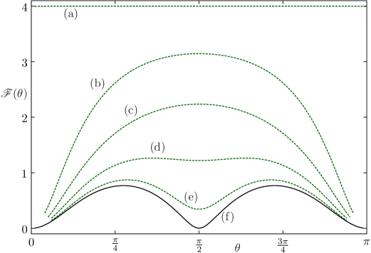
Figure 1: The Fisher information $\mathscr{F}(\theta)$ for Rob measuring the parameter $\theta$ when Alice has sent him the state using the single rail, plotted as a function of $\theta$ for various values of $r$. For line (a) $r=0.001$, which is close enough to zero to be the starting point. Lines (b), (c), (d), and (e) have $r=0.5$, $r=0.8$, $r=1.2$, and $r=1.9$ respectively. Line (f) has $r=2.8$ which we are taking to be the converged value within the approximate thickness of the line.

We can now differentiate with respect to $\theta$ and transform into the same basis,

$$\left(\rho_{AR}^{\prime(d)}(\theta)\right)_{n}=\begin{pmatrix}0&(n+1)\cot\theta\frac{\tanh^{2(n+m)}(r)}{\cosh^{6}(r)}\\ (m+1)\tan\theta\frac{\tanh^{2(n+m)}(r)}{\cosh^{6}(r)}&(m-n)\sin(2\theta)\frac{\tanh^{2(n+m)}(r)}{\cosh^{6}(r)}\end{pmatrix}.$$ (10ae)

This makes it possible to apply the lowering operator. We can then perform the multiplication and trace for each block, finally summing every block to find the Fisher information,

$$\mathscr{F}(\theta)=\sum_{n,m=0}^{\infty}2\left(2+m+n+(m-n)\cos(2\theta)\right)\frac{\tanh^{2(n+m)}(r)}{\cosh^{6}(r)}=4.$$ (10af)

This is again the maximum information possible to extract from the noiseless state. The same reasoning applies to the dual rail as to the single rail. If Alice is included in the measurement, she can always ignore Rob’s state and measure her own. The decoherence does not matter in the type of measurement she needs to do to find $\theta$. Alice is therefore capable of performing an optimal measurement regardless of any communication noise with Rob.

4 Results for amplitude estimation

We now plot the results of Rob measuring the parameter alone since these are the nontrivial results. As discussed in the previous section, if Alice assists in the measurement, she can always achieve the Fisher information of $4$. Rob, however, is affected by the noise generated in the communication channel due to his acceleration.

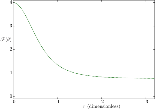
Figure 2: The Fisher information $\mathscr{F}(\theta)$ for Rob measuring the parameter $\theta$ when Alice has sent him the state using the single rail, plotted as a function of $r$ for a representative value of $\theta=\frac{\pi}{4}$.

We briefly noted in LABEL:ch:blackholes that there was an asymmetry between the $\lvert\mathnormal{0}\rangle$ and $\lvert\mathnormal{1}\rangle$ states when using the single rail. This becomes very pronounced when the parameter we are trying to measure oscillates the amplitude between the $\lvert\mathnormal{0}\rangle$ and $\lvert\mathnormal{1}\rangle$ states. The Fisher information is plotted as a function of the parameter $\theta$, for various values of $r$ in figure 1. The ends of the lines are where the numerical algorithm did not achieve the required accuracy and so have been left out of the plot. The black solid line is the limiting line as $r$ gets large.

For low accelerations (small $r$) we see a huge difference in the sensitivity of the measurement when $\theta$ is at different values. When $\theta\approx 0$ or $\theta\approx\pi$, the state is almost $\lvert\mathnormal{0}\rangle$, we see a minimum Fisher information. If $\theta\approx\frac{\pi}{2}$, the state is almost $\lvert\mathnormal{1}\rangle$ and we see a maximum. When the accelerations get larger (around $r>1$), the sensitivity decreases for both $\lvert\mathnormal{0}\rangle$ and $\lvert\mathnormal{1}\rangle$. The maximum sensitivity starts to move towards the points where they have equal amplitude.

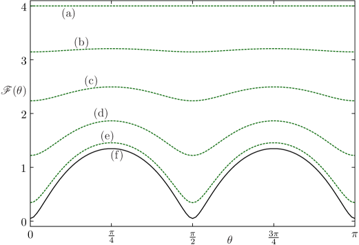
Figure 3: The Fisher information $\mathscr{F}(\theta)$ for Rob measuring the parameter $\theta$ when Alice has sent him the state using the dual rail, plotted as a function of $\theta$ for various values of $r$. For line (a) $r=0.001$, which is close enough to zero to be the starting point. Lines (b), (c), (d), and (e) have $r=0.5$, $r=0.8$, $r=1.2$, and $r=1.9$ respectively. Line (f) has $r=2.9$ which we are taking to be the converged value within the approximate thickness of the line.

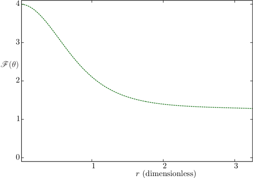
Figure 4: The Fisher information $\mathscr{F}(\theta)$ for Rob measuring the parameter $\theta$ when Alice has sent him the state using the dual rail, plotted as a function of $r$ for a representative value of $\theta=0.65$.

At low accelerations, the probability of measuring a noise excitation in the mode is very low. Therefore, if $\theta=\frac{\pi}{2}$ there is definitely at least one photon in the mode. If $\theta=0$ there are most likely to be no photons in the mode, but there is a possibility of having one photon. This gives you a higher probability of estimating the parameter correctly if $\theta=\frac{\pi}{2}$ because you will measure at least one photon and guess the correct value of $\theta$. If $\theta=0$, you have a chance of getting the estimate wrong if you do measure a noise excitation instead of the vacuum.

As the acceleration gets larger there is a transition into the region where the best sensitivity comes from the most mixed states, those where $\theta\approx\frac{\pi}{4}$ and $\theta\approx\frac{3\pi}{4}$. If the state is near a logical basis state, it becomes difficult to estimate $\theta$ due to the large amount of noise photons flooding the signal. If there are approximately equal amplitudes of each basis state, the correlations between them become important. The shift between these two behavioural regions occurs near to the acceleration for which the expected number of noise excitations is one.

We have plotted the Fisher information over $r$ for a typical value of $\theta=\frac{\pi}{2}$ in figure 2. This allows us to see how the acceleration affects the measurement sensitivity. We expect, from our calculations in LABEL:ch:blackholes and the fact that the parameter estimation is a classical information task, that the sensitivity will drop off from its noiseless maximum but tend towards a finite value for large accelerations. This is indeed reflected in the graph.

When communicating via the dual rail, there is perfect symmetry between the $\lvert\mathnormal{0}\rangle$ and $\lvert\mathnormal{1}\rangle$ states. This is clear to see in figure 3, where we have plotted the Fisher information over $\theta$ for various values of $r$. The solid black line is the limiting line as $r$ gets large.

We can see from figure 3 that again the communication noise has a variable effect depending on the parameter $\theta$. There is less sensitivity in resolving $\theta$ when the state is closer to a computational basis state. The greatest sensitivity is when the amplitudes are equal in the computational basis.

The noise in each mode is independent of the other mode. This means that correlating the two modes tends to reduce the noise. The highest sensitivity comes from when the state is correlated, and the measurement can detect these correlations. If the state is not correlated between the two modes (one of the logical basis states), it becomes an attempt to measure which mode has a higher average excitation.

To see the form of the loss of sensitivity due to acceleration, we have plotted the Fisher information over $r$ for a representative value of $\theta=0.65$ in figure 4. This value was chosen because the computational time to calculate for $\theta=\frac{\pi}{4}$ was prohibitively large. This is very similar to the form of the classical communication reduced channel capacity seen in LABEL:ch:blackholes. We see the Fisher information decrease from it’s maximal value of $4$ as $r$ increases but converge to a finite value that is larger than the convergent value of the single rail. This reflects the conclusion that the dual rail can carry more information that the single rail.

5 Using NOON states to estimate relative phase

We now study the similar situation where an inertial observer, Alice, communicates information about a parameter with a constantly accelerated observer, Rob. Alice prepares a state with $\theta=0$, which undergoes a unitary evolution that imparts the phase $\theta$ onto the state. If encoded using the dual rail, the state is,

$$\lvert\psi\rangle_{A}^{(d)}=\lvert N,\varnothing\rangle+e^{iN\theta}\lvert\varnothing,N\rangle.$$ (10ag)

This dual rail state is known as the NOON state in quantum interferometry, originally introduced by Bollinger et al. [Bollinger1996]. It encodes the parameter onto the relative phase. Equivalently, the state encoded using the single rail is,

$$\lvert\psi\rangle_{A}^{(s)}=\lvert\varnothing\rangle+e^{iN\theta}\lvert N\rangle.$$ (10ah)

This requires a fully quantum channel because if it became classical at any point, all phase information would be lost.

The task is for Rob to measure the field and obtain an estimate for the parameter $\theta$. We need to find out precisely how well he is able to perform this task. Rob’s detector will be subject to the relativistic noise present in the form of the Unruh-Hawking effect [Hawking1975, Unruh1976, Takagi1986].

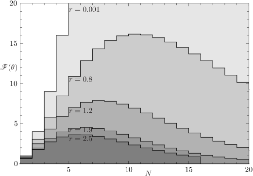
Figure 5: The quantum Fisher information $\mathscr{F}(\theta)$ plotted as a function of $N$ for Rob measuring the parameter $\theta$ when Alice has sent him the state using the single rail for various values of $r$.

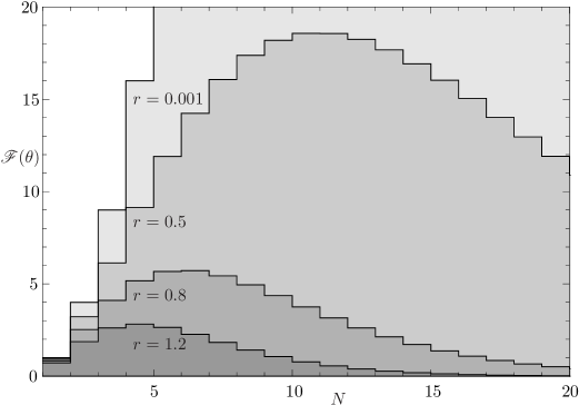
Figure 6: The quantum Fisher information $\mathscr{F}(\theta)$ plotted as a function of $N$ for Rob measuring the parameter $\theta$ when Alice has sent him the state using the dual rail for various values of $r$.

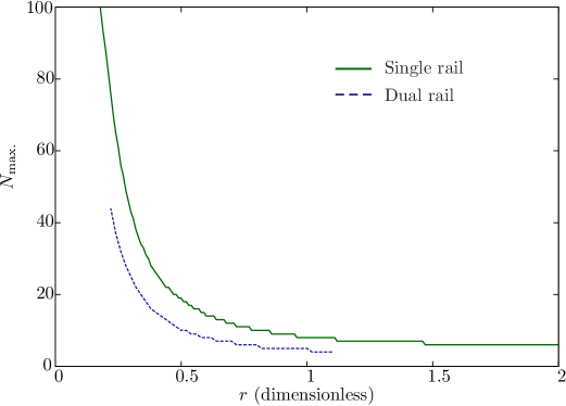
Figure 7: The value of $N$ resulting in a maximum quantum Fisher information $\mathscr{F}(\theta)$ for Rob measuring the parameter $\theta$ when Alice has sent him the state using the single rail plotted as a function of $r$ for both the single rail and dual rail. The dual rail has a shorter line because the computational resources required prohibited further calculation in either direction.

Once Alice has created the state, she no longer has access to it. Rob must then measure the field to determine the parameter. To find out what Rob can measure, we must describe the field in terms of his mode functions LABEL:sec:fields:transformation. As in LABEL:ch:blackholes, we use the Single Wedge Mapping, where Alice creates Unruh modes that directly map to Rindler modes in Rob’s Rindler wedge, see Chapter 11. When we apply the squeezing transformation given in LABEL:eq:fields:twomodesqueezing to a mode with N excitations present $\lvert\psi\rangle_{A}=\lvert N\rangle$, the transformed state in both Rob and anti-Rob’s bases is,

$$\lvert\psi\rangle_{R\bar{R}}=\sum_{p=0}^{\infty}\frac{(ir)^{p}}{|r|^{p}}\frac{\tanh^{p}|r|}{\cosh^{N+1}|r|}\begin{pmatrix}p+N\\ p\end{pmatrix}^{\frac{1}{2}}\lvert N+p\rangle_{R}\otimes\lvert p\rangle_{\bar{R}}.$$ (10ai)

To transform the full states, we construct Alice’s density matrix from the states with zero and $N$ excitations, then transform each term according to equation 10ai. Finally, we trace out anti-Rob leaving Rob with a mixed state represented by an infinite matrix in the number basis.

To calculate the quantum Fisher information numerically we need a finite matrix. The coefficients of the matrix decay as the number of excitations increases. We can therefore use a truncation of the matrix to get the result within a specified precision. We numerically evaluated the matrices, for a size $k$, and calculated the quantum Fisher information. To check that the truncated size was sufficient, we calculated the quantum Fisher information for matrices of size $k+1$. We continued to increase $k$ until the quantum Fisher information changed less than the prescribed precision.

Using this truncated matrix, $\rho$, we calculated the quantum Fisher information using the algorithm as follows.

1. Find eigenvalues and eigenvectors of $\rho$.

2. Differentiate $\rho$ with respect to $\theta$ to find $\rho^{\prime}$.

3. Use the eigenvectors of $\rho$ to transform both $\rho$ and $\rho^{\prime}$ into the basis where $\rho$ is diagonal.

4. Perform the lowering operator according to LABEL:eq:inf:loweringoperator.

5. Calculate the quantum Fisher information using the trace of the matrix product of $\rho^{\prime}$ and the lowered $\rho^{\prime}$.

The quantum Fisher information includes $\theta$ in its calculation, however the final result does not depend on $\theta$. We set $\theta=0.65$ throughout this section. The quantum Fisher information does depend on both $r$, the squeezing parameter, and $N$, the number of excitations Alice created in the states.

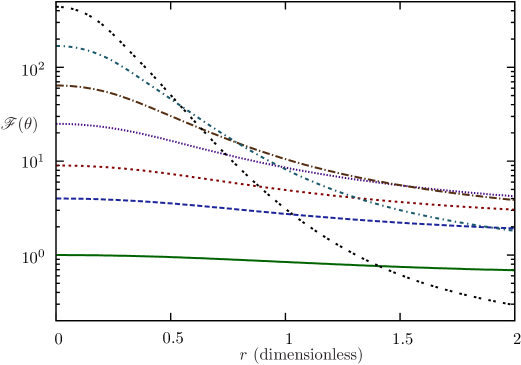
Figure 8: The quantum Fisher information $\mathscr{F}(\theta)$ plotted as a function of $r$ for Rob measuring the parameter $\theta$ when Alice has sent him the state using the single rail. The values of $N$ for each line are $1$, $2$, $3$, $5$, $8$, $13$ and $21$, corresponding to increasing Fisher information for $r=0$.

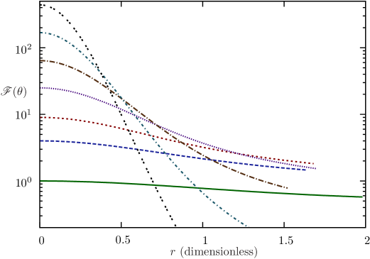
Figure 9: The quantum Fisher information $\mathscr{F}(\theta)$ plotted as a function of $r$ for Rob measuring the parameter $\theta$ when Alice has sent him the state using the dual rail. The values of $N$ for each line are $1$, $2$, $3$, $5$, $8$, $13$ and $21$, corresponding to increasing Fisher information for $r=0$.

6 Results for phase estimation

The quantum Fisher information is shown against $N$ for various values of the parameters, in figure 5 for single rail encoding, and in figure 6 for dual rail encoding. The channel is similar to an amplifying channel in that the more excitations that are present initially the more excitations are created by the channel. Because the excitations created by the channel are thermal, they contribute to a higher noise level. If there is a higher number of initial excitations there is more noise. We find an exponential decay in the quantum Fisher information with respect to, $N$, the initial number of excitations, for a fixed acceleration. This results in an optimal value of $N$ to use for each particular noise level. Higher $N$ states sent via the dual rail are more susceptible to the noise than the single rail equivalents. This is due to the fact that both the logical zero and logical one contain $N$ excitations, whereas in the single rail, the zero contains no excitations. This results in a smaller expected number of excitations for the single rail, and hence less noise.

In LABEL:ch:blackholes and 9, we found the dual rail channel to perform better than the single rail for quantum communication between inertial Alice and accelerated Rob. Here we find the opposite effect, that the single rail channel performs better. These studies may use similar states, however, they are measuring a different quantity. The information in the states studied previously was contained in the relative amplitude of the logical zero and one basis states. In this study, the information about $\theta$ is contained entirely in the relative phase. Whilst perhaps surprising, it is not impossible that different encoding methods are favoured for these situations.

The optimal value of $N$ is shown against $r$ in figure 7 for the single rail. We expect it to be asymptotic as $r\to 0$ because at $r=0$, $\mathscr{F}(\theta)=N^{2}$. The fact that it drops at all is perhaps surprising because it is known for noiseless situations that NOON states are optimal [Bollinger1996]. Using NOON states in a noiseless situation results in a Fisher information that scales with $N^{2}$.

For zero noise, the quantum Fisher information rises with $N^{2}$. When there is noise present, there is an exponential decay reducing the quantum Fisher information for larger $N$. To match this physical situation, we fitted this for each value of $r$ with a model of the form,

$$\mathscr{F}(\theta)=N^{2}e^{-a(r)N+b(r)}.$$ (10aj)

We found that for each $r$, this functional form fitted very well. For large $r$, the coefficient $a(r)$ tended towards a linear function of $r$. This function has a gradient of $(41.6\pm 0.3)\times 10^{-3}$, when calculated using data for which $2.08\leq r\leq 3.10$. It would be possible to use the linear dependence of the fitting parameter $a(r)$ to find the maximum value of $N$ for large $r$. However, the interesting behaviour happens near $r=1$, because this is where the expected number of noise excitations is approximately $1$.

The quantum Fisher information is shown as the noise increases for various values of $N$ in figures 8 and 9 for the single and dual rails respectively. Due to the large computational requirements of calculating these graphs, some of the lines stop before the end of the graph. The quantum Fisher information decreases with increasing noise for each value of N, which is expected behaviour. It is clear from the graphs that the single rail performs better than the dual rail for all values of $r$.

7 Conclusion

In this chapter we studied the parameter estimation capabilities of Alice and Rob once the state encoding the parameter had passed through a quantum communication channel. We looked at different types of states, ones similar to states used in LABEL:ch:blackholes, and NOON states.

1 Amplitude estimation

The protocol used in the first part was where Alice encoded the parameter onto her state, then created entanglement with Rob followed by a measurement performed by one or both of them to determine the parameter $\theta$. If Alice is involved in the measurement, she can always perform an optimal measurement as expected. This is true regardless of what communication happened with Rob, the optimal measurement is the one where Alice discards any measurement from Rob and just uses her own subsystem. This allows her the full Fisher information of $\mathscr{F}(\theta)=4$ every time.

For Rob to measure alone, after performing this channel, we first discard Alice’s subsystem, giving Rob a mixed state. When Rob measures this mixed state, the Fisher information degrades with increased channel noise. Rob’s sensitivity to measuring $\theta$ also becomes dependent on the value of $\theta$ itself. Certain state configurations are better at protecting the information they contain from the noise present in the communication channel. This is due to the fact that we have used $\theta$ as the amplitude on a number basis encoding. The dual rail has a much higher Fisher information than the single rail, which we also expect, given the reduced classical communication capacity. However, the extractable information is highly dependant on both the value of $\theta$ and the choice of single or dual rail encoding. This suggests that the techniques used are very sensitive to particular conditions. Any application would need to have prior information of what the value of $\theta$ may be to choose the correct encoding.

The degradation of information with acceleration follows the same pattern as with classical communication in LABEL:ch:blackholes. We expect this similarity because the communication protocols used are almost identical. In both cases, we take a state encoded onto a logical basis given by the single or dual rail encodings, where the information is present in the amplitudes of the basis states. We then create entanglement between Alice and Rob using this state, followed by Rob performing any operations or measurements on his subsystem. The Fisher information measures the accuracy to which a continuous variable can be determined. The reduced classical channel capacity that we were studying in LABEL:ch:blackholes is a measure of the amount of discrete information extractable from the message. The entanglement-generating communication channel between an inertial observer and an observer hovering near a black hole degrades both continuous variable information in a similar way than it degrades discrete information.

2 Phase estimation using NOON states

The previous study was limited to single excitation states, and to a communication protocol that created entanglement between Alice and Rob. In the second part of this chapter we extend the work to NOON states, using a communication protocol where Alice simply sends the state to Rob. There is no entanglement generated so Alice does not need to be traced out, which preserves phase information in Rob’s subsystem.

The channel used is amplifying in nature; the noise is dependent on the number of excitations already present. Because of this $N$-dependent noise, there exists an optimum $N$ for maximum information transfer. The $N$ dependence of the quantum Fisher information has a simple form which we fitted numerically. The coefficients of the fit are dependent on $r$, the squeezing parameter, as expected. We found that the decay coefficient had asymptotically linear dependence on $r$. This could allow extrapolation to any noise levels. The decay of the quantum Fisher information with noise was monotonic regardless of any possible optimisation over NOON states, as expected.

We find in this case that the single rail outperforms the dual rail. Whilst further research would be required to ascertain exactly why, the main differences are as follows. In this study, we used the parameter encoded onto the phase rather than the amplitude. The single and dual rail encodings may be better suited to preserving these different types of information. The communication protocol was different, Alice simply sent the state to Rob rather than generating an entangled version of the state.

3 Implications

The study of metrology is important to direct technological techniques for measuring physical parameters. Any measurement protocols using these types of fields under accelerated conditions would need to use this knowledge to tailor their encodings specifically to the parameters they are measuring. We have studied the effect on extractable information about a continuous variable under accelerated conditions. Continuous variable quantum computing may benefit from knowing what encodings of the variables maintain the best information in these situations.

Further work would include studying other forms of states to find more optimal information transfer. There has been work on lossy interferometry using states of other forms, where these states are more robust to the noise than NOON states [Maccone2008, Knysh2011]. We expect a higher quantum Fisher information to be possible in this situation in a similar way. The noise here has a similar $N$ dependence to the errors in lossy channels.

Chapter 9 Communication between inertial and causally disconnected, accelerated agents

We study a different situation in this chapter. LABEL:ch:blackholes and LABEL:ch:measure looked at Alice, an inertial observer, sending information to Rob only, who was undergoing constant acceleration or hovering above a black hole. We approximated the field in Rob’s frame using the Rindler modes. In this chapter, we take the Rindler setup, and study the communication between two pairs of observers: An inertial observer, Alice ($A$) and two constantly accelerated complementary observers Rob ($R$) and AntiRob ($\overline{R}$). The complementary observers move with opposite accelerations in the two causally disconnected regions of the Rindler spacetime, the same setting as in [Bruschi2010]. This setting is depicted in figure 1. This chapter is based on a paper prepared in collaboration with Eduardo Martín-Martínez and Miguel Montero [Martin-Martinez2012a].

Figure 1: This figure depicts Alice as an inertial observer in the centre. Rob and AntiRob are depicted accelerating away from each other.

1 Introduction

In LABEL:ch:blackholes and LABEL:ch:measure we used the the Single Wedge Mapping (SWM, discussed in Chapter 11) as we believed it to be optimal for the communication we studied between Alice and Rob. Here, we discover that for classical communication at high accelerations this is not the case: we must go beyond the SWM to reach optimal communication. The channels we study are the bipartite Alice-Rob and Alice-AntiRob channels. It is not necessary to study any Rob-AntiRob channel because they are causally disconnected; no communication is possible. We must also go beyond the SWM to deal with communication between Alice and AntiRob.

We discuss that for families of states built from Unruh modes, Alice and different non-inertial observers may not be able to generate entanglement using the state merging protocols (see LABEL:subsec:inf:statemerging) with these quantum channels. In other words, when preparing the field state, Alice will have to choose with whom she wants to generate entanglement, since some of the states that she can prepare will not allow entanglement generation with some of the non-inertial observers. We will show the monogamy property for the Unruh mode-based entanglement generation mentioned above when we go beyond the SWM.

2 Setting

We will analyse here the information flow for both the single rail and dual rail encoding methods. The single rail uses a single field mode, representing a logical zero with the vacuum and a logical one with a single excitation. The dual rail uses two field modes with an excitation in one or the other to represent logical zero and logical one. These encoding methods have been discussed in LABEL:sec:inf:encoding.

We study here restricted channel capacities (see LABEL:subsec:inf:quantumchannelcapacity) because we confine ourselves to either the single rail or dual rail encoding methods. To study these restricted capacities, we must optimize over all parameters and encodings controlled by either Alice or Rob, obtaining optimal achievable rates by these encodings methods. Alice has the freedom to choose which field mode to excite to send the best message to Rob. We will not consider the possibility of Alice or Rob using arbitrary elements of the Fock space, as this would mean an infinite number of optimization parameters; we will stick to the simpler case of single field modes excited just once. Rob is still allowed to measure within the full Fock basis of his mode, as this allows him to extract the information required.

3 Field state

Alice creates the appropriate excitations, once she knows which observer she would like to communicate with, and what their acceleration is. As discussed in LABEL:subsec:inf:quantuminfomeasures, the classical message is a probabilistic mixture of logical zero and logical one states, and the quantum message is a particular qubit where the state merging protocol is then used to generate entanglement. These excitations will be given by, equation 10aa for classical communication and equation 10ab for quantum communication, respectively,

$$\sigma_{A}(\mbox{general bit})= \left\lvert\alpha\right\rvert_{\text{}}^{2}\left\lvert\mathnormal{0}\right\rangle_{A}\prescript{}{}{\left\langle\mathnormal{0}\right\rvert}+\left\lvert\beta\right\rvert_{\text{}}^{2}\left\lvert\mathnormal{1}\right\rangle_{A}\prescript{}{}{\left\langle\mathnormal{1}\right\rvert},$$ (10aa)

$$\rho_{A}(\mbox{general qubit})= \left(\alpha\left\lvert\mathnormal{0}\right\rangle_{A}+\beta\left\lvert\mathnormal{1}\right\rangle_{A}\right)\otimes\left(\alpha\prescript{}{A}{\left\langle\mathnormal{0}\right\rvert}+\beta\prescript{}{A}{\left\langle\mathnormal{1}\right\rvert}\right).$$ (10ab)

Again, we use the parameter values $\left\lvert\alpha\right\rvert_{\text{}}^{2}=\left\lvert\beta\right\rvert_{\text{}}^{2}=\frac{1}{2}$ for the majority of this chapter. This is optimal for dual rail which is verified numerically here, and provides representative behaviour for single rail communication. We discuss the effect on the optimisation if we allow $\alpha$ and $\beta$ to be free variables again in Section 5. We then perform the transformation into the accelerated frame as specified in LABEL:sec:fields:transformation. AntiRob’s frame is not traced out because we need to calculate information quantities in the Alice-AntiRob bipartition.

I present here the full state of the field for the four communication methods. For classical communication, the field is given by,

$$\sigma_{AR\overline{R}}=\left\lvert\alpha\right\rvert_{\text{}}^{2}\left|\Psi\middle\rangle\middle\langle\Psi\right|+\left\lvert\beta\right\rvert_{\text{}}^{2}\left|\Phi\middle\rangle\middle\langle\Phi\right|$$

and for quantum communication, by,

$$\rho_{AR\overline{R}}=\left(\alpha\left\lvert\Psi\right\rangle+\beta\left\lvert\Phi\right\rangle\right)\otimes\left(\alpha^{*}\prescript{}{}{\left\langle\Psi\right\rvert}+\beta^{*}\prescript{}{}{\left\langle\Phi\right\rvert}\right)$$ (10ba)

where, the $$\lvert\Psi\rangle \lvert\Phi\rangle \left\lvert A,R,\overline{R}\right\rangle$$ and depend on the encoding methods. In the single rail, using the basis these are given by,

$$\lvert\Psi\rangle^{(s)}= \sum_{n}\frac{\tanh^{n}r}{\cosh r}\left\lvert 0,n,n\right\rangle,$$ (10bb)

$$\lvert\Phi\rangle^{(s)}= \sum_{n}\frac{\tanh^{n}r}{\cosh^{2}r}\sqrt{n+1}\sum_{p=0}^{1}q_{\text{L}}^{1-p}q_{\text{R}}^{p}\left\lvert 1,n+p,n+1-p\right\rangle.$$ (10bc)

In the dual rail, using the basis $$\left\lvert A,R_{\mathnormal{0}},R_{\mathnormal{1}},\overline{R}_{\mathnormal{0}},\overline{R}_{\mathnormal{1}}\right\rangle$$ these are given by,

$$\lvert\Psi\rangle^{(d)}= \sum_{n,m}\frac{\tanh^{n+m}r}{\cosh^{2}r}\sqrt{n+1}\sqrt{m+1}\sum_{p=0}^{1}q_{\text{L}}^{1-p}q_{\text{R}}^{p}\left\lvert 0,n+p,m,n+1-p,m\right\rangle,$$ (10bd)

$$\lvert\Phi\rangle^{(d)}= \sum_{n,m}\frac{\tanh^{n+m}r}{\cosh^{2}r}\sqrt{n+1}\sqrt{m+1}\sum_{p=0}^{1}q_{\text{L}}^{1-p}q_{\text{R}}^{p}\left\lvert 1,n,m+p,n,m+1-p\right\rangle.$$ (10be)

The dual rail has a clear symmetry between the zero and one modes because the form of $\lvert\Psi\rangle$ and $\lvert\Phi\rangle$ are the same. There is symmetry under the exchange of $q_{\text{R}}$ with $q_{\text{L}}$ and Rob with AntiRob, so without loss of generality we need only study Rob as a receiver. This allows us to trace out AntiRob simplifying the density matrix.

Beyond the Single Wedge Mapping, ($q_{\text{R}}<1$) the relevant density matrices are no longer block diagonal and they cannot be diagonalized into a closed form, as was shown by Bruschi et al. in [Bruschi2010]. This forced us to calculate the matrix representations in the Fock basis of the full field state in Matlab [Matlab] with truncation at a matrix size of $k\times k$. The partial traces and diagonalisation required were performed numerically, and the sums calculated for the entropic quantities. This was done for many different values of $k$ until it was established that we had $k$ large enough such that the error introduced was sufficiently small.

4 Classical communication

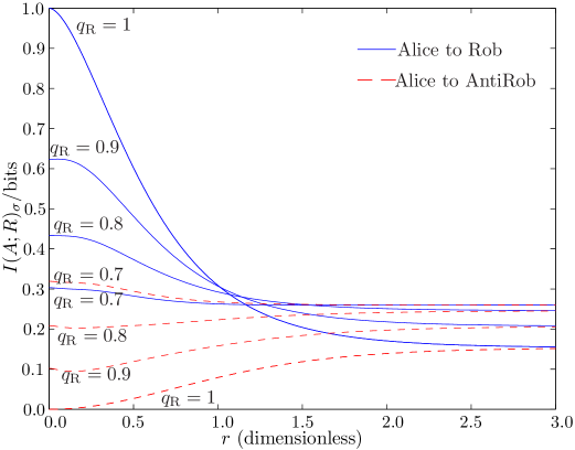
Figure 2: Holevo information plotted as a function of $r$ of the single rail method of classical communication for various values of $q_{\text{R}}$.

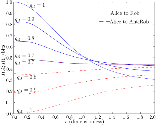
Figure 3: Holevo information plotted as a function of $r$ of the dual rail method of classical communication for various values of $q_{\text{R}}$.

The restricted classical channel capacity is given by the Holevo information maximized over controllable parameters. This has been calculated and plotted for both the single rail encoding in figure 2 and the dual rail encoding in figure 3. We see from the plots that for large acceleration the maximum Holevo information is not achieved for $q_{\text{R}}=1$ (Single Wedge Mapping). This shows that the assumptions made in the previous chapter are not correct for larger accelerations. While it is true that SWM maximizes classical communication for low accelerations, for large accelerations we need to go beyond the SWM to achieve the restricted capacity.

Classical communication tends to a finite value for large accelerations (equivalent to large $r$), which is larger for dual rail communication. No matter what the value of $q_{\text{R}}$ we find that as acceleration increases it is possible for Alice to communicate with both Rob and AntiRob. At large accelerations Alice has equal communication channel capacity with both Rob and AntiRob, which is optimized at $q_{\text{R}}=\frac{1}{\sqrt{2}}$.

Note from figures 2 and 3 that, at infinite acceleration, the Holevo information of the Alice-Rob and Alice-AntiRob channels both converge to the same value. This is easily understood by looking at LABEL:eq:fields:unruh-general-annihilation and the definition of $\hat{a}_{\text{U}_{\text{L}}}$ and $\hat{a}_{\text{U}_{\text{R}}}$ in LABEL:eq:fields:UrandUl, and noting that at infinite acceleration both $\sinh r$ and $\cosh r$ tend to $e^{r}/2$, and therefore in this limit LABEL:eq:fields:unruh-general-annihilation may be written as,

$$\hat{a}_{\text{U}}\approx\frac{e^{r}}{2}\left[q_{\text{R}}\hat{a}_{\text{R}_{\text{I}}}-q_{\text{R}}\hat{a}_{\text{R}_{\text{IV}}}^{\dagger}+q_{\text{L}}\hat{a}_{\text{R}_{\text{IV}}}-q_{\text{L}}\hat{a}_{\text{R}_{\text{I}}}^{\dagger}\right].$$ (10bc)

This expression is invariant under the replacements $\text{I}\leftrightarrow\text{IV}$ and $q_{\text{L}}\leftrightarrow q_{\text{R}}$, which takes Rob to AntiRob and vice-versa, and therefore in the infinite acceleration limit the Holevo information of both bipartitions must be the same. In this limit, there is maximal squeezing between Rob and AntiRob’s modes. For Alice’s message to be received well by either or both Rob and AntiRob then she must have it evenly spread between the two. This ensures that both regions of spacetime have the message present, so when they mix, there is still the message. If Alice only put the message in one region, then with maximal squeezing it would get mixed with the region where there was no message and get lost. This also explains, why at large accelerations the parameter values $q_{\text{R}}=q_{\text{L}}=\frac{1}{\sqrt{2}}$ are optimal.

5 Optimising over $q_{\text{R}}$ and $\alpha$

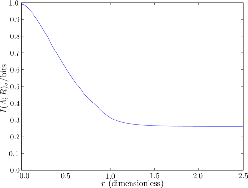
Figure 4: Optimal Holevo information as a function of the acceleration in the single rail case.

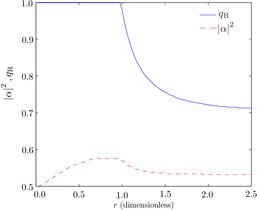
Figure 5: $\left\lvert\alpha\right\rvert_{\text{}}^{2}$ and $q_{\text{R}}$ optimal parameters for the results plotted in figure 4.

The optimal value of $q_{\text{R}}$ is $1$ for low acceleration, and $q_{\text{R}}=\frac{1}{\sqrt{2}}$ for high acceleration. It is interesting to study the behaviour of the optimal parameter values between these two regimes. We take the single rail encoding as the example because the computation time of numerically optimising over different $q_{\text{R}}$ in the dual rail encoding is prohibitive. As mentioned in LABEL:ch:blackholes, there is an asymmetry in the single rail encoding. We also noted the large variation of the quantum Fisher information as the parameter changed the state between the logical basis states in the single rail encoding in Section 1. It is interesting to study the behaviour of the optimum value for $\alpha$ in the single rail encoding. We perform a two dimensional optimisation here over these two parameters.

We have plotted the optimal Holevo information which is the restricted channel capacity for the classical single rail case in figure 4. Figure 5 shows the optimal values of $(\left\lvert\alpha\right\rvert_{\text{}}^{2},q_{\text{R}})$ used for each point on figure 4. We see that the Single Wedge Mapping is optimal up to $r\approx 1$. Note the interesting non-monotonic behaviour of the parameter $\left\lvert\alpha\right\rvert_{\text{}}^{2}$ which starts at approximately the same time $q_{\text{R}}=1$ becomes non-optimal. This parameter is always close to $\frac{1}{2}$, but slightly biased to higher values. This is due to the asymmetry in the noise when using the single rail method.

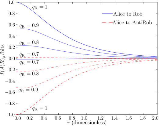
Figure 6: Coherent information of the single rail method of quantum entanglement generation.

6 Quantum communication and entanglement generation

The quantum coherent information is given by the negative of the conditional entropy. The results of this were plotted for both the single rail in figure 6 and the dual rail in figure 7.

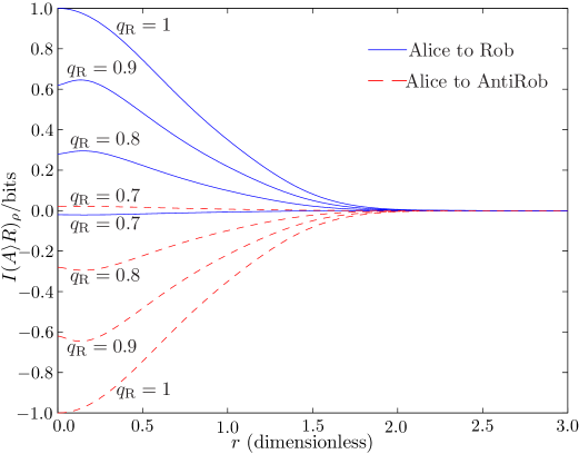
Figure 7: Coherent information of the dual rail method of quantum entanglement generation.

The plots show that when the coherent information is positive for one bipartition, it is negative for the other. We call this the monogamy property, Alice must choose in advance with whom she wants to generate entanglement for quantum communication. For large acceleration, the coherent information tends to zero, for both single rail and dual rail methods. The dual rail methods always perform slightly better than the single rail methods.

We find that beyond the Single Wedge Mapping the decrease in information transfer is non-monotonic. However, in most cases this is not optimal, as Alice is able to choose her modes, and therefore has control over the value of $q_{\text{R}}$. This means that, after the maximization, the restricted capacities are monotonically decreasing with the acceleration parameter. The SWM is sufficient to fully describe optimal entanglement generation for all accelerations. In LABEL:ch:blackholes, the interesting entanglement generation results used the SWM, which we have verified here is appropriate.

We find that if one of the channels is able to generate entanglement, the other cannot. More precisely, the sum of the conditional entropies of both channels is always greater than or equal to zero. This is a consequence of the strong subadditivity of the von Neumann entropy [Lieb1973], which implies that for any tripartite system composed of parties $A$, $B$ and $C$, the inequality,

$$S(\rho_{A})+S(\rho_{C})\leq S(\rho_{AB})+S(\rho_{BC}),$$ (10bd)

holds. Choosing $A=\text{AntiRob}$, $B=\text{Alice}$, $C=\text{Rob}$ and rearranging, we obtain this condition on the sum of conditional entropies,

$$[S(\rho_{A\bar{R}})-S(\rho_{\bar{R}})]+[S(\rho_{AR})-S(\rho_{R})]\geq 0.$$ (10be)

If Alice can generate quantum entanglement with Rob, she will not be able to do the same with AntiRob, and vice versa. The results we are presenting saturate the inequality equation 10be, but the interpretation is the same: the entanglement generation ability of the state merging protocol is bound to be zero for at least one of the bipartitions.

7 Conclusion

We have studied the classical Holevo information and the quantum conditional information (both in the single and dual rail encodings) in the situation where an inertial observer (Alice) communicates by sending information to two counter-accelerating observers each outside of the other’s acceleration horizon (Rob and AntiRob). The dual rail encoding has consistently outperformed the single rail for both classical and quantum channel capacities in this setting. The dual rail is symmetrical between the logical basis states. The noise generated in each mode is independent but equal in magnitude and therefore the resulting state is symmetrical. The single rail uses only one mode, and therefore there are differences between the logical basis states. They acquire potentially different levels of noise. We saw that the optimal values of the parameters deviate from symmetry.

We found that the quantum channels between the inertial observer and each of the accelerated observers are mutually exclusive. Alice must choose with which accelerated observer, Rob or AntiRob, she wants to generate entanglement. This is not simply a demonstration of the no-cloning theorem because the monotony holds for separate messages on separate occasions, if Alice uses the same setup. The setup used to communicate with Rob cannot ever be used to communicate with AntiRob, the values of $q_{\text{R}}$ and $q_{\text{L}}$ need to change. If we wanted to design technology to communicate quantum information between inertial and accelerated observers, we would have to design some way of changing the mode functions to which it couples. A fixed mode function coupling would only ever allow quantum communication with observers that have certain specific characteristics. We may need some sort of ‘tuning’ mechanism that allows Alice to switch her communication channel from Rob to AntiRob. Classical communication is not affected by this limitation. We find again, that classical information and correlations are more robust, and allow Alice to communicate with both Rob and AntiRob using the same channel.

We showed that an Unruh mode with $q_{\text{R}}=1$ is always optimal to send quantum information to Rob and $q_{\text{R}}=0$ is optimal for communication with AntiRob. For larger acceleration, and therefore larger $r$, we find that $q_{\text{R}}=1$ is no longer optimal for sending classical information to Rob, in both the single and dual rail encodings. This is important for other research in the field because the single wedge approximation (of $q_{\text{R}}=1$) is very commonly used. Researchers must understand the limitations of using this approximation, and in what situations it no longer provides an optimal channel. The main conclusions do not change however, from extending beyond the approximation. The channel still remains finite in the infinite acceleration limit. We have computed the optimal $\left\lvert\alpha\right\rvert_{\text{}}^{2}$ and $q_{\text{R}}$ for the single rail encoding, showing that the corresponding Holevo information is a monotonically decreasing function of the acceleration. This monotonical decrease is important because it would be very surprising to have the channel increase again for increased noise levels.

The encodings of single and dual rail have restricted the states used in the channel. The communication may be improved if we were to use a different computational basis, perhaps not using the number basis at all. We could use some states that are common in metrology, such as the NOON state, or other multi-excitation states.

We could also study the situation using a broadcast channel formalism. Instead of treating it as separate communication attempts, using the same system setup, we could investigate simultaneous communication between Alice, Rob and AntiRob. Causality would prohibit Rob and AntiRob from communicating at all, but Alice could simultaneously send classical and quantum information to both of them.

Chapter 10 Conclusion

Both quantum communication and metrology will be very relevant to technology in the coming years. Quantum computing is getting closer, and with it the need for quantum communication. Metrology has always been relevant to perform the most precise measurements possible. Using quantum effects in metrology can increase the precision beyond what is possible classically. When these technologies are used in situations where they are subject to acceleration or a gravitational field it is important to understand how their behaviour will change. Studying what encodings and techniques perform the task most successfully will drive the design of this technology, particularly when it is intended to be used under similar conditions.

In this thesis we have studied relativistic quantum communication. We started by introducing the important areas of relativistic field theory and quantum information, then reviewed the field of relativistic quantum information. The focus of the thesis is communication between an inertial and an accelerated observer. We have looked at both single and dual rail encodings using bosonic field modes in all situations. The main points that have been studied are classical and quantum communication using a quantum channel between inertial Alice and Rob both accelerated and hovering above a black hole, the situation where Alice communicates with both accelerated Rob and his causally disconnected (counter-accelerated) partner AntiRob, and the ability of Rob to recover information about a continuous parameter has also been studied in the accelerated case. Time dilation is ignored in the entire thesis because it only affects the rate of communication, and of all channels equally.

Throughout the communication studies we found that the classical information was always much more robust to the noise generated by the acceleration. This is demonstrated by the fact that the classical channel capacity remains finite all the way up to the horizon, where the quantum channel capacity drops to zero. The quantum communication is further restricted in the case where Alice uses the same setup to communicate with both Rob and AntiRob. This restriction is that Alice can tune her communication device to either have a non-zero quantum capacity with Rob or AntiRob, but not both. For parameter estimation, we find a similar situation to classical communication, in that the amount of extractable information tends towards a finite value as the acceleration increases. Using the entanglement generating communication protocol with the parameter encoded onto the amplitudes, this limiting value is highly dependent on the particular encoding (single or dual rail) and the value of the parameter itself.

For the majority of the thesis, we use the single wedge mapping because it often provides the optimal information transfer. Quantum communication remains optimal in the single wedge mapping in all situations that we studied. However, we found for classical communication with an accelerated observer that it is no longer optimal. The main conclusions do not change, only the limiting value of the classical channel capacity. This should not affect the metrology chapter because the information transfer is fully quantum, where we continued to find the single wedge mapping optimal. It is important to understand the limitations of such simplifications, particularly when they are heavily used in the literature.

The dual rail encoding provided greater information transfer in almost all situations studied. Estimating the phase of a NOON state after communication through the quantum channel had better precision when using the single rail. This was unexpected but perhaps not too surprising. Their are some fundamental differences to the two techniques that are worth noting. In the situations where the dual rail was preferable, the communication was based on creating entanglement between Alice and Rob. It also stored the information in the amplitudes of the logical basis. The single rail was preferable when the communication did not create any entanglement, when it simply transferred the state to Rob. In this case we also put the parameter containing the information in the phase of the state. Further investigation would be required to determine the exact cause of this discrepancy. It is important for further research and the design of quantum communication technology to know which of these performs better in any given situation. If we could ascertain the fundamental cause of this preference, we would be able to find the optimal encoding for other situations. We may even get ideas for other encodings that could outperform both the single rail and dual rail.

In all situations we find that the information task has a monotonically decreasing ability with noise. There is no case where we suddenly have more noise in the system, and more information. This is exactly as expected.

We find that the channel we use behaves like an amplifying channel. The number of noise excitations that are created depend on the number of excitations already present in the mode. This was only noticeable when we studied NOON states with different numbers of excitations. For large $N$, the extractable information dropped to zero, because the channel became flooded with noise. This combined with the noiseless situation of a higher $N$ providing better precision meant that there was an optimal $N$ for each noise level. This may reflect back to the communication channel capacities, if we define the logical basis to be the two parts of a NOON state. We found this situation very similar to that of using NOON states in lossy interferometers that have been studied by other people. They found that replacing the NOON states with other forms of states was optimal. It would be interesting to see if those other states also improved on NOON states in this situation.

The field of relativistic quantum information theory is still quite new. Entanglement seems to have been the favourite topic so far, studied under many conditions. This work extends the field into quantum communication and metrology by studying the effect of an accelerated observer on the standard protocols. It provides many pointers for areas that may prove interesting to study. It would always be interesting to reflect the situations in which entanglement has been studied, and look at the full communication protocols. The metrology is also important because it tells us how well we can measure quantities in the situation studied. This all contributes to a greater understanding of how quantum information behaves under the influence of curved spacetimes.

Chapter 11 The Single Wedge Mapping

I call this choice of parameters the Single Wedge Mapping (SWM). This is because it reflects the fact that Alice creates Unruh mode excitations that map directly to only one of the Rindler wedges. Previously in the literature, this has been called the Single Mode Approximation. Even when we go beyond the single wedge mapping, we are still using single Rindler modes (of a single frequency) so this nomenclature is misleading. I propose to change the name and call it the single wedge mapping instead.

To set up the transformation between an inertial packet and the accelerated observers, we must first start with an annihilation operator of a Minkowski packet $\hat{a}_{\text{U}}$. We then transform it to the annihilation operators of Unruh modes, $\hat{a}_{\text{U}_{\text{L}}}$ and $\hat{a}_{\text{U}_{\text{R}}}$ for the left and right regions respectively, using the most general transformation,

$$\hat{a}_{\text{U}}=q_{\text{L}}\hat{a}_{\text{U}_{\text{L}}}+q_{\text{R}}\hat{a}_{\text{U}_{\text{R}}},$$ (10ba)

where $\left\lvert q_{\text{L}}\right\rvert_{\text{}}^{2}+\left\lvert q_{\text{R}}\right\rvert_{\text{}}^{2}=1$ and the appropriate expressions for the operators $\hat{a}_{\text{U}_{\text{L}}}$ and $\hat{a}_{\text{U}_{\text{R}}}$ for the scalar case are,

$$\hat{a}_{\text{U}_{\text{R}}} =\cosh r\,\hat{a}_{\text{R}_{\text{I}}}-\sinh r\,\hat{a}^{\dagger}_{\text{R}_{\text{II}}},$$ (10bba)

$$\hat{a}_{\text{U}_{\text{L}}} =\cosh r\,\hat{a}_{\text{R}_{\text{II}}}-\sinh r\,\hat{a}^{\dagger}_{\text{R}_{\text{I}}},$$ (10bbb)

where $\hat{a}_{\text{R}_{\text{I}}}$, $\hat{a}_{\text{R}_{\text{II}}}$ are Rindler particle operators for the scalar field in each region.

The values of $q_{\text{R}}$ and $q_{\text{L}}$ are set by the specific shape of the packet function. The inertial observer therefore has control over it, and in certain protocols we assume that $q_{\text{R}}=1$. This assumption is what I am calling the Single Wedge Mapping (SWM). When things are discussed where $q_{\text{R}}\neq 1$, this has been called ‘beyond the Single Mode Approximation’ [Bruschi2010]. I will adapt the nomenclature for this situation to ‘beyond the Single Wedge Mapping’.

In our work on black holes, LABEL:ch:blackholes and LABEL:ch:measure, we use the SWM because it broke the symmetry between Rob and AntiRob. We thought that only mapping Alice’s packet to Rob’s wedge mode would optimise the information transfer between Alice and Rob. Surprisingly, this turned out not to be the case for classical communication in the regime of large accelerations. The optimal classical communication is actually slightly higher in this regime if you move beyond the SWM.

We moved beyond the SWM in our work researching the channels between Alice, and either Rob or AntiRob, Chapter 9. To study any communication between Alice and AntiRob, we must move beyond the SWM to set up correlations between Alice and AntiRob. It was in this paper where we discovered that the SWM was not sufficient for classical communication at large accelerations.

Chapter 12 Rindler modes

Solving the Klein-Gordon equation in Rindler coordinates gives separate solutions for each region of the Rindler spacetime. The modes given here are single frequency modes as observed by the Rindler observer travelling on the path $\xi=\frac{1}{a}$.

The modes from region I are written using the Rindler equivalent of the tortoise coordinate $\xi_{*}=\ln|\xi|$, as [Takagi1986],

$$u_{k,\text{R}_{\text{I}}}^{(\omega)}(\eta,\xi,x,y)= \theta(\xi)\frac{1}{2\pi\sqrt{2\omega}}\exp\left(-i\omega\eta+ik_{x}x+ik_{y}y\right)h_{k}^{(\omega)}(\xi),$$ (10baa)

$$h_{k}^{(\omega)}(\xi)= \sqrt{\frac{2}{\pi}}A_{k}^{(\omega)}\left(\frac{\mu_{k}}{2}\right)^{i\omega}\Gamma(i\omega)^{-1}K_{i\omega}(\mu_{k}\xi),$$ (10bab)

$$\mu_{k}= \sqrt{k_{x}^{2}+k_{y}^{2}},$$ (10bac)

where $\theta(\xi)$ is the heaviside step function, $\Gamma(x)$ is the gamma function, $\omega$ is a positive parameter that we will treat as a frequency, $K$ is a modified Bessel function of the second kind, and $A_{k}^{(\omega)}$ is a constant phase factor.

The modes from region IV are only different in the signs of certain parts.

$$u_{k,\text{R}_{\text{IV}}}^{(\omega)}(\eta,\xi,x,y)= \theta(-\xi)\frac{1}{2\pi\sqrt{2\omega}}\exp\left(i\omega\eta+ik_{x}x+ik_{y}y\right)h_{k}^{(\omega)}(\xi),$$ (10bba)

$$h_{k}^{(\omega)}(\xi)= \sqrt{\frac{2}{\pi}}A_{k}^{(\omega)}\left(\frac{\mu_{k}}{2}\right)^{i\omega}\Gamma(i\omega)^{-1}K_{i\omega}(\mu_{k}\xi),$$ (10bbb)

$$\mu_{k}= \sqrt{k_{x}^{2}+k_{y}^{2}}.$$ (10bbc)

Chapter 13 Analytical solutions for the Fisher information

The Fisher information involves some fairly lengthy mathematical expressions due to the infinite sums. We give the full expressions here for completeness.

Appendix 13.A Required mathematical functions

Before we write the full expression as found by Mathematica [Mathematica] we need to define some of the functions used. These functions turn up because they are defined in terms of series sums.

The generalized hypergeometric function is defined as,

$${}_{p}F_{q}\left[\begin{array}[]{c}a_{1},a_{2},\cdots,a_{p}\\ b_{1},b_{2},\cdots,b_{q}\end{array};x\right]=\sum_{k=0}^{\infty}\frac{(a_{1})_{k}(a_{2})_{k}\cdots(a_{p})_{k}}{(b_{1})_{k}(b_{2})_{k}\cdots(b_{q})_{k}}\frac{x^{k}}{k!},$$ (10bc)

where $(a)_{k}$ is the Pochhammer symbol defined as,

$$(a)_{k}\equiv\frac{\Gamma(a+k)}{\Gamma(a)}=a(a+1)\cdots(a+k-1).$$ (10bd)

The arrays of parameters $a$ and $b$ can be any size.

The Lerch transcendent is defined as,

$$\Phi(z,s,a)\equiv\sum_{k=0}^{\infty}\frac{z^{k}}{(a+k)^{s}},$$ (10be)

where $|z|<1$ and $a\notin\{\mathbb{Z}^{-},0\}$.

Appendix 13.B Single rail encoding

The single rail calculations has an analytical solution that can be presented here for the Fisher information of Rob performing the relative amplitude measurement by himself. This does not matter about classical or quantum encoding because Rob’s state is the same once Alice is traced out. The Fisher information is,

$$\mathscr{F}(\theta)=\,\,\,\,\,\, \!\!\!\!\!\!\frac{4\cos^{2}\theta}{\operatorname{csch}^{2}(r)\sin^{2}\theta+\cos^{2}\theta}\Bigg{[}\operatorname{sech}^{4}(r)\sin^{2}\theta$$ (10bf)

$$\times \Bigg{(}\operatorname{csch}^{2}(r)\,_{3}F_{2}\left(\!\begin{array}[]{c}2,2,\cot^{2}\theta\sinh^{2}(r)+1\\ 1,\cot^{2}\theta\sinh^{2}(r)+2\end{array}\!\!;\tanh^{2}(r)\right)$$ (10bi)

$$-2\,_{2}F_{1}\left(\!\begin{array}[]{c}2,\cot^{2}\theta\sinh^{2}(r)+1\\ \cot^{2}\theta\sinh^{2}(r)+2\end{array}\!\!;\tanh^{2}(r)\right)\Bigg{)}$$ (10bl)

$$+ \Phi\left(\tanh^{2}(r),1,\cot^{2}\theta\sinh^{2}(r)\right)\left(\tanh^{2}(r)\cos^{2}\theta+\operatorname{sech}^{2}(r)\sin^{2}\theta\right)\Bigg{]}.$$

Appendix 13.C Dual rail encoding

The dual rail calculations have a sum to infinity over two independent indices. Mathematica could calculate the first sum, but not the second. I present here the Fisher information with the first sum completed. For the graphs I calculated the rest numerically using Matlab, and a simple convergence test.

If we trace out Alice, Rob’s state for both classical and quantum information being communicated become equal. The Fisher information in this case cannot be fully calculated analytically. I present here the furthest the calculation can be done analytically,

$$\mathscr{F}(\theta)=\sum_{n=0}^{\infty}\,\,\,\,\, \!\!\!\!\!\frac{-\operatorname{sech}^{4}(r)\tanh^{2n}(r)}{\cos^{2}\theta+n\sin^{2}\theta}$$ (10bm)

$$\times \Bigg{[}-\,_{3}F_{2}\left(\!\begin{array}[]{c}2,2,1+n\tan^{2}\theta\\ 1,2+n\tan^{2}\theta\end{array}\!\!;\tanh^{2}(r)\right)\operatorname{sech}^{2}(r)\sin^{2}(2\theta)$$ (10bp)

$$+2n\Bigg{(}\!\!-2\,_{2}F_{1}\left(\!\begin{array}[]{c}1,n\tan^{2}\theta\\ 1+n\tan^{2}\theta\end{array}\!\!;\tanh^{2}(r)\right)\cos^{2}\theta\operatorname{csch}^{2}(r)\left(\cos^{2}\theta+n\sin^{2}\theta\right)$$ (10bs)

$$\,\,\,\,\,\,+\,_{2}F_{1}\left(\!\begin{array}[]{c}2,1+n\tan^{2}\theta\\ 2+n\tan^{2}\theta\end{array}\!\!;\tanh^{2}(r)\right)\operatorname{sech}^{2}(r)\sin^{2}(2\theta)\Bigg{)}\Bigg{]}.$$ (10bv)

The other infinite sum had to be calculated numerically in Matlab [Matlab].

B.K.K. dlerB.K.K.

doi}
      \verb 10.1103/physreva.75.022311
      \endverb
      \verb

url ttp://dx.doi.org/10.1103/pysreva.75.022311 hash=aa4301786395d21dac3ff642dba1f775HaydenH.PatrickP.hash=26a2b8e345710f6270131c87dba77ea1PanangadenP.PrakashP. hash=aa4301786395d21dac3ff642dba1f775HaydenH.PatrickP.hash=26a2b8e345710f6270131c87dba77ea1PanangadenP.PrakashP.

doi}
      \verb 10.1088/1126-6708/2009/08/074
      \endverb
      \verb

url

ttp://dx.doi.org/10.1088/1126-6708/2009/08/074
      \endverb
    \endentry
    \entry{Bradler2010}{article}{}
      \name{labelname}{3}{}{%
        {{

ash=057babf72ecfe4fe208ade5c7a76af05BrádlerB.KamilK.hash=aa4301786395d21dac3ff642dba1f775HaydenH.PatrickP.hash=26a2b8e345710f6270131c87dba77ea1PanangadenP.PrakashP. hash=aa4301786395d21dac3ff642dba1f775HaydenH.PatrickP.hash=26a2b8e345710f6270131c87dba77ea1PanangadenP.PrakashP.

doi}
      \verb 10.1007/s00220-012-1476-1
      \endverb
      \verb

eprint

007.0997
      \endverb
      \verb{url}
      \verb http://arxiv.org/abs/

007.0997 hash=58048b256b7456bf2489552e28295663Jochym-O’ConnorJ-O.TomasT.hash=141c98ab9b3339649a1a09f1930c6ce8JáureguiJ.RocíoR. hash=58048b256b7456bf2489552e28295663Jochym-O’ConnorJ-O.TomasT.hash=141c98ab9b3339649a1a09f1930c6ce8JáureguiJ.RocíoR.

doi}
      \verb 10.1063/1.3597233
      \endverb
      \verb

eprint 01.2215

url}
      \verb http://arxiv.org/abs/1011.2215
      \endverb
    \endentry
    \entry

Bradler2010aarticle hash=aa4301786395d21dac3ff642dba1f775HaydenH.PatrickP.hash=3341a9b20a32e4d4371c815d8b953bbaTouchetteT.DaveD.hash=dad859374d7870ccfc0cee76a2a23ec4WildeW.MarkM. hash=aa4301786395d21dac3ff642dba1f775HaydenH.PatrickP.hash=3341a9b20a32e4d4371c815d8b953bbaTouchetteT.DaveD.hash=dad859374d7870ccfc0cee76a2a23ec4WildeW.MarkM.

doi}
      \verb 10.1103/PhysRevA.81.062312
      \endverb
      \verb

eprint 00.1732

url}
      \verb http://dx.doi.org/10.1103/PhysRevA.81.062312
      \endverb
    \endentry
    \entry

Braunstein1996aarticle B.Samuel L.S.L. B.Samuel L.S.L.

doi}
      \verb 10.1016/0375-9601(96)00365-9
      \endverb
      \verb

url

ttp://dx.doi.org/10.1016/0375-9601(96)00365-9
      \endverb
    \endentry
    \entry{Braunstein1994}{article}{}
      \name{labelname}{2}{}{%
        {{

ash=f0bf110c81a8a37ab03f76ce7161a8c8BraunsteinB.Samuel L.S.L.hash=4b16fe51cedb06151ad34ef999a2cbbfCavesC.Carlton M.C.M. hash=4b16fe51cedb06151ad34ef999a2cbbfCavesC.Carlton M.C.M.

doi}
      \verb 10.1103/physrevlett.72.3439
      \endverb
      \verb

url ttp://dx.doi.org/10.1103/pysrevlett.72.3439 hash=4b16fe51cedb06151ad34ef999a2cbbfCavesC.Carlton M.C.M.hash=bd60120a5bf49aa422728e3f70a08c33MilburnM.G.

J.G.J. hash=4b16fe51cedb06151ad34ef999a2cbbfCavesC.Carlton M.C.M.hash=bd60120a5bf49aa422728e3f70a08c33MilburnM.G.

J.G.J.

doi}
      \verb 10.1006/aphy.1996.0040
      \endverb
      \verb

eprint

uant-ph/9507004
      \endverb
      \verb{url}
      \verb http://arxiv.org/abs/

uant-ph/9507004 hash=f8da567e694d75b6df3397c7d995d984PirandolaP.StefanoS.hash=b0f2cba45f2963de24c72f86c5acf97eŻyczkowskiŻ.KarolK. hash=f8da567e694d75b6df3397c7d995d984PirandolaP.StefanoS.hash=b0f2cba45f2963de24c72f86c5acf97eŻyczkowskiŻ.KarolK.

doi}
      \verb 10.1103/PhysRevLett.110.101301
      \endverb
      \verb

eprint 97.1190

url}
      \verb http://dx.doi.org/10.1103/PhysRevLett.110.101301
      \endverb
    \endentry
    \entry

Bruschi2012article hash=54a5f84e89279344953805a384507cb3FuentesF.IvetteI.hash=f0438649ea1415f4d3f567ad3e83bfacLoukoL.JormaJ. hash=54a5f84e89279344953805a384507cb3FuentesF.IvetteI.hash=f0438649ea1415f4d3f567ad3e83bfacLoukoL.JormaJ.

doi}
      \verb 10.1103/physrevd.85.061701
      \endverb
      \verb

eprint 05.1875

url}
      \verb http://arxiv.org/abs/1105.1875
      \endverb
    \endentry
    \entry

Bruschi2010article D.AndrzejA.hash=54a5f84e89279344953805a384507cb3FuentesF.IvetteI. D.AndrzejA.hash=54a5f84e89279344953805a384507cb3FuentesF.IvetteI.

doi}
      \verb 10.1103/physreva.82.042332
      \endverb
      \verb

eprint

007.4670
      \endverb
      \verb{url}
      \verb http://arxiv.org/abs/

007.4670 C.Sean M.S.M. C.Sean M.S.M. hash=89ad159e9aff759b8488f7f9301fcf09KempfK.A.A. hash=89ad159e9aff759b8488f7f9301fcf09KempfK.A.A.

doi}
      \verb 10.1103/PhysRevA.81.012330
      \endverb
      \verb

eprint 98.3144

url}
      \verb http://link.aps.org/abstract/PRA/v81/e012330
      \endverb
    \endentry
    \entry

Cliche2011article hash=c4c5a3562ffb44fbc06eab7476f2ee8cKempfK.AchimA. hash=c4c5a3562ffb44fbc06eab7476f2ee8cKempfK.AchimA.

doi}
      \verb 10.1103/physrevd.83.045019
      \endverb
      \verb

eprint

008.4926
      \endverb
      \verb{url}
      \verb http://arxiv.org/abs/

008.4926 D.P.

C.

W.P.C.W. D.P.

C.

W.P.C.W.

doi}
      \verb 10.1088/0305-4470/8/4/022
      \endverb
      \verb

url

ttp://dx.doi.org/10.1088/0305-4470/8/4/022
      \endverb
    \endentry
    \entry{Deutsc

1992article hash=7d58af55f17abc76dc1334b867c8e819JozsaJ.RichardR. hash=7d58af55f17abc76dc1334b867c8e819JozsaJ.RichardR.

doi}
      \verb 10.1098/rspa.1992.0167
      \endverb
      \verb

url

ttp://dx.doi.org/10.1098/rspa.1992.0167
      \endverb
    \endentry
    \entry{Downes2012}{online}{}
      \name{labelname}{3}{}{%
        {{

ash=bb74267cd451f4561883eb86d142117dDownesD.T.

G.T.G.hash=daec5077e44bfda9fc5fffede7a9a11fRalphR.T.

C.T.C.hash=0f4c806254b81f013a4b54621da04b92WalkW.N.N. hash=daec5077e44bfda9fc5fffede7a9a11fRalphR.T.

C.T.C.hash=0f4c806254b81f013a4b54621da04b92WalkW.N.N.

eprint}
      \verb 1203.2716
      \endverb
      \verb

url

ttp://arxiv.org/abs/1203.2716
      \endverb
    \endentry
    \entry{Dragan2011}{online}{}
      \name{labelname}{2}{}{%
        {{

ash=0182f96442417baf7401beb198eaa27bDraganD.AndrzejA.hash=54a5f84e89279344953805a384507cb3FuentesF.IvetteI. hash=54a5f84e89279344953805a384507cb3FuentesF.IvetteI.

eprint}
      \verb 1105.1192
      \endverb
      \verb

url

ttp://arxiv.org/abs/1105.1192
      \endverb
    \endentry
    \entry{Dupuis2011}{article}{}
      \name{labelname}{3}{}{%
        {{

ash=1f44b53a0edef91ac301834ba7d25e8eDupuisD.FrédéricF.hash=aa4301786395d21dac3ff642dba1f775HaydenH.PatrickP.hash=815a2cdb03036dc2884fcf0472f759cfLiL.KeK. hash=aa4301786395d21dac3ff642dba1f775HaydenH.PatrickP.hash=815a2cdb03036dc2884fcf0472f759cfLiL.KeK.

doi}
      \verb 10.1109/TIT.2010.2046217
      \endverb
      \verb

eprint

uant-ph/0612155
      \endverb
      \verb{url}
      \verb http://dx.doi.org/10.1109/TIT.2010.2046217
      \endverb
    \endentry
    \entry{vanEnk2003}{article}{}
      \name{labelname}{2}{}{%
        {{hash=3e92a611b515075e41cfddaaf68e6ff1}{Enk}{E\bibinitperiod}{S.\bibnamedelimi J.}{S\bibinitperiod\bibinitdelim J\bibinitperiod}{van}{v\bibinitperiod}{}{}}%
        {{hash=f852534d75dba3d1f7fb5aa40200e37b}{Rudolph}{R\bibinitperiod}{Terry}{T\bibinitperiod}{}{}{}{}}%
      }
      \name{author}{2}{}{%
        {{hash=3e92a611b515075e41cfddaaf68e6ff1}{Enk}{E\bibinitperiod}{S.\bibnamedelimi J.}{S\bibinitperiod\bibinitdelim J\bibinitperiod}{van}{v\bibinitperiod}{}{}}%
        {{hash=f852534d75dba3d1f7fb5aa40200e37b}{Rudolph}{R\bibinitperiod}{Terry}{T\bibinitperiod}{}{}{}{}}%
      }
      \strng{namehash}{ded71f16ebd30ad09ba880880152c980}
      \strng{fullhash}{ded71f16ebd30ad09ba880880152c980}
      \field{sortinit}{E}
      \field{labeltitle}{{Quantum communication protocols using the vacuum}}
      \field{day}{1}
      \field{eprinttype}{arXiv}
      \field{journaltitle}{Quantum Information and Computation}
      \field{month}{09}
      \field{number}{5}
      \field{title}{{Quantum communication protocols using the vacuum}}
      \field{volume}{3}
      \field{year}{2003}
      \field{pages}{423\bibrangedash 430}
      \verb{eprint}
      \verb 

uant-ph/0302091

url}
      \verb http://arxiv.org/abs/quant-ph/0302091
      \endverb
    \endentry
    \entry

Friis2010misc F.NicolaiN. F.NicolaiN.

eprint}
      \verb 1003.1874
      \endverb
      \verb

url

ttp://arxiv.org/abs/1003.1874
      \endverb
    \endentry
    \entry{Friis2012a}{article}{}
      \name{labelname}{2}{}{%
        {{

ash=10245c51f86dd3c2bbc2b491f4a7a5a9FriisF.NicolaiN.hash=54a5f84e89279344953805a384507cb3FuentesF.IvetteI. hash=54a5f84e89279344953805a384507cb3FuentesF.IvetteI.

doi}
      \verb 10.1080/09500340.2012.712725
      \endverb
      \verb

eprint 204.067

url}
      \verb http://dx.doi.org/10.1080/09500340.2012.712725
      \endverb
    \endentry
    \entry

Friis2012article hash=54a5f84e89279344953805a384507cb3FuentesF.IvetteI. hash=54a5f84e89279344953805a384507cb3FuentesF.IvetteI.

doi}
      \verb 10.1103/PhysRevD.85.081701
      \endverb
      \verb

eprint 20.0549

url}
      \verb http://arxiv.org/abs/1201.0549
      \endverb
    \endentry
    \entry

Fuentes2010article hash=b129925138cf07c378fd7be7c3f42955MoradiM.ShahpoorS. hash=b129925138cf07c378fd7be7c3f42955MoradiM.ShahpoorS.

doi}
      \verb 10.1103/PhysRevD.82.045030
      \endverb
      \verb

url ttp://link.aps.org/doi/10.1103/PysRevD.82.045030 I.hash=fe2badfba5deaa293d57af0949b38ae0MannM.R.R. I.hash=fe2badfba5deaa293d57af0949b38ae0MannM.R.R.

doi}
      \verb 10.1103/PhysRevLett.95.120404
      \endverb
      \verb

eprint

uant-ph/0410172
      \endverb
      \verb{url}
      \verb http://link.aps.org/doi/10.1103/PhysRevLett.95.120404
      \endverb
    \endentry
    \entry{Gingrich2002}{article}{}
      \name{labelname}{2}{}{%
        {{hash=8f05acc6f9afe3ec03e89689a8b05e67}{Gingrich}{G\bibinitperiod}{Robert}{R\bibinitperiod}{}{}{}{}}%
        {{hash=9955481815c9cf66fe43d925ef81c963}{Adami}{A\bibinitperiod}{Christoph}{C\bibinitperiod}{}{}{}{}}%
      }
      \name{author}{2}{}{%
        {{hash=8f05acc6f9afe3ec03e89689a8b05e67}{Gingrich}{G\bibinitperiod}{Robert}{R\bibinitperiod}{}{}{}{}}%
        {{hash=9955481815c9cf66fe43d925ef81c963}{Adami}{A\bibinitperiod}{Christoph}{C\bibinitperiod}{}{}{}{}}%
      }
      \list{publisher}{1}{%
        {American Physical Society}%
      }
      \strng{namehash}{57112590d0200e9e256d12b8a54a313c}
      \strng{fullhash}{57112590d0200e9e256d12b8a54a313c}
      \field{sortinit}{G}
      \field{labeltitle}{Quantum Entanglement of Moving Bodies}
      \field{eprinttype}{arXiv}
      \field{issn}{1079-7114}
      \field{journaltitle}{Physical Review Letters}
      \field{month}{12}
      \field{number}{27}
      \field{title}{Quantum Entanglement of Moving Bodies}
      \field{volume}{89}
      \field{year}{2002}
      \field{pages}{270402}
      \verb{doi}
      \verb 10.1103/physrevlett.89.270402
      \endverb
      \verb{eprint}
      \verb 

uant-ph/0205179

url}
      \verb http://arxiv.org/abs/quant-ph/0205179
      \endverb
    \endentry
    \entry

Gottesman1999article hash=36b0efc2456ce64558c3e84e97461a10ChuangC.Isaac L.I.L. hash=36b0efc2456ce64558c3e84e97461a10ChuangC.Isaac L.I.L.

doi}
      \verb 10.1038/46503
      \endverb
      \verb

url ttp://uk.arxiv.org/abs/quant-p/9908010v1 G.Lov K.L.K. G.Lov K.L.K.

doi}
      \verb 10.1145/237814.237866
      \endverb
      \verb

eprint

uant-ph/9605043
      \endverb
      \verb{url}
      \verb http://arxiv.org/abs/

uant-ph/9605043 H.S.

W.S.W. H.S.

W.S.W.

doi}
      \verb 10.1007/bf02345020
      \endverb
      \verb

url

ttp://projecteuclid.org/euclid.cmp/1103899181
      \endverb
    \endentry
    \entry{Holevo1998}{article}{}
      \name{labelname}{1}{}{%
        {{

ash=a28a8c0afa918caa526e351560e303e1HolevoH.A.

S.A.S. H.A.

S.A.S.

doi}
      \verb 10.1109/18.651037
      \endverb
      \verb

url ttp://ieeexplore.ieee.org/xpl/freeabs%5C_all.jsp?arnumber=651037%20ttp://ieeexplore.ieee.org/lpdocs/epic03/wrapper.htm?arnumber=651037 H.Alexander S.A.S. H.Alexander S.A.S.

url}
      \verb http://www.mathnet.ru/php/archive.phtml?wshow=paper%5C&%5C#38;jrnid=ppi%5C&%5C#38;paperid=903%5C&%5C#38;option%5C_lang=eng
      \endverb
    \endentry
    \entry

Horodecki2005article hash=1cd116607c3a1c8813b069d6756058adOppenheimO.JonathanJ.hash=5c89b6062e88d9d71cbcf213a288a5b4WinterW.AndreasA. hash=1cd116607c3a1c8813b069d6756058adOppenheimO.JonathanJ.hash=5c89b6062e88d9d71cbcf213a288a5b4WinterW.AndreasA.

doi}
      \verb 10.1038/nature03909
      \endverb
      \verb

eprint

uant-ph/0505062
      \endverb
      \verb{url}
      \verb http://www.ncbi.nlm.nih.gov/pubmed/16079840
      \endverb
    \endentry
    \entry{Horodecki2007a}{article}{}
      \name{labelname}{3}{}{%
        {{hash=d503a6affdf575d761c534ba2107c7c1}{Horodecki}{H\bibinitperiod}{Michał}{M\bibinitperiod}{}{}{}{}}%
        {{hash=1cd116607c3a1c8813b069d6756058ad}{Oppenheim}{O\bibinitperiod}{Jonathan}{J\bibinitperiod}{}{}{}{}}%
        {{hash=5c89b6062e88d9d71cbcf213a288a5b4}{Winter}{W\bibinitperiod}{Andreas}{A\bibinitperiod}{}{}{}{}}%
      }
      \name{author}{3}{}{%
        {{hash=d503a6affdf575d761c534ba2107c7c1}{Horodecki}{H\bibinitperiod}{Michał}{M\bibinitperiod}{}{}{}{}}%
        {{hash=1cd116607c3a1c8813b069d6756058ad}{Oppenheim}{O\bibinitperiod}{Jonathan}{J\bibinitperiod}{}{}{}{}}%
        {{hash=5c89b6062e88d9d71cbcf213a288a5b4}{Winter}{W\bibinitperiod}{Andreas}{A\bibinitperiod}{}{}{}{}}%
      }
      \list{publisher}{1}{%
        {Springer-Verlag}%
      }
      \strng{namehash}{520fad2d3a706712d77cde8454bae330}
      \strng{fullhash}{520fad2d3a706712d77cde8454bae330}
      \field{sortinit}{H}
      \field{labeltitle}{Quantum State Merging and Negative Information}
      \field{booktitle}{Communications in Mathematical Physics}
      \field{day}{1}
      \field{eprinttype}{arXiv}
      \field{issn}{0010-3616}
      \field{journaltitle}{Communications in Mathematical Physics}
      \field{month}{01}
      \field{number}{1}
      \field{title}{Quantum State Merging and Negative Information}
      \field{volume}{269}
      \field{year}{2007}
      \field{pages}{107\bibrangedash 136}
      \verb{doi}
      \verb 10.1007/s00220-006-0118-x
      \endverb
      \verb{eprint}
      \verb 

uant-ph/0512247%20http://www.springerlink.com/index/10.1007/s00220-006-0118-x

url}
      \verb http://arxiv.org/abs/quant-ph/0512247%20http://www.springerlink.com/index/10.1007/s00220-006-0118-x
      \endverb
    \endentry
    \entry

Horodecki2007article hash=5a1b38bd89b0ef3718450c671ec8396fHorodeckiH.KarolK. hash=5a1b38bd89b0ef3718450c671ec8396fHorodeckiH.KarolK.

doi}
      \verb 10.1103/revmodphys.81.865
      \endverb
      \verb

eprint