Random walk with priorities in communication-like networks

Abstract

We study a model for a random walk of two classes of particles ($A$ and $B$). Where both species are present in the same site, the motion of $A$’s takes precedence over that of $B$’s. The model was originally proposed and analyzed in Maragakis et al., Phys. Rev. E 77, 020103 (2008); here we provide additional results. We solve analytically the diffusion coefficients of the two species in lattices for a number of protocols. In networks, we find that the probability of a $B$ particle to be free decreases exponentially with the node degree. In scale-free networks, this leads to localization of the $B$’s at the hubs and arrest of their motion. To remedy this, we investigate several strategies to avoid trapping of the $B$’s: moving an $A$ instead of the hindered $B$; allowing a trapped $B$ to hop with a small probability; biased walk towards non-hub nodes; and limiting the capacity of nodes. We obtain analytic results for lattices and networks, and discuss the advantages and shortcomings of the possible strategies.

I Introduction

The understanding of communication networks and the interplay between their structure and dynamics has become an important research topic BA_review ; PV_book ; DM_book ; Newman_review . In previous years, a variety of routing models have been proposed for the transport of messages over complex networks using local WangfPhysRevE73 ; WangPhysRevE74 ; HuangChaos19 ; DeMartinoPhysRevE79 ; MeloniPhysRevE82 ; CH_book ; Newman_book and/or global characteristics of the underlying systems LingPhysRevE81 . These models are based on single species movement, attempting to improve the information flow efficiency.

In this article, we study the transport of messages in an environment where they belong to different classes. In our model, two species, $A$ and $B$, diffuse independently, but where both species coexist only the high priority particles, $A$, are allowed to move. This problem describes realistic scenarios in communication networks. In some networks, such as wireless sensor networks RW_sensor1 ; RW_sensor2 , ad-hoc networks RW_adhoc1 ; RW_adhoc2 and peer-to-peer networks RW_P2P , data packets traverse the networks in a random fashion. Even when messages are routed along shortest paths, in some networks the statistical properties of the traffic resembles those of a random walk (see the appendix). Routers in communication networks often handle both high and low priority information packets, such as, for example, in typical multimedia applications. The low priority packets are sent out only after all high priority packets have been processed KR_book ; Tanenbaum_book , just as in our model. [For a study of the jamming transition under a dynamic routing protocol with priorities, see KimEPL2009 ]. In the latter part of the article, we also consider some realistic extensions such as limited node capacity or a small probability for movement of a low priority message even in the presence of a high priority one.

We reported initial results for this model in PRERC . We have shown that in lattices and regular networks both species diffuse in the usual fashion, but the low priority $B$’s diffuse slower than the $A$’s. In heterogeneous scale-free networks the $B$’s get mired in the high degree nodes, effectively arresting their progress. Here we extend and generalize the main results of PRERC . We then propose and analyze strategies to avoid the halting of the low priority messages, such as random walk models with soft priorities or with a bias, and discuss their consequences in the context of communication networks. Our analytical results are summarized in Table 1.

II Model definition

In our model, whenever an $A$ or a $B$ particle is selected for motion, it hops to one of the nearest neighbor sites with equal probability. We investigate two selection protocols. In the site protocol, a site is selected at random: if it contains both $A$ and $B$ particles, a high-priority $A$ particle moves out of the site. A particle of type $B$ moves only if there are no $A$’s on the site. If the site is empty, a new choice is made. In the particle protocol, a particle is randomly selected: if the particle is an $A$ it then hops out. A selected $B$ hops only if there are no $A$ particles on its site. If the selected $B$ is not free, we consider two subprotocols: (i) ’redraw’: a new choice is made; (ii) ’moveA’: One of the coexisting $A$’s is moved instead of the $B$. With communication networks in mind, the site protocol corresponds to selection of routers, whereas the particle protocol follows the trajectory of individual data packets. Note that these protocols belong to the general framework of zero-range processes, since the hopping rate of each particle depends only on the number of $A$’s and $B$’s in its site (see, e.g., ZeroRange ; ASEP for factorized steady-state solutions and Burda1 ; Burda2 for zero-range processes in networks). Our proposed scheme can also be described as a “gas of particles” model, where particle trajectories follow random walks.

As the underlying medium of the random walk, we consider lattices and two explicit random network models: Erdős-Rényi (ER) random networks ER ; Bollobas , where node degrees are narrowly (Poisson) distributed; and scale-free (SF) networks, which are known to describe many communication networks and in particular the Internet DIMES . In SF networks, the degree distribution is broad, characterized by a power-law tail $P(k)\sim k^{-\gamma}$, when usually $2<\gamma<3$ BA_review ; PV_book ; DM_book ; Newman_review . In the following sections, we will characterize the diffusion of the high and low priority species in the different protocols and media.

III Analytical solution for lattices

III.1 Number of empty sites

We look first at lattices (or regular networks), where each site has exactly $z$ nearest neighbors. While the $A$ particles move once they are selected, regardless of the $B$’s, the $B$’s, on the other hand, can move only in those sites that are empty of $A$’s. Therefore, we begin by considering the number of such sites, which we will later relate to the diffusion coefficients of the particles under the priority constraints.

Define the number of sites as $N\rightarrow\infty$, and for now focus on a single species, denoting its particle density by $\rho$. Let $f_{j}$ be the average equilibrium fraction of sites that contain $j$ particles, and consider a Markov chain process whose states, $\{0,1,2,...\}$, are the number of particles in a given site. The $\{f_{j}\}_{j=0,1,2,...}$ are the stationary probabilities of the chain.

For the site protocol, the transition probabilities are:

$$P_{j,j-1}=\frac{1}{N}\;;\quad P_{j,j+1}=\frac{1-f_{0}}{N}\;;$$ (1)

$P_{j,j}=1-P_{j,j-1}-P_{j,j+1}$ and all other transitions cannot occur. Indeed, for a site to lose a particle it needs to be selected, with probability $\frac{1}{N}$. To gain a particle, one of its $z$ non-empty neighbors must be chosen — with probability $(1-f_{0})\frac{z}{N}$ — and this neighbor must send the particle into the original site, with probability $\frac{1}{z}$. Note that the final result is independent of the coordination number $z$, and is therefore independent on the dimension and the lattice structure. Writing the master equations with the transition rates (1), we obtain:

$$f_{j-1}(1-f_{0})+f_{j+1}=f_{j}+f_{j}(1-f_{0}),$$ (2)

and $f_{1}=(1-f_{0})f_{0}$. This has the solution $f_{j}=f_{0}(1-f_{0})^{j}$. Imposing particle conservation, $\sum_{j=0}^{\infty}jf_{j}=\rho$, we finally obtain:

$$f_{0}^{(\mbox{site})}=\frac{1}{1+\rho}.$$ (3)

For the particle protocol the transition probabilities are:

$$P_{j,j-1}=\frac{j}{N\rho}\;;\quad P_{j,j+1}=\frac{1}{N}\;;$$ (4)

$P_{j,j}=1-P_{j,j-1}-P_{j,j+1}$ and all other transitions are excluded. Indeed, for a site to lose a particle one of its $j$ particles (out of the total $N\rho$) needs to be selected. To gain a particle, one of the $z\rho$ particles that reside, on average, in the neighboring sites has to be chosen, and then hop to the original site (with probability $\frac{1}{z}$). Once again, the result is independent of $z$. This time the boundary condition is $f_{1}=\rho f_{0}$, leading to $f_{j}=f_{0}\frac{\rho^{j}}{j!}$. Imposing the normalization condition $\sum_{j=0}^{\infty}f_{j}=1$,

$$f_{0}^{(\mbox{particle})}=e^{-\rho}.$$ (5)

In other words, the $\{f_{j}\}$ are Poisson-distributed, with average $\rho$. This is expected, having in mind that each of the total $N\rho$ particles is found in any of the lattice sites with probability equal to $1/N$.

III.2 Diffusion coefficients

We now employ the results of the previous subsection for the analysis of diffusion with priorities, when both species are involved. Assume that during the first $t$ steps of the protocol (either one; counting successful steps only), $A$ has moved $n_{A}$ times and $B$ has moved $n_{B}$ times ($n_{A}+n_{B}=t$). The mean square displacement of the $A$ particles at time $t$ is:

$$\left\langle R_{A}^{2}(t)\right\rangle=\left\langle\left[\sum_{i=1}^{n_{A}}\overrightarrow{r_{i}}\right]^{2}\right\rangle=\left\langle n_{A}\right\rangle\left\langle r_{i}^{2}\right\rangle=\left\langle n_{A}\right\rangle,$$ (6)

since for the lattice, $\left\langle r_{i}^{2}\right\rangle=1$. Denote $\left\langle n_{A}\right\rangle=D_{A}t$, such that $\left\langle R_{A}^{2}(t)\right\rangle=D_{A}t$. Similar argument holds for the $B$ particles. Thus, both species diffuse as in the single-species case, but due to the priority constraints, the time will be shared unevenly between the $A$’s and $B$’s according to the diffusion coefficients to be found $D_{A}$ and $D_{B}$.

In the site protocol, a particle will surely move if we choose a non-empty site (containing $A$, $B$, or both), which happens with probability $1-1/(1+\rho_{A}+\rho_{B})$. This is true, because the particles behave as a single, non-interacting species if one ignores their labeling, and thus Eq. (3) can be invoked with $\rho=\rho_{A}+\rho_{B}$. An $A$ particle moves if the selected site contains any number of $A$’s, which happens with probability $\rho_{A}/(1+\rho_{A})$, again, from Eq. (3). Therefore, $D_{A}=\frac{\rho_{A}}{1+\rho_{A}}/(1-\frac{1}{1+\rho_{A}+\rho_{B}})$, or:

$$D_{A}=\frac{\rho_{A}(1+\rho_{S})}{(1+\rho_{A})\rho_{S}}\;;\quad D_{B}=\frac{\rho_{B}}{(1+\rho_{A})\rho_{S}}\,,$$ (7)

where $\rho_{S}\equiv\rho_{A}+\rho_{B}$ and we have used $D_{B}=1-D_{A}$ for the second relation. Simulation results for the site protocol confirming Eq. (7) were presented in PRERC .

For the particle protocol, denote the ratio of free $B$ particles (i.e., $B$ particles not sharing their site with $A$’s) to all $B$ particles by $r$. In the redraw subprotocol, no particle will move when a non-free $B$ particle is chosen, which happens with probability $\rho_{B}/\rho_{S}\cdot(1-r)$. In the moveA subprotocol, any particle will always move (since a non-free $B$ gives its turn to an $A$). In both subprotocols, a $B$ particle moves whenever a free $B$ is chosen, with probability $\rho_{B}/\rho_{S}\cdot r$. Therefore:

$$D_{B}^{(\rm{redraw})}=\frac{r\rho_{B}/\rho_{S}}{1-(1-r)\rho_{B}/\rho_{S}}\;;\quad D_{B}^{(\rm{moveA})}=r\rho_{B}/\rho_{S}\,,$$ (8)

and $D_{A}=1-D_{B}$.

Had the density of $B$’s been independent of the $A$’s, then $r$ would simply be the fraction of sites empty of $A$, or $r=e^{-\rho_{A}}$. However, due to the priority constraints, the concentration of the $B$’s is not uniform. In Figure 1(a) and Figure 1(c), we present simulation results for $r$. For the redraw subprotocol, the $B$’s tend to stick with the $A$’s, such that $r\lesssim e^{-\rho_{A}}$. For the moveA protocol, the $B$’s tend to repel from the $A$’s (since once an $A$ enters a site that has $B$’s, whenever any particle will be chosen, the $A$ will be forced out), so that $r\gtrsim e^{-\rho_{A}}$ (see the slight difference at the lower part of Figure 1(c)). While we are not able to solve for $r$ in the general case, the low density regime is amenable for a direct solution that displays all the above mentioned features.

For low densities, we make the approximation that a single site cannot contain more than one $A$ or one $B$. We use again a Markov chain formulation, but now with just four possible states to each site: $\{\phi,A,B,AB\}$ (state $A$ corresponds to a site having one $A$ particle, and similarly for the other states). We write the transition probabilities as before, to first order in the densities:

$$P_{\phi,A}=\frac{\rho_{A}}{N\rho_{S}}\;;\quad P_{\phi,B}=\frac{\rho_{B}}{N\rho_{S}}\;;$$

$$P_{A,\phi}=\frac{1}{N\rho_{S}}\;;\quad P_{A,AB}=\frac{\rho_{B}}{N\rho_{S}}\;;$$

$$P_{B,\phi}=\frac{1}{N\rho_{S}}\;;\quad P_{B,AB}=\frac{\rho_{A}}{N\rho_{S}}\;;$$

$$P_{AB,B}^{(\rm{redraw})}=\frac{1}{N\rho_{S}}\;;\quad P_{AB,B}^{(\rm{moveA})}=\frac{2}{N\rho_{S}}.$$ (9)

Unindicated transition probabilities are zero, and the diagonal accounts for normalization $P_{x,x}=1-\sum_{y\neq x}P_{x,y}$. The justification is similar to that of Eq. (4). For a site to lose a particle, this particle needs to be chosen out of a total of $N\rho_{S}$ particles. For a site to gain an $A$, one of the $z\rho_{A}$ particles that reside, on average, in the neighboring sites has to be chosen (out of $N\rho_{S}$), and then sent to the target site, with probability $\frac{1}{z}$. The probability to gain a $B$ is similar, since in the first-order approximation we ignore non-free $B$’s. The priority constraint is taken into account by forbidding the transition $AB\rightarrow A$. $AB$ is transformed into $B$ whenever the $A$ is chosen (for the redraw subprotocol), or whenever either the $A$ or the $B$ is chosen (for the moveA subprotocol).

From the master equations of the chain we solve for $r\equiv\frac{f_{B}}{f_{B}+f_{AB}}$ to first order:

$$r^{(\rm{redraw})}=1-2\rho_{A}+{\cal O}(\rho^{2})\;;$$

$$r^{(\rm{moveA})}=1-\rho_{A}+{\cal O}(\rho^{2})$$ (10)

($\rho$ stands for either $\rho_{A}$ or $\rho_{B}$). To obtain the next order, allowed states can have two particles of each type ($\{\phi,A,AA,B,AB,AAB,BB,ABB,AABB\}$), and we take into account that when a $B$ is chosen it actually hops only with probability $r$ (using its first-order expression, Eq. (III.2)). This gives

$$r^{(\rm{redraw})}=1-2\rho_{A}+\frac{13}{4}\rho_{A}^{2}+{\cal O}(\rho^{3})\;;$$

$$r^{(\rm{moveA})}=1-\rho_{A}+\frac{3}{4}\rho_{A}^{2}+{\cal O}(\rho^{3}).$$ (11)

The prediction for $r$, as well as the diffusion coefficients obtained on substituting Eq. (III.2) in (8), compares well with simulations (Figure 1). From Eq. (III.2), it can be seen that $r$ does not depend on $\rho_{B}$, at least to second order (for both subprotocols). In fact, our simulations suggest that for the redraw subprotocol $r$ is independent of $\rho_{B}$ for all densities (inset of Figure 1(a)). Intuitively, this happens because the probability for a $B$ to be free is dictated by the presence of $A$ particles and not by other $B$ particles. In contrast, in the moveA subprotocol $r$ is increasing with $\rho_{B}$ as the probability of an $A$ particle to be pushed out of a site increases with increasing $\rho_{B}$ (inset of Figure 1(c)). Comparing the expansion of $r$ in the two subprotocols with $e^{-\rho_{A}}=1-\rho_{A}+\frac{1}{2}\rho_{A}^{2}+{\cal O}(\rho^{3})$ we find $r^{(\rm{redraw})}\lesssim e^{-\rho_{A}}\lesssim r^{(\rm{moveA})}$, as expected.

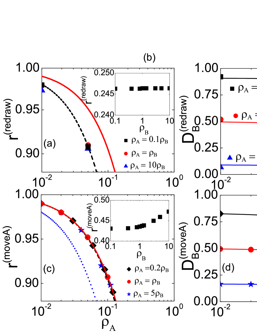
Figure 1: (Color online) Priority diffusion model on lattices. (a) The probability of a $B$ particle to be free for the redraw subprotocol, $r^{(redraw)}$, vs $\rho_{A}$. The dashed black line is for Eq. (III.2) and the red solid line is for $\exp(-\rho_{A})$. Inset: $r^{(redraw)}$ vs. $\rho_{B}$. (b) The diffusion coefficient of the low priority $B$ particles for the redraw subprotocol, $D_{B}^{(redraw)}$, vs $\rho_{A}$. Solid lines are for Eq. (8) after substituting Eq. (III.2). (c), (d) Same as (a) and (b), respectively, for the moveA subprotocol. In (c), the dotted blue line is for Eq. (III.2) for the moveA subprotocol, the solid red line is for $\exp(-\rho_{A})$, and the dashed black line is, for comparison, for Eq. (III.2) for the redraw subprotocol.

IV Priority diffusion in networks

We now turn to heterogeneous networks, where the degree $k$ varies from site to site. We focus on the particle protocol, and later discuss briefly the site protocol, which yields qualitatively similar results. We start with the fraction of empty sites of degree $k$, $f_{0}^{(k)}$. Consider a network with only one particle species and define a Markov chain on the states $\{0,1,2,...\}$ for the number of particles in a given site of degree $k$. The stationary probabilities are $f_{j}^{(k)}$. The chain has the transition probabilities:

$$P_{j,j-1}=\frac{j}{N\rho}\;;\quad P_{j,j+1}=\frac{k}{\left\langle k\right\rangle}\frac{1}{N}\;;$$ (12)

$P_{j,j}=1-P_{j,j-1}-P_{j,j+1}$ and all other probabilities are zero. $P_{j,j-1}$ is same as in Eq. (4). For a site to gain a particle, a neighboring site must first be chosen, and there are $k$ such sites. Since the neighbor is arrived at by following a random link, the probability that it has degree $k^{\prime}$ is $k^{\prime}P(k^{\prime})/\left\langle k\right\rangle$ (see, e.g., Generating ), and in that case, it will have, on average, $\rho k^{\prime}/\left\langle k\right\rangle$ particles (see below or, e.g., Rieger ). Since the particle is sent back to the original site with probability $1/k^{\prime}$, the overall probability for the original site to gain a particle is:

$$k\sum_{k^{\prime}=1}^{\infty}\left[\frac{k^{\prime}P(k^{\prime})}{\left\langle k\right\rangle}\cdot\frac{\frac{\rho k^{\prime}}{\left\langle k\right\rangle}}{N\rho}\cdot\frac{1}{k^{\prime}}\right]=\frac{k}{\left\langle k\right\rangle}\frac{1}{N}.$$ (13)

Solving for the stationary probabilities while keeping in mind that $\sum_{j}f_{j}^{(k)}=1$, one finds

$$f_{j}^{(k)}=f_{0}^{(k)}\frac{\left(\rho k/\left\langle k\right\rangle\right)^{j}}{j!}\;;\quad f_{0}^{(k)}=\exp\left({-\rho k/\left\langle k\right\rangle}\right).$$ (14)

Note that for regular networks, when all sites have the same degree, this reduces to Eq. (5), $f_{0}=e^{-\rho}$. The average number of particles in a site of degree $k$ is $\sum_{j=0}^{\infty}jf_{j}^{(k)}=\rho k/\left\langle k\right\rangle$, as expected.

When both species are involved, consider the redraw subprotocol where the $A$’s move independently of the $B$’s, and define that in one time step each particle has on average one moving attempt. At each time step, a $B$ particle in a node of degree $k$ has, on average, probability $\exp(-\rho_{A}k/\left\langle k\right\rangle)$ to jump out (Eq. (14)), since this is the probability of that site to have no $A$’s (assuming that the interaction between species is weak, as in lattices for large $\rho_{A}$ PRERC ). This results in an exponential distribution of waiting times (for a $B$ particle):

$$\psi_{k}(t)=\frac{1}{\tau_{k}}e^{-t/\tau_{k}},$$ (15)

with $\tau_{k}\equiv\exp(\rho_{A}k/\left\langle k\right\rangle)$. Simulation results confirming Eqs. (14) and (15) were shown in PRERC .

The exponentially long waiting time (in the degree $k$) means that in heterogeneous networks such as scale-free networks — where the degrees may span several orders of magnitude — the $B$ particles get mired in the hubs (high degree nodes). The problem is exacerbated by the fact that the $B$ particles are drawn to the hubs even in the absence of $A$’s: the presence of $A$’s only amplifies this tendency. In fact, the concentration of the $B$’s is proportional to $k\exp(\rho_{A}k/\left\langle k\right\rangle)$. To see this, denote by $n^{(B)}_{i}$ the number of $B$’s at node $i$. The probability of a $B$ to hop from node $i$ to a neighboring node $j$ in one time step is $p_{B}(i,j)=\exp(-\rho_{A}k_{i}/\left\langle k\right\rangle)\frac{1}{k_{i}}$, the product of the probability that node $i$ is free of $A$’s ( $\exp(-\rho_{A}k_{i}/\left\langle k\right\rangle)$) and the probability the particle is sent to node $j$ ($1/k_{i}$). In equilibrium, the number of $B$’s getting in and out of a node should be equal: $\sum_{j}n^{(B)}_{i}p_{B}(i,j)=\sum_{j}n^{(B)}_{j}p_{B}(j,i)$, and these equations are satisfied by $n^{(B)}_{i}\propto k_{i}\exp(\rho_{A}k_{i}/\left\langle k\right\rangle)$ (with the prefactor calculated from $\sum_{k}P(k)n^{(B)}(k)=\rho_{B}$). This is confirmed in Figure 2. Therefore, in large scale-free networks the $B$’s collect at the hubs and their diffusion is effectively halted.

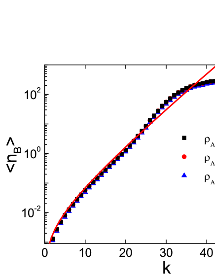
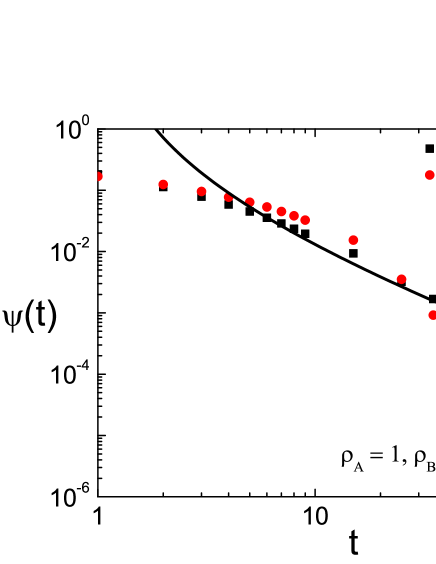
Figure 2: (Color online) The priority diffusion model on scale-free networks. (a) The average concentration of low priority particles, $n_{B}$, vs. the node degree $k$ for the redraw subprotocol in case of scale-free networks ($\gamma=3$, $k\geq 2$; generated as in MR ; symbols). Curves for different values of $\rho_{B}$ were normalized to collapse. The solid line stands for $\left\langle n_{B}\right\rangle\sim k\exp(\rho_{A}k/\left\langle k\right\rangle)$. (b) The distribution of waiting times $\psi(t)$ for $\rho_{A}=\rho_{B}=1$ for the case of the redraw subprotocol in scale-free networks (black squares) and ER networks with $\left\langle k\right\rangle=4$ (red circles). The black solid line represents Eq. (16), $\psi(t)\sim\frac{1}{\ln^{\gamma-1}t}$, further divided by $t$ to account for the fact that during our simulations, waiting times are sampled with probability inversely proportional to their duration (e.g., short waiting times are sampled more than long waiting times).

Using $n^{(B)}\sim k\exp(\rho_{A}k/\left\langle k\right\rangle)$, the probability of a random particle to reside in a node of degree $k$ is $G(k)\sim k\exp(\rho_{A}k/\left\langle k\right\rangle)P(k)$, where $P(k)$ is the degree distribution. We can now use $G(k)$ to find the waiting time distribution of a random particle, $\psi(t)$. Since $\psi_{k}(t)$ is relatively narrow, we replace it by a delta function $\psi_{k}(t)=\delta(t-\tau_{k})$, or $t(k)=\exp(\rho_{A}k/\left\langle k\right\rangle)$. For SF networks where $P(k)\sim k^{-\gamma}$, changing variables $\psi(t)dt=G(k)dk$ gives

$$\psi(t)\sim\frac{1}{\ln^{\gamma-1}t}.$$ (16)

The waiting time distribution is therefore broad, with some particles stalling for very long times. Eq. (16) for the waiting time distribution in SF networks is compared to simulations in Figure 2, as well as to the much narrower distribution in ER networks. Eq. (16) is expected to hold only up to time $\exp(\rho_{A}k_{\textrm{max}}/\left\langle k\right\rangle)$, where $k_{\text{max}}\sim N^{b}$, with $b=1/2$ for $2<\gamma<3$ and $b=\frac{1}{\gamma-1}$ for $\gamma\geq 3$ Boguna ; BurdaZ .

Analytical and simulation results have so far have assumed that the system is in equilibrium. Specifically, in each simulation, we used a “burn-in” period of $2000$ Monte Carlo steps. To investigate the dynamics of reaching equilibrium, we examined, in Figure 3, the rate at which the concentration profile $n(k)$ approaches its equilibrium form. This was quantified as the Sum of Squared Differences (SSD) between the profiles at consecutive time points:

$$\textrm{SSD}(t)=\sum_{k=2}^{k_{m}}{(\left\langle n_{t}(k)\right\rangle-\left\langle n_{t-1}(k)\right\rangle)^{2}},$$ (17)

where $\left\langle n_{t}(k)\right\rangle$ is the average particle concentration (either $A$’s or $B$’s) at nodes of degree $k$ at time $t$ and we set $k_{m}=50$. The results are shown in Figure 3 for two classes of initial conditions: (i) $A$’s and $B$’s are randomly distributed over all nodes (Figure 3) and (ii) all $A$’s are placed in the largest hub and all $B$’s are placed in the second largest hub (Figure 3). Uniform distribution has been tested and produces similar results as in Figure 3. In both cases, both species of particles reach equilibrium rapidly; but interestingly, $B$ particles equilibrate slower than $A$’s for uniform initial conditions and faster when initially placed on the hub. This happens because in equilibrium, most $B$’s are at the hubs, and therefore, if they start at the hub they will tend to remain in place. However, if the $B$’s are initially uniformly distributed, the priority constraints will slow them down on their way to reaching the hubs.

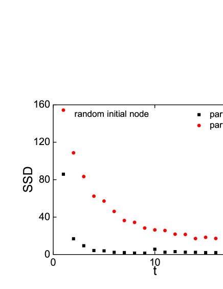
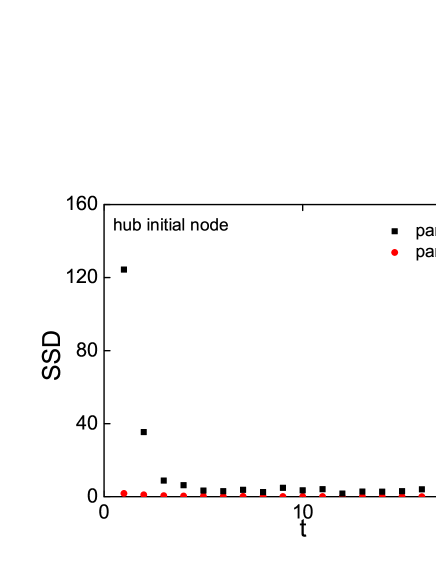
Figure 3: (Color online) The dynamics of approach to equilibrium in the priority diffusion model. In each panel, the Sum of Squared Differences (SSD) between the concentration profiles $\left\langle n(k)\right\rangle$ at successive time steps is plotted for both particle species. (a) $A$ and $B$ particles are randomly assigned an initial node. (b) All $A$ particles are initially placed in the largest hub and all $B$ particles are placed in the second largest hub. The overall concentrations were $\rho_{A}=1$ and $\rho_{B}=1$.

For the site protocol, the analytical approach presented in this section is not directly applicable, because transition probabilities for different degrees cannot be decoupled. Intuitively, however, it is clear that also for the site protocol the number of particles increases with the site degree. To see this, consider again a single species, and assume that the concentration $\rho$ is large enough that selected sites are never empty. For a given site, the probability to lose a particle is $1/N$ (the probability of the site to be selected). The probability to gain a particle is $\frac{1}{N}\sum_{j}\frac{1}{k_{j}}$, where the sum is over all $k$ neighbors of the site. Since the latter term scales as $k$, the number of gained particles is expected to increase with the site degree. With two species, that would again imply trapping of the low priority particles, just as in the particle protocol. This behavior is demonstrated in Figure 4.

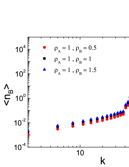
Figure 4: (Color online) The site protocol on scale-free networks. Plotted is the average concentration of the low priority particles, $n_{B}$, vs. the node degree $k$ for the site protocol on scale-free networks ($\gamma=3$, $k\geq 2$). The concentration increases with the node degree in a complex manner involving two phases (for which we have no theoretical arguments); the location of the transition point is in fact time-dependent (not shown).

To summarize so far, the combination of (i) heterogenous network structure, (ii) random walk, and (iii) strict priority policy leads to slowing down of the low priority particles. In the next section, we investigate strategies to enhance the mobility of the $B$ particles even under priority constraints.

V Strategies to avoid trapping of $B$’s

Given a heterogenous network structure, how can one implement a random walk with priorities, and yet guarantee the low priority particles are not halted?

V.1 moveA subprotocol

Recall the moveA subprotocol, in which $A$’s mobility is driven both by a selection of $A$’s and by a selection of arrested $B$’s. For this subprotocol, there is no trapping of the $B$’s since $A$’s do not aggregate at the hubs, but are rather rejected from them. Once an $A$ arrives into a node with many $B$’s, there is high probability for a $B$ to be chosen and push the $A$ outside the node. For this subprotocol, we numerically show that the probability of a site to be empty of $A$’s decays slower than exponentially in $k$, and that the average waiting time for a $B$ is short and almost independent of the degree (Figure 5).

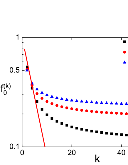
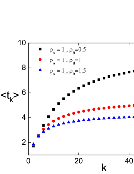
Figure 5: (Color online) The moveA protocol in networks. (a) The fraction of sites empty of $A$ particles, $f_{0}^{(k)}$, vs. the node degree $k$. The solid red line stands for $\exp(-\rho_{A}k/\left\langle k\right\rangle)$, the expression for the redraw protocol. (b) The average waiting time $\left\langle t_{k}\right\rangle$ vs. the node degree $k$. For large $k$, the waiting time is close to a constant.

V.2 Soft priorities

Consider a soft priority model, in which a $B$, when co-localized with $A$’s, has a small probability $\epsilon$ of leaving the site. As we show below, this results in enhanced diffusion of the $B$’s, even for networks.

Consider lattices first. An analytical solution can be derived as in the strict priority model (Section III.2), if the last line of Eq. (III.2) becomes:

$$P_{AB,B}^{(\rm{redraw})}=\frac{1}{N\rho_{S}}\;;\quad P_{AB,B}^{(\rm{moveA})}=\frac{2-\epsilon}{N\rho_{S}}\;;\$$

$$P_{AB,A}^{(\rm{redraw})}=\frac{\epsilon}{N\rho_{S}}\;;\quad P_{AB,A}^{(\rm{moveA})}=\frac{\epsilon}{N\rho_{S}}.$$ (18)

Using the last equation, the fraction of free $B$’s, up to first order, is:

$$r^{(\rm{redraw})}=1-\frac{2}{1+\epsilon}\rho_{A}+{\cal O}(\rho^{2})\;;$$

$$r^{(\rm{moveA})}=1-\rho_{A}+{\cal O}(\rho^{2}).$$ (19)

As in Section III.2, the first order solution can be substituted in the equations for the larger Markov chain that allows for two particles of the same species in a single site. Here, a $B$ will be free to move with probability $r+(1-r)\epsilon$. Solving the second order problem, we find:

$$r^{(\rm{redraw})}=1-\frac{2}{1+\epsilon}\rho_{A}+\frac{13+2\epsilon-3\epsilon^{2}}{2(1+\epsilon)^{2}(2+\epsilon)}\rho_{A}^{2}+{\cal O}(\rho^{3})\;;$$

$$r^{(\rm{moveA})}=1-\rho_{A}+\frac{3-\epsilon}{4}\rho_{A}^{2}+{\cal O}(\rho^{3}).$$ (20)

Note that Eq. (V.2) reduces to Eq. (III.2) in the case $\epsilon=0$, and to the series expansion of $e^{-\rho_{A}}$ for $\epsilon=1$ (no priorities, $A$’s and $B$’s are independent). Eq. (V.2) is compared to simulations in Figure 6. As for the case of strict priorities, $r$ is independent of $\rho_{B}$ and approaches $e^{-\rho_{A}}$ for large densities. The diffusion coefficients are:

$$D_{B}^{(\rm{redraw})}=\frac{\left[r+(1-r)\epsilon\right]\rho_{B}/\rho_{S}}{1-(1-r)(1-\epsilon)\rho_{B}/\rho_{S}}\;;$$

$$D_{B}^{(\rm{moveA})}=\left[r+(1-r)\epsilon\right]\rho_{B}/\rho_{S}.$$ (21)

Eq. (V.2) is compared to simulations in Figure 6. As expected, the diffusion of the $B$’s is always accelerated whenever $\epsilon>0$ for the redraw subprotocol. For the moveA subprotocol, $r$ decreases with increasing $\epsilon$, since $A$’s are rejected from sites that have $B$’s less often than in the $\epsilon=0$ case. However, at least for small $\rho_{A}$, the diffusion coefficient for the $B$’s increases with $\epsilon$: for small $\rho_{A}$, $r^{(\rm{moveA})}$ is very weakly dependent of $\epsilon$ (Eq. (V.2)), while $D_{B}^{(\rm{moveA})}$ increases linearly with $\epsilon$ (Eq. (V.2)).

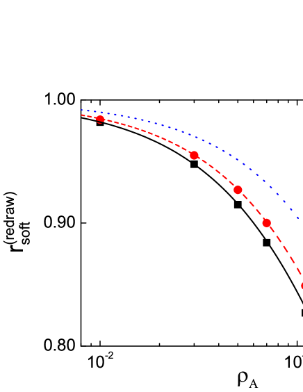
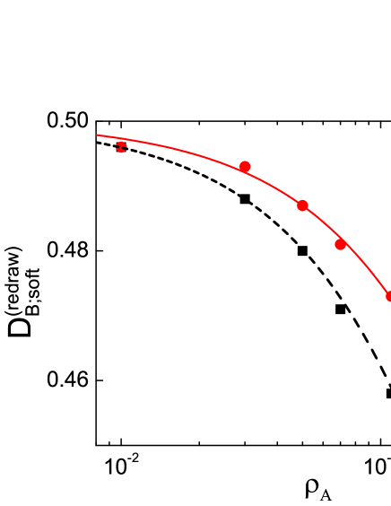
Figure 6: (Color online) Soft priorities on lattices. (a) The probability of a $B$ particle to be free in lattices with soft priorities, $r_{\textrm{soft}}^{(\textrm{redraw})}$, vs. $\rho_{A}$. The $B$ particle density is $\rho_{B}=\rho_{A}$. Solid black and dashed red lines are for Eq. (V.2); the dotted blue line stands for $\exp(-\rho_{A})$. (b) The diffusion coefficient of the $B$ particles, $D_{B;\textrm{soft}}^{(\textrm{redraw})}$, vs. $\rho_{A}$. Lines are for Eq. (V.2).

For networks, consider the particle protocol in the redraw version. $B$ particles can move if either (i) they are free, with probability $\exp(-\rho_{A}k/\left\langle k\right\rangle)$ or (ii) if they coexist with an $A$ but are allowed to jump, with probability $\epsilon\left[1-\exp(-\rho_{A}k/\left\langle k\right\rangle)\right]$. The average waiting time is the inverse of the hopping probability:

$$\tau_{k}=\frac{1}{\exp(-\rho_{A}k/\left\langle k\right\rangle)+\epsilon[1-\exp(-\rho_{A}k/\left\langle k\right\rangle)]}.$$ (22)

From Eq. (22), even for $k\rightarrow\infty$, $\tau_{k}\sim\epsilon^{-1}$ and thus diverges with $k$ only for $\epsilon=0$. This is confirmed in simulations (Figure 7). Therefore, even the slightest escape probability is sufficient to avoid the trapping of the low priority particles. In Figure 7, we plot the distribution of the low priority particles waiting times, $\psi_{\epsilon}(t)$, for different values of $\epsilon$. As expected, for $t\gg\epsilon^{-1}$ the decay is exponential.

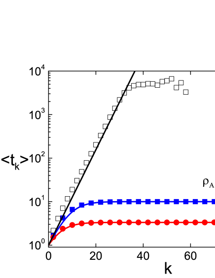
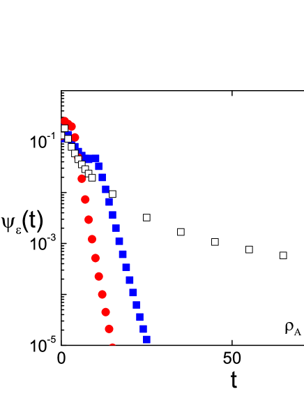
Figure 7: (Color online) Soft priorities on networks. (a) The average waiting time of $B$ particles, $\left\langle t_{k}\right\rangle$, vs. $k$, for the case of soft priorities redraw subprotocol (scale-free networks with $\gamma=3$ and $k\geq 2$; $\rho_{A}=\rho_{B}=1$). Solid lines are for Eq. (22). (b) The distribution of waiting times $\psi_{\epsilon}(t)$ for $\epsilon=0$ (open squares), $\epsilon=0.1$ (blue squares), and $\epsilon=0.3$ (red dots).

V.3 Avoiding hubs

One of the necessary conditions leading to the trapping of the $B$’s is the tendency of random walkers to concentrate at the hubs. This can be restrained if one assumes that each node is familiar with the degrees of its neighbors, and can thus avoid high degree nodes whenever possible. Consider the following model, where particles choose their next step according to the following rule Agata :

$$P_{ij}=\frac{k_{j}^{\alpha}}{\sum_{m}k_{m}^{\alpha}},$$ (23)

where $j$ is a neighbor of $i$ and the sum runs over all neighbors. Writing again a Markov chain for the number of particles per site (for a single species), the transition probabilities are:

$$P_{j,j-1}=\frac{j}{N\rho}\;;\quad P_{j,j+1}=\frac{k^{1+\alpha}}{\left\langle k^{1+\alpha}\right\rangle}\frac{1}{N}.$$ (24)

The probability to gain a particle was calculated as follows. Each neighboring node of the given site has probability $k^{\prime}P(k^{\prime})/\left\langle k\right\rangle$ to have degree $k^{\prime}$, and has on average $\rho k^{\prime 1+\alpha}/\left\langle k^{1+\alpha}\right\rangle$ particles Agata . The neighbor sends the particle to the given site with probability $k^{\alpha}/\frac{k^{\prime}\left\langle k^{1+\alpha}\right\rangle}{\left\langle k\right\rangle}$ Agata . Thus, the probability to gain a particle is:

$$k\sum_{k^{\prime}=1}^{\infty}\left[\frac{k^{\prime}P(k^{\prime})}{\left\langle k\right\rangle}\cdot\frac{\frac{\rho k^{\prime 1+\alpha}}{\left\langle k^{1+\alpha}\right\rangle}}{N\rho}\cdot\frac{k^{\alpha}}{\frac{k^{\prime}\left\langle k^{1+\alpha}\right\rangle}{\left\langle k\right\rangle}}\right]=\frac{1}{N}\frac{k^{1+\alpha}}{\left\langle k^{1+\alpha}\right\rangle}.$$ (25)

Following the same steps as before, this leads to:

$$f_{0}^{(k)}=\exp\left({-\frac{\rho k^{1+\alpha}}{\left\langle k^{1+\alpha}\right\rangle}}\right).$$ (26)

Eq. (26) is compared to simulations in Figure 8. For $\alpha=-1$, $f_{0}^{(k)}$ is independent of $k$ and we recover the lattice case. Whenever $\alpha>-1$, particles tend to aggregate at the hubs as before, leading again to trapping of low priority particles. When $\alpha<-1$, particles are attracted to the small nodes. However, since there are many small nodes, this does not lead to any further halting of the $B$’s. This is demonstrated in Figure 8, where the average waiting time of the $B$’s is plotted vs. $\alpha$. Requiring nodes to be aware of their neighbors’ degrees is reasonable in the context of communication networks, since this information can be attached to messages or exchanged between the nodes. Similar ideas were developed in bottleneck in the context of routing in communication networks. The drawback of the method is that by avoiding the hubs, it takes the particles more time to cover the network.

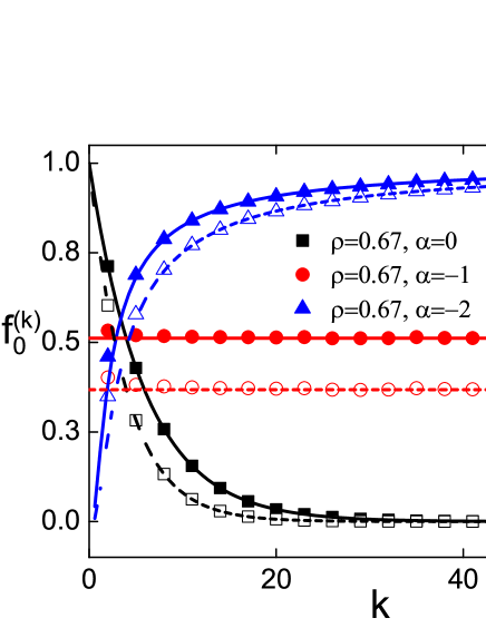
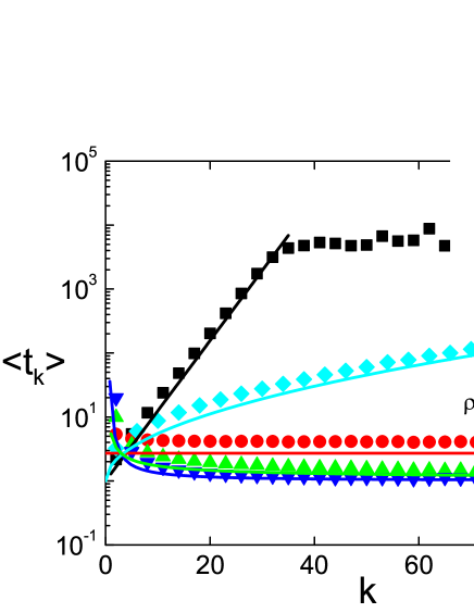
Figure 8: (Color online) The avoid hubs protocol. (a) The fraction of empty sites for one species, $f_{0}^{(k)}$, vs. the node degree $k$. Lines stand for Eq. (26). (b) The average waiting time of $B$ particles, $\left\langle t_{k}\right\rangle$, vs. $k$. Solid lines correspond to $\left\langle t_{k}\right\rangle=1/f_{0}^{(k)}=\exp\left(\rho k^{1+\alpha}/\left\langle k^{1+\alpha}\right\rangle\right)$.

V.4 Limited nodes capacity

In real communication applications, routers may be able to store only a limited amount of information. In our model, this constraint would translate to a limited number of particles in a node, such that particles cannot jump into nodes that have reached their capacity Capacity ; Chiense2011 . The analysis of such a model is complicated by the fact that particles are interacting even for a single species; for example, when the capacity is one particle per node, the particles are effectively fermions deMoura2005 ; SandersPRE2009 . We could nevertheless find an approximation to the fraction of empty sites. For concreteness, assume that each node has capacity $m(k)$ and that the single-species particle density is $\rho$. At each time step, a particle, selected at random, attempts to jump into one of its neighbors. However, if that neighbor is full, the jump is unsuccessful and the particle remains in place. Using again the Markov chain for the number of particles per site, and similarly to SandersPRE2009 , the transition probabilities for a node of degree $k$ are

$$P_{j,j-1}=\frac{j}{N\rho}\sum_{k^{\prime}=1}^{\infty}\frac{k^{\prime}P(k^{\prime})}{\left\langle k\right\rangle}\left(1-f_{m}^{(k^{\prime})}\right)\equiv\frac{jC}{N\rho}$$ (27)

$$P_{j,j+1}=k\sum_{k^{\prime}=1}^{\infty}\frac{k^{\prime}P(k^{\prime})}{\left\langle k\right\rangle}\frac{n(k^{\prime})}{N\rho}\frac{1}{k^{\prime}}=\frac{k}{N\left\langle k\right\rangle}~{}~{}(j<m).$$

The probability to lose a particle is $j/(N\rho)$, but then multiplied by the probability that the neighbor site is not full, $(1-f_{m})$. Since $f_{m}$ could be different for different degrees, we need to condition on the neighbor’s degree, but as the sum does not depend on either $k$ or $j$, it is a constant that depends on $\rho$ and $\left\langle k\right\rangle$ only and will be found later by computing the average density. In the second line, the probability to gain a particle is as in Sections IV and V.3, except that we denote the average number of particles in a site of degree $k^{\prime}$ as $n(k^{\prime})$. Using the relation $\sum_{k}P(k)n(k)=\rho$, the final transition probability is in fact as in the unconstrained Xcase. Using Eq. (27) and the normalization condition, it can be shown that the stationary probabilities satisfy (for $j=0,1,...,m(k)$)

$$f_{j}^{(k)}=\frac{\left(\frac{\rho k}{C\left\langle k\right\rangle}\right)^{j}/j!}{\sum_{j^{\prime}=0}^{m(k)}\left(\frac{\rho k}{C\left\langle k\right\rangle}\right)^{j^{\prime}}/j^{\prime}!}.$$ (28)

The constant $C$ is found by solving

$$\sum_{k=1}^{\infty}P(k)\frac{\sum_{j=1}^{m(k)}\left(\frac{\rho k}{C\left\langle k\right\rangle}\right)^{j}/(j-1)!}{\sum_{j=0}^{m(k)}\left(\frac{\rho k}{C\left\langle k\right\rangle}\right)^{j}/j!}=\rho,$$ (29)

an equation which also appeared in Capacity . Clearly, for $m(k)\rightarrow\infty$, $C\to 1$, and we reproduce the results of Section IV. Eq. (28) (for $j=0$) is compared to simulations in Figure 9.

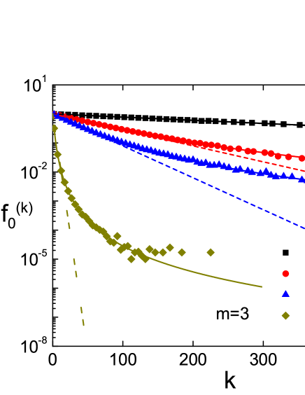
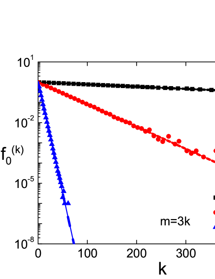
Figure 9: (Color online) Limited node capacity for one species. The fraction of empty sites for one species, $f_{0}^{(k)}$, vs. the node degree $k$ for (a) constant capacity $m=3$ and (b) variable capacity $m(k)=3k$. Full symbols present simulation results. Solid lines correspond to Eq. (28), while dashed lines correspond to the infinite capacity case, $f_{0}=\exp(-\rho k/\left\langle k\right\rangle)$.

With two species and the priority constraint, a reasonable choice for the capacity is $m(k)\propto k$, since nodes with larger degrees are usually more powerful and can handle more information. As shown in Capacity (see also Figure 9), the motion of the $A$ particles is not expected to be seriously affected due to the finite capacity. However, we have seen in Section IV that in the absence of capacity constraints, the $B$’s concentration grows as $k\exp(\rho_{A}k/\left\langle k\right\rangle)$. When finite capacity is imposed, $B$’s are not able to aggregate at the hubs as before, and their mobility is thus expected to be enhanced. This is demonstrated in Figure 10, where we plot the average concentration and the average waiting times for the $B$ particles.

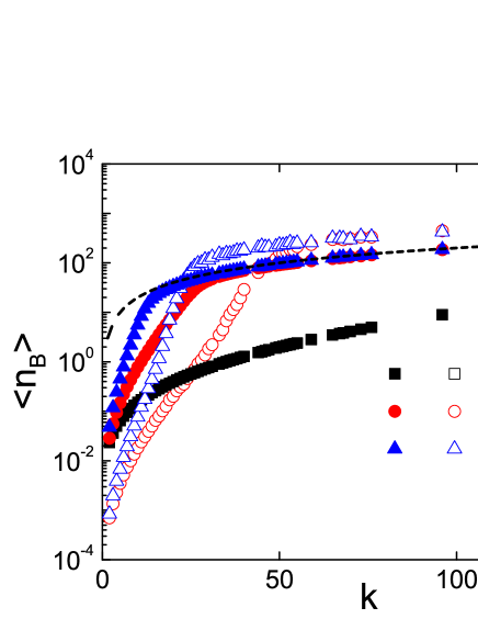
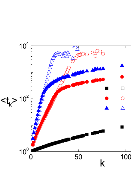
Figure 10: (Color online) The priority diffusion model with limited node capacity. (a) The average number of $B$ particles, $\left\langle n_{B}\right\rangle$, vs. $k$, for the case of limited node capacity with $m(k)=2k$. The black dashed line corresponds to the capacity, $n_{B}=m(k)$ (b) The average waiting time ,$\left\langle t_{k}\right\rangle$, vs. $k$. Full symbols are for limited capacity; empty symbols are for infinite capacity.

VI Summary

In summary, we introduced and analyzed a model of random walk with two species, $A$ and $B$, where the motion of one species ($A$) has precedence over that of the other. Our analytical results are summarized in Table 1. We obtained expressions for the diffusion coefficients in regular networks and lattices, for three possible particle selection protocols. In networks, we showed that the key quantity of the number of sites occupied by low-priority particles only decreases exponentially with the site degree. The consequence of this finding was an exponentially increasing concentration of the low priority particles in the hubs, followed by extremely long waiting times between consecutive hops. We used simulations to confirm this picture.

We then studied several strategies to improve the mobility of the low priority particles while maintaining the priority constraint. In the first strategy, we suggested that a selected $B$ that is unable to move will enforce hopping of a co-existing high-priority $A$. This results in the $A$’s being repelled out of sites with many $B$’s and prevention of the $B$’s trapping. The second strategy was to allow $B$ particles to jump ahead of the $A$’s with a small probability. We obtained the diffusion coefficients of the two species in lattices and showed that in networks, whenever the hopping probability is non-zero, the average waiting time of the $B$’s is finite even at the hubs. We then also considered modifying the nature of the random walk to preferential hopping into non-hub nodes and showed that this strategy distributes the particles more evenly, increasing the chances for a low priority particle to be free to move. Finally, we showed that limiting the queue size at each node can also prohibit the over-crowding of particles at the hubs. We note, however, that in the last two cases, while the waiting times of the low priority particles are shorter, the number of hops they would need to cover the network is expected to increase. We believe that our analytical and numerical results, for a wide variety of communication protocols and strategies, will be useful for communication network designers whenever protocols involve randomness and priority assignments.

Lattices	$f_{0}$	$r$	$D_{B}$
Site prot.	$\frac{1}{1+\rho}$		$\frac{\rho_{B}}{(1+\rho_{A})\rho_{S}}$
Redraw prot.	$e^{-\rho}$	$1-\frac{2}{1+\epsilon}\rho_{A}+\frac{13+2\epsilon-3\epsilon^{2}}{2(1+\epsilon)^{2}(2+\epsilon)}\rho_{A}^{2}+{\cal O}(\rho^{3})$	$\frac{\left[r+(1-r)\epsilon\right]\rho_{B}/\rho_{S}}{1-(1-r)(1-\epsilon)\rho_{B}/\rho_{S}}$
MoveA prot.		$1-\rho_{A}+\frac{3-\epsilon}{4}\rho_{A}^{2}+{\cal O}(\rho^{3})$	$\left[r+(1-r)\epsilon\right]\rho_{B}/\rho_{S}$
Networks	Normal	Avoid hubs	Limited capacity
$f_{0}$	$\exp\left(-\rho k/\left\langle k\right\rangle\right)$	$\exp\left(-\rho k^{1+\alpha}/\left\langle k^{1+\alpha}\right\rangle\right)$	$\left[\sum_{j=0}^{m(k)}\left(\frac{\rho k}{C\left\langle k\right\rangle}\right)^{j}/j!\right]^{-1}$
$\tau_{k}$	$\psi_{k}(t)$	$\psi(t)$	$n_{B}(k)$
$[f_{0}+\epsilon(1-f_{0})]^{-1}$	$\sim e^{-t/\tau_{k}}$	$\sim[\ln^{\gamma-1}t]^{-1}$	$\sim k\exp\left(\rho k/\left\langle k\right\rangle\right)$

Table 1: The analytical results derived in this paper. For lattices, three protocols were considered: a site selection protocol and a particle selection protocol with either redraw or moveA subprotocols when a $B$ is selected in a site in which $A$s are also present. We calculated the fraction of empty sites, $f_{0}$, for one species of density $\rho$ as well as the diffusion coefficient of the $B$s, $D_{B}$, for two species of densities $\rho_{A}$ and $\rho_{B}$ ($\rho_{S}=\rho_{A}+\rho_{B}$). For the particle protocols, we calculated a low density approximation for $r$, the probability of a $B$ particle to be free. $\epsilon$ is a “soft priority” probability to move a $B$ particle in the presence of $A$s. For networks, the first two rows show the fraction of empty sites, $f_{0}$, either for normal diffusion, or when hubs are avoided, or when the capacity at the nodes is limited. $k$ is the degree; $\left\langle k\right\rangle$ is the average degree; $\alpha$ is the degree-preference exponent (sites are visited with probability proportional to $k^{\alpha}$); $m(k)$ is the capacity of a node of degree $k$; and $C$ is a normalization coefficient calculated from Eq. (29). The final two rows provide additional quantities for networks: $\tau_{k}$ is the average time spent in a node of degree $k$ (here, soft priorities are also included); $\psi_{k}(t)$ is the distribution of waiting times of $B$ particles at sites of degree $k$; $\psi(t)$ is the distribution of all waiting times; and $n_{B}(k)$ is the average number of $B$ particles at a node of degree $k$.

Appendix: Shortest path routing

In this appendix, we show that the statistical properties of traffic in homogeneous networks with shortest path routing resemble, for some networks, those of a random walk. Consider an all-pairs communication model, where packets are sent from all nodes to all other nodes along shortest paths. Denote the source node as $i$ and the destination as $j$. At each intermediate node $m$ along the path, the packet must be sent to the neighbor of $m$ closest to $j$. If the network is homogeneous, we expect the next node on the path to be, with roughly equal probability, any of the neighbors of $m$, similar to a random walk. To test this, we numerically calculated the fraction of messages routed through each link (which is also the betweeness centrality centrality ) in our model networks. We compared this quantity, which we call $R$, to $1/k$ ($k$ is the degree of the node from where the message was sent), the probability to route through the link in the case of a random walk. We found that indeed, for the relatively homogeneous regular and ER networks, the probability of routing through a link is narrowly distributed around $1/k$ (Figure 11). For the heterogeneous SF networks, the distribution of routing probabilities is wider, since most shortest paths visit specifically the hubs. Thus, as long as the network is homogeneous, our model is expected to describe, at least qualitatively, also the traffic resulting from shortest path routing with priorities.

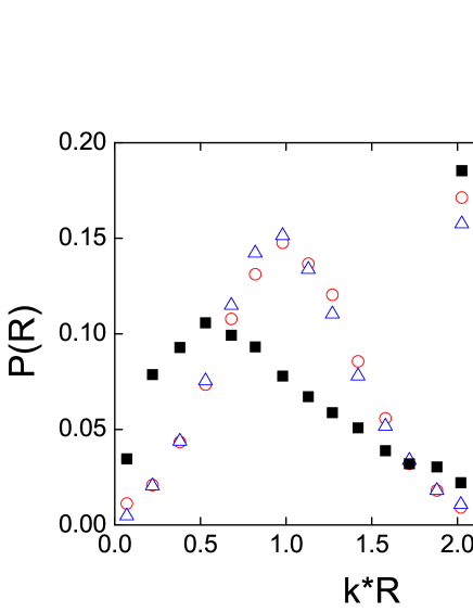
Figure 11: (Color online) $P(R)$, The distribution of $R$, the fraction of messages that are routed through a link emerging from a node of degree $k$. Results are averages over 5 realizations for the case of $k=5$. Black squares are for scale-free networks ($\gamma=3,k\geq 2$), open red circles are for ER with $\left\langle k\right\rangle=3$, and open blue triangles are for ER with $\left\langle k\right\rangle=5$. Note that the x-axis is scaled by $1/k$. The distribution is narrowly centered around $1/k$ for ER networks, but not for SF networks.

References

- [1] R. Albert and A.-L. Barabási. Rev. Mod. Phys., 74:47–94, 2002.
- [2] R. Pastor-Satorras and A. Vespignani. Structure and Evolution of the Internet: A Statistical Physics Approach. Cambridge University Press, Cambridge, 2004.
- [3] S. N. Dorogovtsev and J. F. F. Mendes. Evolution of Networks: From Biological Nets to the Internet and WWW. Oxford University Press, Oxford, 2003.
- [4] M. E. J. Newman. The structure and function of complex networks. SIAM Review, 45:167–256, 2003.
- [5] W.-X Wang, B.-H. Wang, C.-Y. Yin, Y.-B. Xie, and T. Zhou. Traffic dynamics based on local routing protocol on a scale-free network. Phys. Rev. E, 73:026111, 2006.
- [6] W.-X. Wang, C.-Y. Yin, G. Yan, and B.-H. Wang. Integrating local static and dynamic information for routing traffic. Phys. Rev. E, 74:016101, 2006.
- [7] W. Huang and T. W. Chow. Investigation of both local and global topological ingredients on transport efficiency in scale-free networks. Chaos, 19:043124, 2009.
- [8] D. De Martino, L. Dall’Asta, G. Bianconi, and M. Marsili. Congestion phenomena on complex networks. Phys. Rev. E, 79:015101, 2009.
- [9] S. Meloni and J. Gómez-Gardeñes. Local empathy provides global minimization of congestion in communication networks. Phys. Rev. E, 82:056105, 2010.
- [10] R. Cohen and S. Havlin. Complex Networks: Structure, Robustness and Function. Cambridge University Press, Cambridge, 2010.
- [11] M. E. J. Newman. Networks: An Introduction. Oxford University Press, New York, 2010.
- [12] X. Ling, M.-B. Hu, R. Jiang, and Q.-S. Wu. Global dynamic routing for scale-free networks. Phys. Rev. E, 81:016113, 2010.
- [13] C. Avin and C. Brito. Efficient and robust query processing in dynamic environments using random walk techniques. In Proc. of the third international symposium on Information processing in sensor networks, pages 277–286, 2004.
- [14] D. Braginsky and D. Estrin. Rumor routing algorthim for sensor networks. In Proc. of the 1st ACM Int. workshop on Wireless sensor networks and applications, pages 22–31. ACM Press, 2002.
- [15] Z. Bar-Yossef, R. Friedman, and G. Kliot. Rawms -: random walk based lightweight membership service for wireless ad hoc network. In MobiHoc ’06: Proceedings of the seventh ACM international symposium on Mobile ad hoc networking and computing, pages 238–249, New-York, NY, USA, 2006. ACM Press.
- [16] S. Dolev, E. Schiller, and J. Welch. Random walk for self-stabilizing group communication in ad-hoc networks. In Proceedings of the 21st IEEE Symposium on Reliable Distributed Systems (SRDS’02), pages 70–79. IEEE Computer Society, 2002.
- [17] C. Gkantsidis, M. Mihail, and A. Saberi. Random walks in peer-to-peer networks. In Proc. 23 Annual Joint Conference of the IEEE Computer and Communications Societies (INFO-COM), 2004.
- [18] J. F. Kurose and K. W. Ross. Computer Networking: A Top-Down Approach Featuring the Internet. Addison Wesley, third edition, 2004.
- [19] A. S. Tanenbaum. Computer Networks. Prentice Hall PTR, fourth edition, 2002.
- [20] K. Kim, B. Khang, and D. Kim. Jamming transition in traffic flow under the priority queuing protocol. EPL, 86:58002, 2009.
- [21] M. Maragakis, S. Carmi, D. ben Avraham, S. Havlin, and P. Argyrakis. Priority diffusion model in lattices and complex networks. Phys. Rev. E, 77:020103(R), 2008.
- [22] M. R. Evans and T. Hanney. Phase transition in two species zero-range process. J. Phys. A: Math. Gen., 36:L441–L447, 2003.
- [23] G. M. Schutz. Critical phenomena and universal dynamics in one-dimensional driven diffusive systems with two species of particles. J. Phys. A: Math. Gen., 36:R339 –R379, 2003.
- [24] L. Bogacz, Z. Burda, W. Janke, and B. Waclaw. Free zero-range processes on networks. Proceedings of SPIE, 6601:66010V, 2007.
- [25] B. Waclaw, Z. Burda, and W. Janke. Power laws in zero-range processes on random networks. Eur. Phys. J. B, 65:565–570, 2008.
- [26] P. Erdős and A. Rényi. Publ. Math. (Debreccen)., 6:290–297, 1959.
- [27] B. Bollobás. Random Graphs. Academic Press, Orlando, 1985.
- [28] S. Carmi, S. Havlin, S. Kirkpatrick, Y. Shavitt, and E. Shir. A model of internet topology using -shell decomposition. Proc. Natl. Acad. Sci. USA, 104:11150–11154, 2007.
- [29] M. E. J. Newman, S. H. Strogatz, and D. J. Watts. Random graphs with arbitrary degree distributions and their applications. Phys. Rev. E, 64:026118, 2001.
- [30] J. D. Noh and H. Rieger. Phys. Rev. Lett., 92:118701, 2004.
- [31] M. Molloy and B. Reed. The size of the giant component of a random graph with a given degree sequence. Combinatorics, 7:295–305, 1998.
- [32] M. Boguñá, R. Pastor-Satorras, and A. Vespignani. Cut-offs and finite size effects in scale-free networks. Eur.Phys.J.B., 38:205–209, 2004.
- [33] Z. Burda and A. Krzywicki. Uncorrelated random networks. Phys. Rev. E, 67(046118), 2003.
- [34] A. Fronczak and P. Fronczak. Biased random walks on complex networks: the role of local navigation rules. Phys. Rev. E, 80:016107, 2009.
- [35] S. Sreenivasan, R. Cohen, E. Lopez, Z. Toroczkai, and H. E. Stanley. Communication bottlenecks in scale-free networks. Phys. Rev. E, 75:036105, 2007.
- [36] R. Germano and A. P. S. de Moura. Traffic of particles in complex networks. Phys. Rev. E, 74:036117, 2006.
- [37] Q.-K. Meng and J.-Y. Zhu. Constrained traffic of particles on complex networks. Chin. Phys. Lett., 28:078901, 2011.
- [38] A. P. S. de Moura. Fermi-dirac statistics and traffic in complex networks. Phys. Rev. E, 71:066114, 2005.
- [39] D. P. Sanders. Exact encounter times for many random walkers on regular and complex networks. Phys. Rev. E, 80:036119, 2009.
- [40] U. Brandes. A faster algorithm for betweenness centrality. Journal of Mathematical Sociology, 25:163–177, 2001.