$N$-body insights into the Milky Way’s X-shape

Abstract

Using simulations of box/peanut- (B/P-) shaped bulges, we explore the nature of the X-shape of the Milky Way’s bulge. An X-shape can be associated with a B/P-shaped bulge driven by a bar. By comparing in detail the simulations and the observations we show that the principal kinematic imprint of the X-shape is a minimum in the difference between the near and far side mean line-of-sight velocity along the minor axis. This minimum occurs at around $|b|=4\degr$, which is close to the lower limit at which the X-shape can be detected. No coherent signature of an X-shape can be found in Galactocentric azimuthal velocities, vertical velocities, or any of the dispersions. After scaling our simulations, we find that a best fit to the Bulge Radial Velocity Assay data leads to a bar angle of $15\degr$. We also explore a purely geometric method for determining the distance to the Galactic Centre by tracing the arms of the X-shape. We find that we are able to determine this ill-known distance to an accuracy of about 5% with sufficiently accurate distance measurements for the red clump stars in the arms.

1 Introduction

About one-quarter of the stars in the local Universe are hosted by the bulges of disc galaxies (Persic & Salucci, 1992; Fukugita et al., 1998). Bulges can be either ‘classical’ or ‘pseudo’ bulges, with mixed types also possible (e.g. Erwin et al., 2003; Debattista et al., 2005; Athanassoula, 2005; Nowak et al., 2010). Classical bulges form via merging of sub-galactic clumps, satellites and clusters (Eggen et al., 1962; Tremaine et al., 1975; Searle & Zinn, 1978; Kauffmann et al., 1993; Baugh et al., 1996; van den Bosch, 1998; Hopkins et al., 2010). On the other hand, pseudo bulges form via secular evolution of the disc (Combes & Sanders, 1981; Combes et al., 1990; Raha et al., 1991; Norman et al., 1996; Courteau et al., 1996; Bureau & Freeman, 1999; Debattista et al., 2004; Athanassoula, 2005; Drory & Fisher, 2007; Kormendy & Kennicutt, 2004). Understanding the mix of bulges present in the Universe therefore represents an important step towards understanding galaxy formation.

When viewed edge-on, roughly $45\%$ of galaxies host box/peanut- (B/P-) shaped bulges (Burbidge & Burbidge, 1959; Shaw, 1987; Lütticke et al., 2000; Laurikainen et al., 2011), which are associated with bars (Kuijken & Merrifield, 1995; Bureau & Freeman, 1999; Chung & Bureau, 2004). B/P-shaped bulges can also be recognized photometrically at moderate inclinations (Quillen et al., 1997; Bettoni & Galletta, 1994; Erwin & Debattista, 2013) and, kinematically, even in face-on galaxies (Debattista et al., 2005; Méndez-Abreu et al., 2008). B/P-shapes are supported by ’banana’ and ’anti-banana’ orbits, which have been extensively studied (Pfenniger & Friedli, 1991; Combes et al., 1990; Pfenniger, 1984, 1985; Patsis et al., 2002). They arise from vertically unstable x1 orbits, even when the non-axisymmetry driving them is weak (Patsis et al., 2002).

The origin of the Milky Way’s bulge remains an issue of disagreement. On the one hand the Milky Way’s bulge is part of a bar (Dwek et al., 1995), and is rapidly rotating (Shen et al. 2010, but see also Saha et al. 2012). On the other hand, the bulge consists largely of old (Ortolani et al., 1995; Kuijken & Rich, 2002; Valenti et al., 2003; Zoccali et al., 2003; Clarkson et al., 2008, 2011), $\alpha$-enhanced stars (McWilliam, 1997). It is now well-established that the Milky Way hosts a bar (Dwek et al., 1995; Binney et al., 1997; Bissantz & Gerhard, 2002; López-Corredoira et al., 2005; Vanhollebeke et al., 2009). The first signs of a near/far asymmetry in the bulge of the Milky Way were found by Rangwala et al. (2009), who noted differences in velocities in Baade’s window and in two other fields ($l=\pm 5\degr$, $b=-3.5\degr$). Soon thereafter, both Nataf et al. (2010) and McWilliam & Zoccali (2010) independently identified a split in the red clump (RC) towards the Galactic Centre. Nataf et al. (2010) used 267 fields taken from the OGLE-III survey (Udalski et al., 2008) at $-10\degr<l<10\degr$ and $2\degr<|b|<7\degr$. They found two distinct RCs towards many of these lines-of-sight. They also noticed that both RCs are equally populated, and that these trends are found in the Northern and Southern hemispheres. McWilliam & Zoccali (2010) used four independent photometric data sets, Two Micron All Sky Survey (2MASS) (Skrutskie et al., 2006), WFI and SOFI photometry (Zoccali et al., 2003) and OGLE (Udalski et al., 2002) maps, to show that the double RC is real and is present at $b\ga 4\degr$ in all the data sets. Their analysis of 2MASS observations also suggested a three-dimensional X-shape. De Propris et al. (2011), using data from the Galaxy and Mass Assembly (GAMA) Survey (Driver et al., 2011) for a field at ($l$,$b$)$=(0\degr,-8\degr)$, found no discernible difference between the near and the far sides in both radial velocity and radial velocity dispersion. Saito et al. (2011) used 2MASS (Skrutskie et al., 2006) data at $|l|\leq 8.5\degr$ and $3.5\degr\leq|b|\leq 8.5\degr$ to construct a 3D density map of the X-shaped bulge. They found that the X-shape is oriented at an angle of 20° to the line-of-sight. They also found that the arms merge at $|b|\leq 4\degr$, implying that the X-shape is absent in Baade’s Window. Ness et al. (2012), using the ARGOS survey in three fields ($l$ = 0° $b=-5\degr,-7.5\degr,-10\degr$), also found an X-shape. They found a difference in the line-of-sight velocities of the two clumps which can be reproduced qualitatively by an $N$-body model of a buckled bar from Athanassoula (2003). Another comparison of a numerical model to the Milky Way was provided by Li & Shen (2012). When viewed like the Milky Way, their model contains an X-shaped structure similar to the one in the Galaxy which they show arises from the buckled bar. At higher latitudes, $(l,b)=(0\degr,-10\degr)$, Uttenthaler et al. (2012) measured radial velocities for the near and far RC and found that the two distributions are indistinguishable from each other. Recently, Vasquez et al. (2013) obtained full space velocities for RC stars in the near and far arms of the X-shape at $(l,b)=(0\degr,-6\degr)$. They find a difference in the mean line-of-sight velocities but none in the mean vertical velocities of these stars. They compared their observations to an $N$-body model from Debattista et al. (2005) (which we also use in this paper), finding qualitative agreement between them.

This paper uses $N$-body simulations of barred galaxies to explore the effect of B/P-bulge shapes of various strengths and at different orientations on the observed kinematics of stars. We also study whether it is possible to measure the distance to the Galactic Centre using the X-shape.

2 Simulations

We use the sample of high force and mass resolution barred galaxy simulations described in Debattista et al. (2005), who used these simulations to explore the kinematic signature of face-on B/P bulges. In units where $R_{\rm d}=M_{\rm d}=G=1$ (where $R_{\rm d}$ and $M_{\rm d}$ are the disc’s exponential scale-length and mass, respectively, and $G$ is the gravitational constant), which gives a unit of time $(R_{\rm d}^{3}/GM_{\rm d})^{1/2}$, the values for the disk$+$halo parameters are set such that the rotation curves were always approximately flat to large radii. Debattista et al. (2005) provides full details of the parameters of the different models. In scaling from simulation units to size in kiloparsecs ($L$) and velocities in km s^-1 ($V$), the mass of the disc becomes

$$M=\frac{LV^{2}}{4.3\times 10^{-6}\mathrm{~{}kpc~{}M_{\odot}^{-1}~{}(km~{}s^{-1})^{2}}}$$ (1)

For example, Debattista et al. (2006) suggested a scaling with $L=2.5$ kpc and $V=200$ km s^-1, so that the stellar mass $M=2.3\times 10^{10}M_{\odot}$.

These simulations span a range of bulge, disc and halo properties resulting in B/P shapes of varying strength. The main simulations we consider from that paper are R1, B3 and R5. Comparison with models R2, R6, and B2 from the same paper are presented in the Appendix. Models in the R series had no initial bulges, while models B2 and B3 hosted classical bulges from the start. Models R1 and R2 both form strong B/P shapes via the usual buckling instability. The B/P shape in model R2 extends to a larger fraction of the bar size than in model R1. Model R5 instead forms a quite weak B/P shape, while model R6 never formed one. Both model B2 and B3 formed B/P shapes. In the former case, this is somewhat masked by the presence of a classical bulge, but in model B3 the B/P shape is readily apparent despite the presence of a classical bulge. Further details, including face-on and edge-on views, of all the models can be found in Debattista et al. (2005). An animation of the formation and evolution of the B/P shape in model R1 is presented in Debattista et al. (2006) (where this model is referred to as model L2). Images of the three models considered here, R1, B3 and R5, are shown in Fig. 1, for reference. These images adopt our preferred scaling, which is described below. It is worth noting in Fig. 1 that model R1 is not symmetric about the mid-plane, having a more prominent B/P-shape at $z>0$ than at $z<0$. The main part of the paper will concentrate in-depth on models R1 and B3 which host the clearest X-shapes. Model R5 is an example of a weak B/P shape.

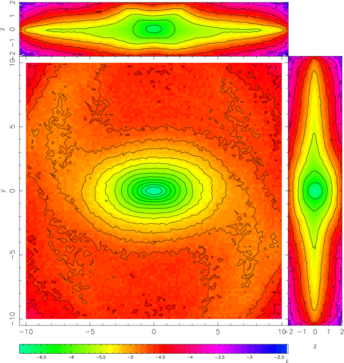
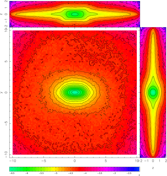
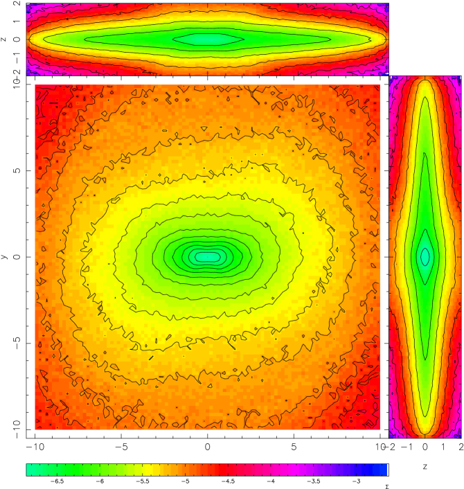
Figure 1: Three orthogonal projections of the density of models R1 (top), B3 (middle) and R5 (bottom) as seen from outside the system. In each case the bar has been rotated on to the $x$-axis.

We generally compute velocities in our models as observer-centred without correcting for the peculiar motion of the observer relative to the local standard of rest, unless otherwise noted. However, we also consider azimuthal velocities (V_ϕ) which are always in the galactocentric reference frame.

3 Scaling the simulations

The size scaling is chosen to match the size of the bar in the Milky Way (3.43 kpc Robin et al. 2012). Fig. 1 shows three models scaled to this size with the bar rotated into the $x$-axis. Additionally, we use the bar as a measure of the near and far sides of the bulge, choosing anything beyond the centre of the galaxy, up to half a bar length, as the far side, and from the centre of the galaxy to half a bar length towards the observer as the near side. This is done to better refine our study to just the regions where the X-shape is expected to lie. The scalings differ from model to model, with $L=2.4,3.0$ and $3.5$ kpc in models R1, B3 and R5, respectively.

In order to be able to compare our models to the Milky Way, we will also have to choose what angle the model will be viewed from, as well as the multiplicative scaling factor from simulation velocity units to km s^-1. We used BRAVA (Bulge Radial Velocity Assay, Kunder et al., 2012) data of radial velocities from the fields at $-10\degr\leq l\leq 10\degr$ at $b=-$6°, $-$8° and $-10\degr\leq l\leq 22\degr$ at $b=-$4°. We match by minimizing $\chi^{2}$ between the means and standard deviations of the line-of-sight velocities in the BRAVA data and in our model data. We correct for the solar motion using the solar velocities of Schönrich (2012) and assume a Sun-Galactic Centre distance of 8 kpc. We convolve our models with the selection function of M-giant stars along the various lines of sight of the BRAVA data, including the 3D dust extinction maps from Marshall et al. (2006). In order to compute the selection functions, we generate a large sample of stars in each direction located in a solid angle of $2.1\degr\times 2.1\degr$ around the field centre and with apparent $K$-band magnitude between 8.2 and 9.25. Then we compute the probability for a star to be selected by the survey as a function of distance in each direction by evaluating how many stars have been selected in the observed sample among all the stars present at a given distance regardless of their magnitude. The two selection functions with peaks nearest ($D\simeq 5$ kpc) and furthest ($D\simeq 6$ kpc) from the Sun are shown in Fig. 2. The full-width at half-maximum of the selection functions are generally in the range $4-5$ kpc.

Figure 2: Examples of selection functions for BRAVA stars. We show only two lines-of-sight, with the nearest, ($l,b$) = ($-9\degr,-4\degr$), (dashed line) and the furthest, ($l,b$) = ($-6\degr,-8\degr$), (solid line) peak. The selection functions for the other fields have similar profiles and fall between these two.

3.1 Choosing the angle of the bar

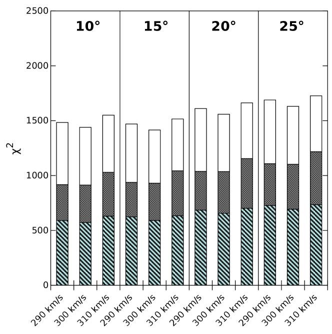
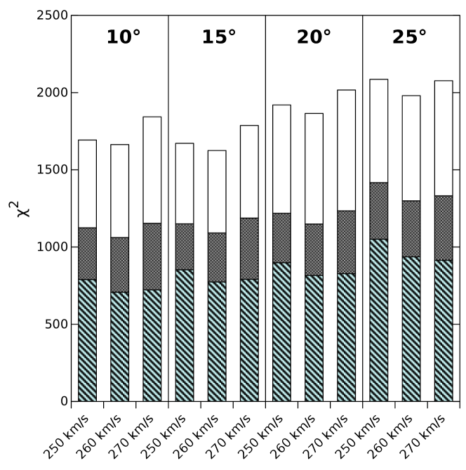
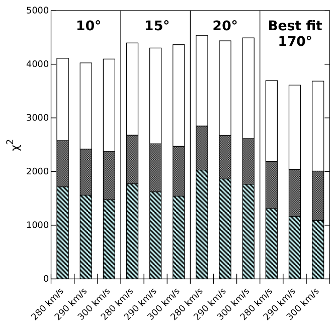
Figure 3: $\chi^{2}$ of fits to the BRAVA data for models R1 (top), B3 (middle) and R5 (bottom) varying the velocity scaling, $V$, and the angle of the bar in the simulation. The shaded areas, from bottom to top, show the individual $\chi^{2}$-values for the BRAVA fields at $b$= $-$4°, $-$6° and $-$8°. The angles, 10°, 15°, 20° and 25°  are separated by vertical lines. For model R5 we show the $\chi^{2}$-values for 10°, 15°, 20° and the best fit at 170°. Note the difference in vertical scale in the bottom panel compared with the others.

The bar angle to the line joining the Sun to the galactic centre was chosen by minimizing the $\chi^{2}$ for angles between 10°and 50° in steps of 1°. Both models R1 and B3 resulted in a $\chi^{2}$ minimum at a bar angle of 15°. Fig. 3 shows how the change in bar angle affects the value of $\chi^{2}$. We use $\Delta\chi^{2}=\chi^{2}-\min(\chi^{2})$, where $\min(\chi^{2})$ is the minimum value of $\chi^{2}$, to estimate the probable $1\sigma$ confidence interval on the angle as $\Delta\chi^{2}<\sqrt{2N_{obs}}$, where $N_{obs}$ is the number of observables used in the comparison (van den Bosch & van de Ven, 2009). We obtain $\pm 5\degr$ for model R1 and $\pm 10\degr$ for model B3. Model R5 instead produces a best fit at 170°. However, the $\chi^{2}$ of the best fit is more than twice that of R1 or B3, and is almost triple for an angle of 15°. For consistency, we will always show model R5 at a bar angle of 15°. Fig. 3 shows a breakdown of the $\chi^{2}$ by fields at different $b$. For both model R1 and B3, the largest contribution to $\chi^{2}$ comes from the fields closest to the mid-plane, $b=-4\degr$, while the $b=-6\degr$ fields contribute the least. This is not the case for model R5 however, which has a contribution from the $b=-8\degr$ fields comparable, or larger than, the ones at $b=-4\degr$.

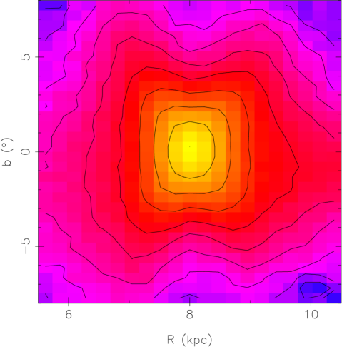
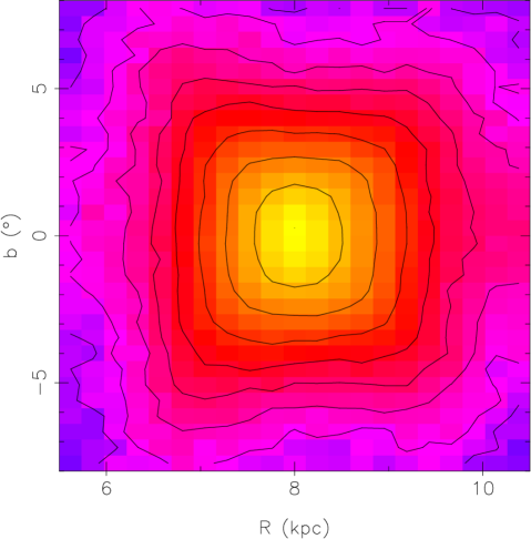
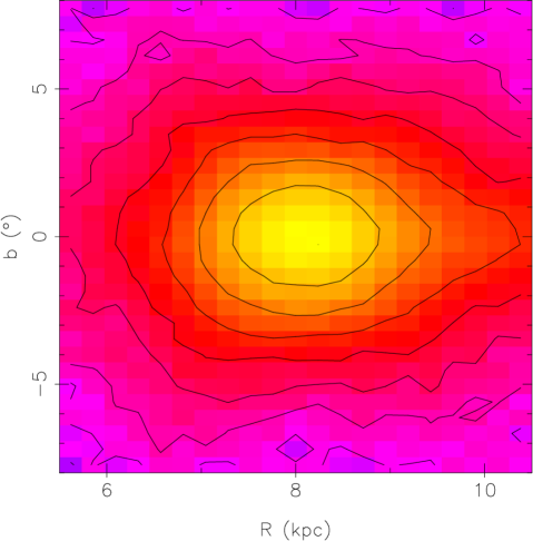
Figure 4: Density of models R1 (top), B3 (middle) and R5 (bottom) in the $l=0\degr$ plane. The plot shows the density as a function of latitude and distance from the observer. This mimics the projection in fig. 4 of Saito et al. (2011). The bar angle is set to $15\degr$ in each case.

The models in Fig. 4 are shown in the $(R,b)$ plane at $l=0\degr$, as in Saito et al. (2011). The mock-observations have not been corrected for the volume effect, instead including all particles along a given line-of-sight, since the observations we compare with are themselves not corrected for the volume effect. The X-shape in model R1 exhibits an asymmetry across $b=0\degr$, arising from its intrinsic asymmetry across the mid-plane. Its arms can be traced down to about $3\degr$, becoming boxy at lower $b$. The X-shape in the bulge of model B3 is much less readily apparent, though it clearly has a boxy shape. Model R5 has a weakly boxy shape in Fig. 1, but no evidence of an X-shape in Fig. 4.

3.2 Choosing the velocity scale

After fitting the bar angle, we choose the velocity scale, $V$. Although choosing the velocity scale and bar angle are intricately linked, we verified that there was no difference which was chosen first. The best velocity scale for R1 was $V=299$ km s^-1, which differs from the one we used in Vasquez et al. (2013), 250 km s^-1, for which we fitted only a single BRAVA field. For B3, the $\chi^{2}$ minimum is at $V=257$ km s^-1. For R5, the best velocity scale for a bar angle of 15° is $V=291$ km s^-1.

4 Comparison of simulations to observations

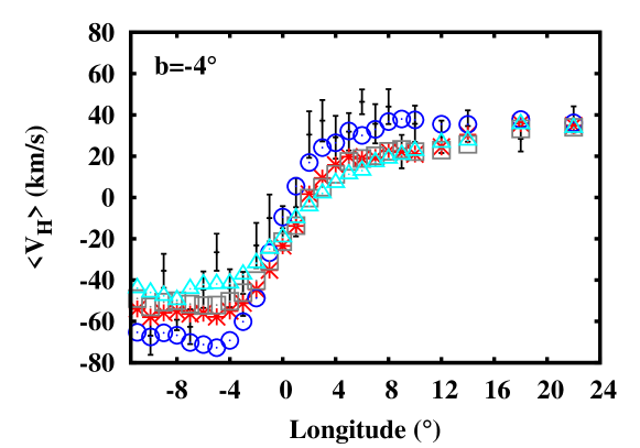
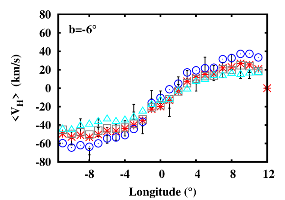
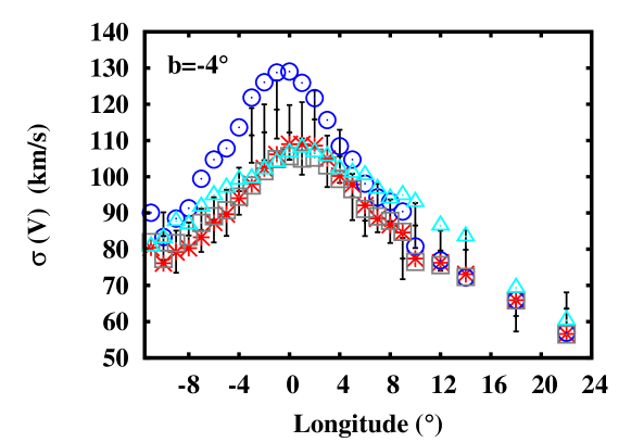
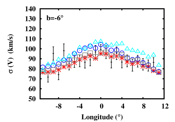
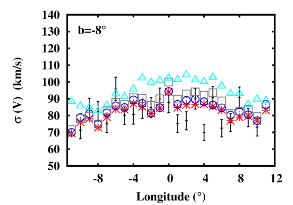
Figure 5: Mean heliocentric velocities and velocity dispersions for BRAVA fields along strips of $b=-4\degr$, $-6\degr$ and $-8\degr$. Data: points with error bars; models : R1: grey squares, B3: red stars, R5: cyan triangles, Fux: blue circles. The model data have been obtained using the BGM, sampling velocities from the $N$-body models.

In comparing the kinematics predicted by $N$-body simulations to real observational data it should be remembered that observations are generally not based on a volume-limited sample but rather on a magnitude-limited sample. Sometimes, additional selections are included as well (e.g. reddened or de-reddened colours, proper motion-selected, temperature-selected, gravity-selected, etc.). In the previous section, when comparing the $N$-body simulations to BRAVA data, we estimated the selection function in distance from the luminosity function of M giants and a 3-D extinction model. We assumed that the observational data trace a distance interval without additional selection biases. This was suitable for computing the scaling of the $N$-body simulations. In the present section we investigate whether the kinematics of the particles in the $N$-body simulations are comparable to real stellar kinematics, once all selection biases, such as the varying fraction of M-giants with distance, are taken into account. The population synthesis approach is well-suited for this purpose.

4.1 Population synthesis model comparison with BRAVA data

We simulate the BRAVA sample with the M-giant distribution in the Besançon Galaxy Model (BGM) and compare the heliocentric radial velocity distributions in different fields. We apply the kinematics of the $N$-body simulations to the stars in the bar component of the BGM. The kinematics are computed using the mean and dispersion of the particle velocities on the three axes in boxes 250 pc wide in Cartesian $(x,y,z)$ coordinates covering the whole bar. Then, for each M-giant star drawn from the BGM bar population, we randomly apply velocities from the Gaussian distribution with the mean and dispersion of the position of the star, which, to first order, should reproduce the velocity field of the bar in the $N$-body simulation. Notice that this approximation may not be valid in rare regions where the distribution is very skewed. Moreover, in some locations where the number of particles in the $N$-body simulation is small, the velocity is taken to be undefined since otherwise the assumed kinematics are noisy. This can be remedied by applying some form of smoothing to the model velocities. In the regions dominated by the bar, the number of particles in the simulation is sufficient for a reliable value of the mean and the dispersion of the velocities so we have not had to smooth the velocity field in this experiment.

To generate the stellar populations we use the version of the BGM described in Robin et al. (2012). This includes five components: a thin disc, a thick disc, a stellar halo, a bar and a bulge. For simulating the BRAVA sample, we select M giants in the apparent magnitude range $8.2<K_{s}<9.25$, as explained in Kunder et al. (2012), assuming the distribution of the extinction along the line-of-sight from the Marshall et al. (2006) 3D maps.

The statistics (mean and standard deviation) of the heliocentric radial velocity of BRAVA fields along latitudes $-$4°, $-$6°and $-$8° (from Kunder et al. 2012) are compared with the output of the BGM, as described above, in Fig. 5. We also compare with the kinematics drawn from the earlier model of Fux (1999). BRAVA data are shown with error bars (given by Poisson uncertainties). The model simulations cover slightly larger angular areas in order to minimize Poisson noise.

Globally, two of our $N$-body models, R1 and B3, perform well, indeed better than the Fux model, while R5 fails to properly fit the observations. At $b=-4\degr$ models R1, B3 and R5 appear slightly shifted in velocity at $2\degr\leq l\leq 11\degr$. In this region, the Fux model performs better. But at negative longitudes, R1, B3 and R5 are significantly better than the Fux model, which encounters problems, as already noted by Howard et al. (2009). R1, B3 and R5 are slightly different at negative longitudes, but the difference (about 5 $-$ 10 km s^-1) is small compared with the uncertainty in the BRAVA data. The velocity dispersions from R1, B3 and R5 are good approximations for almost all longitudes, given the uncertainties. They differ from each other only in the central region and only by a few km s^-1. At $b=-$8° the models do not differ much within the uncertainties of the data, except for model R5, where the velocity dispersions are systematically too high. At $b=-$6°, the differences between the Fux model, R1, and B3 are more noticeable. The Fux model rotates too fast and has too large velocity dispersion at negative longitudes. Model R5 fits the BRAVA data more poorly, because of slower rotation and an even higher velocity dispersion than the Fux model.

This test confirms that any selection biases are likely to be small. Overall models R1 and B3 are good approximations to the observed kinematics over a large range of longitudes and latitudes in the bulge region. Model R1 gives a slightly better fit. However, the BRAVA data are unable to distinguish between models R1 and B3, because the sample in each direction is small and M giants cannot distinguish the near and far sides. Hence, further tests using RC giants, especially in regions where the clump is double, will be performed in the near future.

4.2 Model comparison to other observations

We next compare our two main B/P-shaped bulge simulations (R1 and B3) with kinematic data from the literature. The results of this comparison are compiled in Table 1.

Table 1: Comparison of observational values for the differences between mean velocities and velocity dispersions of the near and far sides of the bulge and the same quantities in our models. Velocities are in km s^-1. For the models, we consider $b<0\degr$ and $b>0\degr$ measurements separately, the latter indicated by $(+b)$ at the top of each column.

Reference	$l$	$b$	$|\Delta\overline{V}|$	$\Delta\sigma_{V}$	R1		(+$b$)	(+$b$)	B3		(+$b$)	(+$b$)
					$|\Delta\overline{V}|$	$\Delta\sigma_{V}$	$|\Delta\overline{V}|$	$\Delta\sigma_{V}$	$|\Delta\overline{V}|$	$\Delta\sigma_{V}$	$|\Delta\overline{V}|$	$\Delta\sigma_{V}$
Rangwala et al. (2009)	5.5°	$-$3.5°	40 $\pm$ 11		14		22		26		24
	$-5\degr$	$-3.5\degr$	32 $\pm$ 12		16		28		27		26
De Propris et al. (2011)	$0\degr$	$-8\degr$	10 $\pm$ 14	4 $\pm$ 14	9	7	8	9	22	6	15	4
Ness et al. (2012)	$0\degr$	$-5\degr$	30 $\pm$ 12		10		14		28		28
	$0\degr$	$-7.5\degr$ and $-10\degr$	7 $\pm$ 9		5		13		17		17
Vasquez et al. (2013)	$0\degr$	$-6\degr$	21 $\pm$ 14	10 $\pm$ 10	11	6	12	6	28	5	23	1

Compared to the line-of-sight velocities in Rangwala et al. (2009), we find similar differences, although the one at negative $l$ does not fit as well as the field at positive $l$; however the field at positive instead of negative $b$ fits the data much better. Compared to the data of De Propris et al. (2011), we find that R1 fits their data better, showing very little difference in the line-of-sight velocities and line-of-sight velocity dispersions of the near and far sides. Thus this is not an ideal location to search for the kinematic signature of the X-shaped bulge. For the Ness et al. (2012) data we find a better fit to the lower latitude field of B3, but a worse fit for the combined two higher latitude fields, where the difference in observations is small.

We use a different value for the local standard of rest than we did in Vasquez et al. (2013), adopting ($U,V,W$)_⊙ = (14, 12, 6) km s^-1 and V_c = 238 km s^-1 from Schönrich (2012) to derive heliocentric velocities. For the observations in $(l,b)=(0\degr,-6\degr)$, the differences between the velocities of the near and far sides for $U,V$ and $W$ are, respectively, 5 $\pm$ 14, 23 $\pm$ 19 and 13 $\pm$ 16 km s^-1 for the mean and 6 $\pm$ 10, 18 $\pm$ 13 and 11 $\pm$ 12 km s^-1 for the dispersions. For R1, the differences of means are 2, 1 and 1 km s^-1, while the differences in dispersions are 9, 5 and 3 km s^-1. For B3 the differences are 3, 2 and 3 km s^-1 for the means and 7, 4 and 3 km s^-1 for the dispersions. The differences are substantially lower, but well within the errors as well as consistent with the previous estimates for differences of R1 in Vasquez et al. (2013).

5 The kinematic imprint of the X-shape

5.1 Mapping near-/far side kinematic differences across the bulge

We next examine how the kinematics of the near and far sides of the bulge differ across the whole bulge region. We consider the square region defined by $|l|,|b|<10\degr$ aiming to uncover the kinematic signature of the B/P-shaped bulge. Given an axisymmetric system, the kinematic differences between the near and far sides of the bulge should be featureless. We calculate maps of the difference between the near and far side mean and dispersion of line-of-sight, galactocentric azimuthal and vertical velocities.

Fig. 6 shows the differences for the line-of-sight velocities and dispersions. It is immediately apparent that there is a qualitative difference between models R1 and B3, both with X-shapes, and model R5 without. In model R5, the contours of the difference in mean velocities are more or less lines of constant $l$. In models R1 and B3 instead contours corresponding to the largest differences in mean velocity cross the $l=0\degr$ plane at $|b|\simeq 3\degr-4\degr$. In model R1 this leads to the striking result that the velocity difference is larger at $b>0\degr$, where we showed above that the B/P-shape is also stronger, than at $b<0\degr$. The inescapable conclusion is that this difference is a kinematic imprint of the X-shape. The difference between the velocities is generally negative (in our frame a positive velocity corresponds to a motion away from the Sun). The line-of-sight velocity dispersion has positive differences at positive $l$. In all three models the differences in both the mean and dispersion of line-of-sight velocities have a peak near ($l,b$)= ($5\degr,0\degr$).

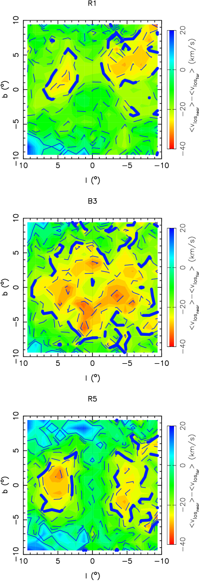
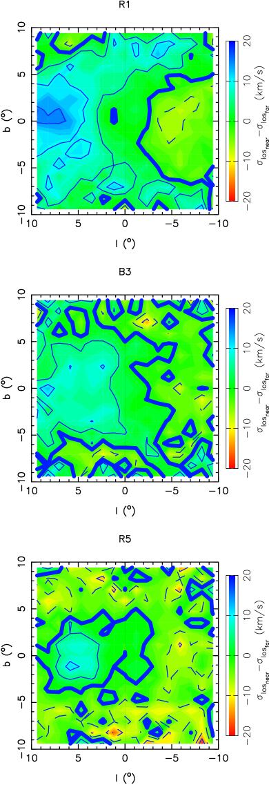
Figure 6: Differences between near and far side line-of-sight mean velocity (left panels) and near and far side line-of-sight velocity dispersion (right panels). Contours are spaced by 5 km s^-1 and the bold contour marks 0 km s^-1. Dashed contours show negative values, while solid contours show positive values.

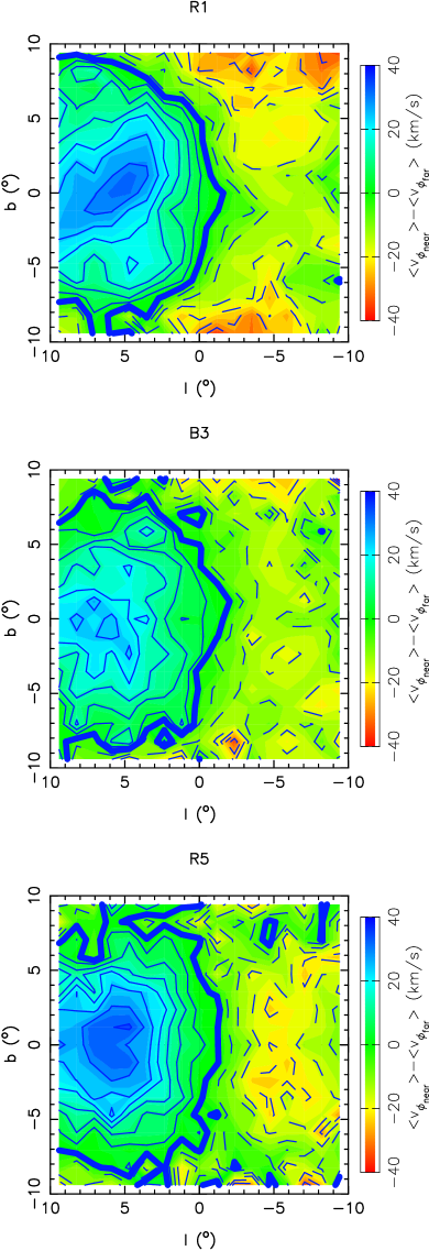
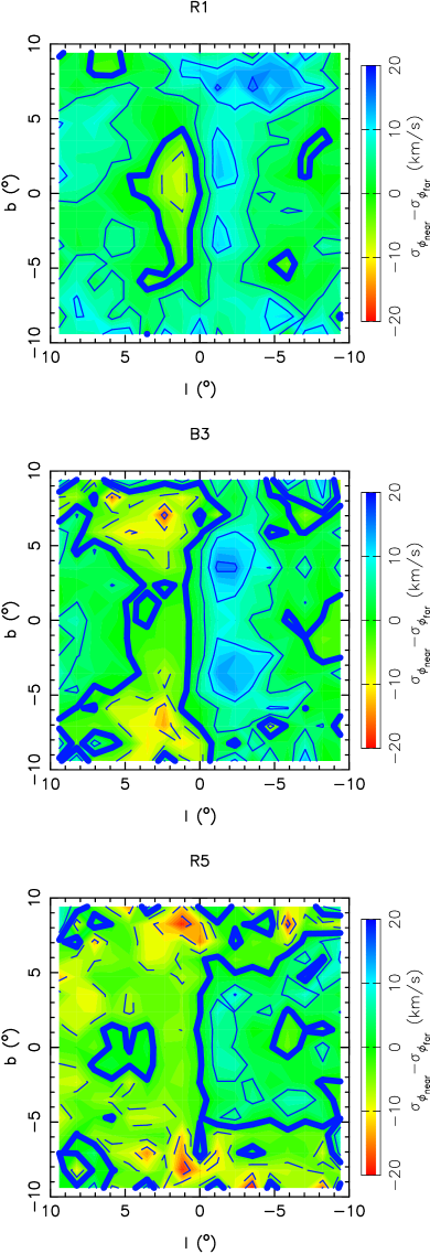
Figure 7: Differences between near and far side mean galactocentric azimuthal velocity (left panels) and near and far side galactocentric azimuthal velocity dispersion (right panels). Contours are spaced by 5 km s^-1 and the bold contour marks 0 km s^-1. Dashed contours show negative values, while solid contours show positive values.

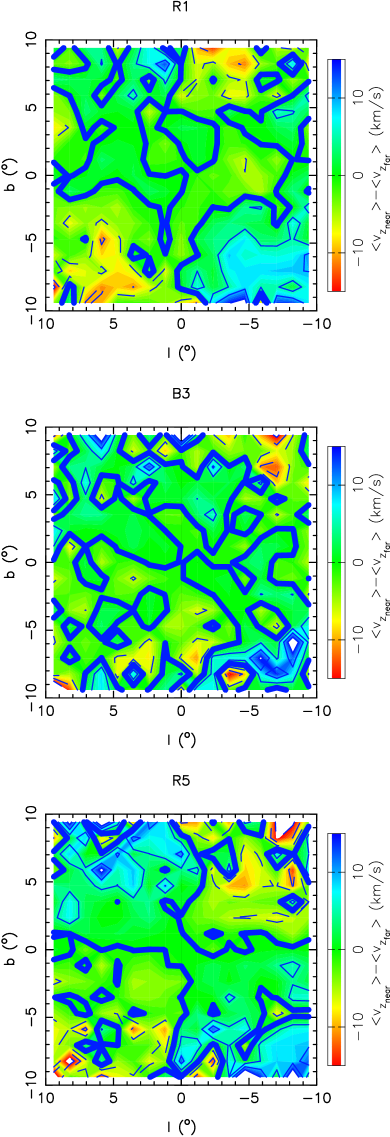
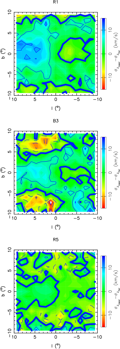
Figure 8: Differences between near and far side mean vertical velocity (left panels) and near and far side vertical velocity dispersion (right panels). Contours are spaced by 5 km s^-1 and the bold contour marks 0 km s^-1. Dashed contours show negative values, while solid contours show positive values.

For galactocentric azimuthal velocities (Fig. 7), there is a difference between the near and far sides evident in the average velocity (left panels) and in the velocity dispersion (right panels), for all three models. The largest differences in the average velocity are close to where the near side of the bar is located, around ($l,b$) = ($6\degr,\pm 1\degr$). The largest differences in the azimuthal velocity dispersion can be found around ($l,b$) = ($-2\degr,9\degr$) for R1 and ($l,b$) = ($3\degr,\pm 8\degr$) and ($l,b$) = ($-2\degr,\pm 4\degr$) for B3. The differences are small for R5, centred at ($l,b$) = ($-2\degr,0\degr$). However, qualitatively there is no difference between models R1 and B3 with an X-shape, and model R5 without, in either the difference of mean velocities or the difference of dispersions.

Vertical velocities (Fig. 8) again show no coherent difference between the near and far sides. There are small (5-10 km s^-1) positive differences in vertical velocity dispersion near $b$ = 0° at positive $l$. There are a few anomalous regions in vertical velocity dispersion for B3, located at $8\degr<l<0\degr,b=\pm 8\degr$, which appear also in the azimuthal velocity dispersion.

Overall, the result of this analysis is that the strongest imprint of an X-shape is in the near/far side difference in mean line-of-sight velocities. The galactocentric tangential mean velocities and vertical velocities do not betray the presence of an X-shape, nor do any of the velocity dispersions to any significant extent.

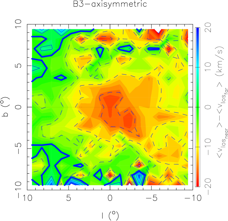
Figure 9: Near/far side differences in mean $V_{los}$ in model B3 which has been rendered axisymmetric by azimuthally shuffling all particles.

Finally, we use model B3, which had one of the strongest near/far-side asymmetries in $V_{los}$, to demonstrate that the asymmetry is a signature of the X-shape by removing it by axisymmetrising the model. The resulting map of $\Delta V_{los}$, which is shown in Fig. 9, has a minimum at $(l,b)=(0\degr,0\degr)$ and decreases more or less monotonically with $|b|$, in stark contrast with B3 when it is not axisymmetrised. This adds further weight to our interpretation of a minimum in $\Delta V_{los}$ off $b=0\degr$ as being the kinematic signature of an X-shape.

5.2 Line-of-sight velocities at $l=0\degr$

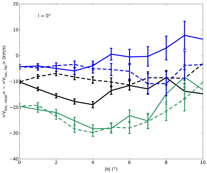
Figure 10: Near/far side differences in mean $V_{los}$ in the $l=0\degr$ plane for models R1 (black lines), B3 (green lines) and R5 (blue lines). Solid (dashed) lines show $b>0\degr$ ($b<0\degr$).

Fig. 10 plots the near$-$far side difference in mean $V_{los}$. Errors in $\Delta V_{los}$ are calculated by taking the combination in quadrature of the errors of the means for each field on the near and far side. In all models this difference is negative throughout, presumably in part because the volumes probed are different. Additionally, in model B3 and in $b>0\degr$ of model R1 a very clear minimum across $|b|$ at $l=0\degr$ exists which is caused by the X-shape. No comparable minimum is present at $b<0\degr$ in model R1 (dashed black line). Nor is there a similar minimum in model R5.

We now examine V_los in the field $(l,b)=(0\degr,-6\degr)$ of Vasquez et al. (2013), and consider how bar angles of 15°, 25° and 35° affect the distribution. The sub-panels of Fig. 11 each have separate distributions, for the near (dashed lines) and far sides (full lines). In this figure, we also show the distribution of the observed bright (red line) and faint (blue line) red clump stars from Vasquez et al. (2013). The means of the distributions of $V_{los}$ differ significantly, with the far side having slightly more positive velocities (in our convention positive $V_{los}$ velocities correspond to stars moving away from the observer), while the near side stays at zero, or has negative velocities. This is seen in the observations as well as the models. As the bar angle increases, the negative velocity of the near side becomes more prominent. The differences between the two means of the radial velocity distribution are 11.6, 25.9 and 34.1 km s^-1 for angles of 15°, 25° and 35°, respectively, for R1, and 28.4, 33.5 and 35.2 km s^-1 for the same angles in B3. Velocity dispersions differ by less than 10 km s^-1, for both models, with the difference becoming smaller at larger bar angles. Thus the near/far sides asymmetry provides a sensitive probe of the bar angle. Despite the qualitative agreement between the observational data and the models, it is difficult to interpret quantitatively. There are two reasons for this: (i) the significant Poisson noise in the data and (ii) the mismatch in the definition of the near/far sides between the models and the bright/faint RCs in Vasquez et al. (2013). Therefore, the bar angle cannot be derived reliably from this comparison. Conversely, the kinematic imprint of an X-shape is not masked by any plausible value of the bar angle. Rather surprisingly, while the density maps at $l=0\degr$ of R1 and B3 in Fig. 4 are relatively different, the two models have qualitatively similar distributions of $V_{los}$.

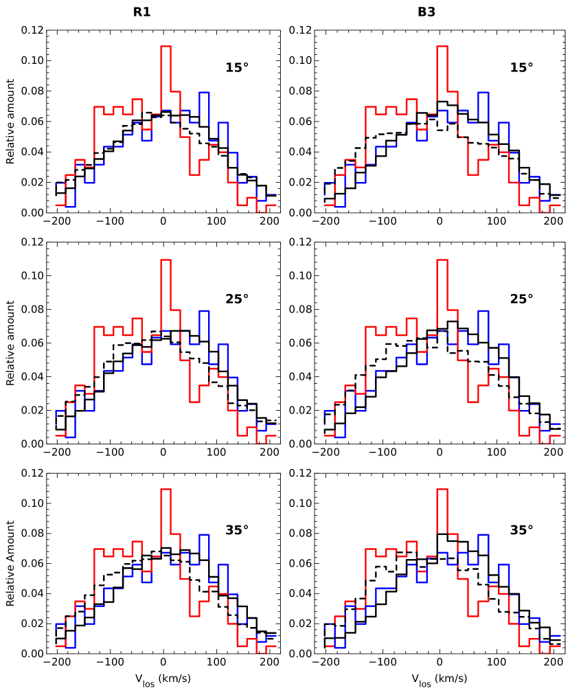
Figure 11: Distributions of line-of-sight velocities for the near (dashed lines) and far sides (solid lines) of the scaled models at bar angles, 15° (top), 25° (middle) and 35° (bottom). Distributions are for the field at $(l,b)=(0\degr,-6\degr)$. The solid red and blue lines correspond to, respectively, the observed velocities from the bright RC and the faint RC and are identical in all six panels. The left column is for model R1 while the right one is for model B3. All distributions have been normalized to unit area.

5.3 Bulge versus disc near/far side kinematic differences

We now consider the different behaviours of the disc and classical bulge in model B3. Fig. 12 presents the density distribution at $l=0\degr$ separately for the two components. A very prominent X-shape is present in the disc component, whereas the bulge has a boxy shape. Fig. 13 compares the disc (left panels) and bulge (right panels) differences in mean velocities; the most striking result is that the kinematic signature of the X-shape, the minimum in the line-of-sight velocity along $l=0\degr$, appears only in the disc not the bulge. The remaining kinematics, including the near/far side differences in velocity dispersions (Fig. 14), merely show the effect of a higher rotation and lower dispersion in the disc relative to the bulge.

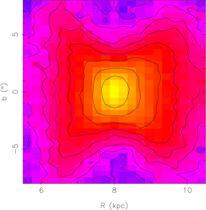
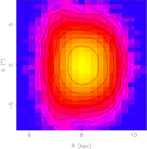
Figure 12: Density of the disc (left) and classical bulge (right) at $l=0\degr$ in model B3.

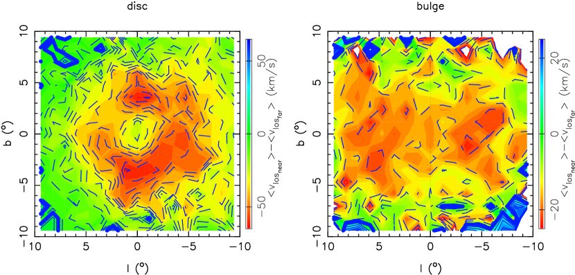
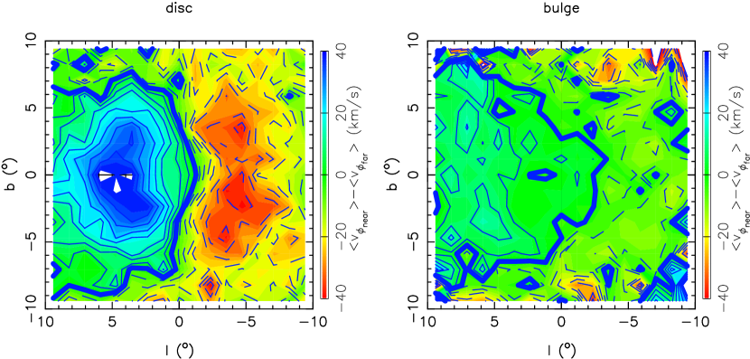
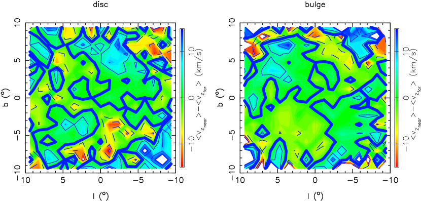
Figure 13: Differences between near and far side velocities for the disc (left) and classical bulge (right) components of model B3. The top, middle and bottom rows show differences in the line-of-sight, tangential ($\phi$) and vertical ($z$) directions. Contours are spaced by 5 km s^-1 and the bold contour marks 0 km s^-1. Dashed contours show negative values, while solid contours show positive values.

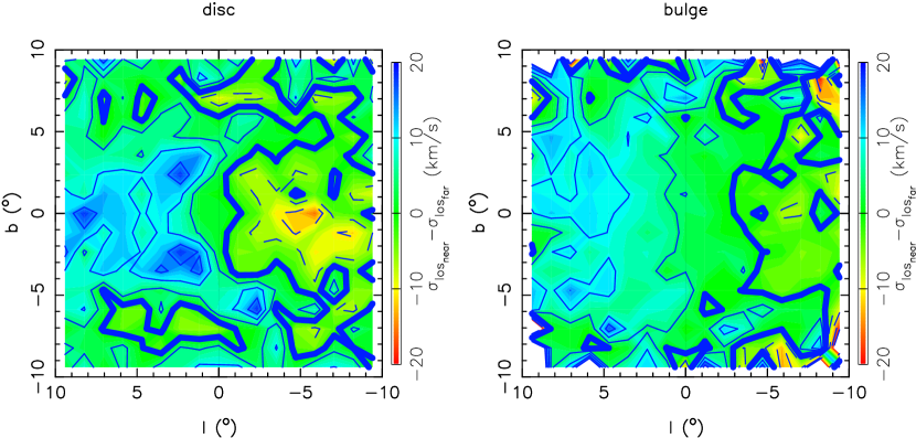
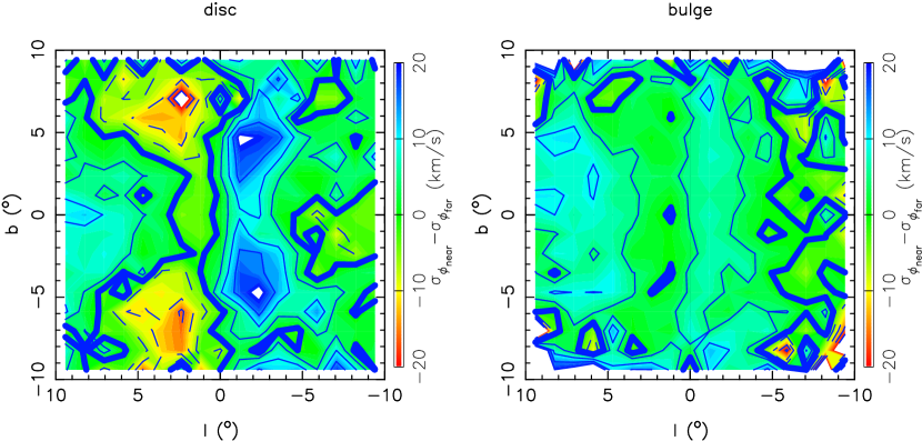
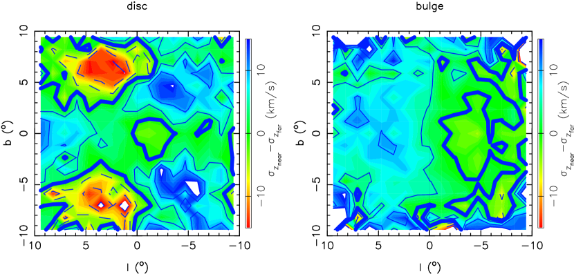
Figure 14: Differences between near and far side velocity dispersions for the disc (left) and classical bulge (right) components of model B3. The top, middle and bottom rows show differences in the line-of-sight, tangential ($\phi$) and vertical ($z$) directions. Contours are spaced by 5 km s^-1 and the bold contour marks 0 km s^-1. Dashed contours show negative values, while solid contours show positive values.

5.4 Gas $+$ star formation simulation

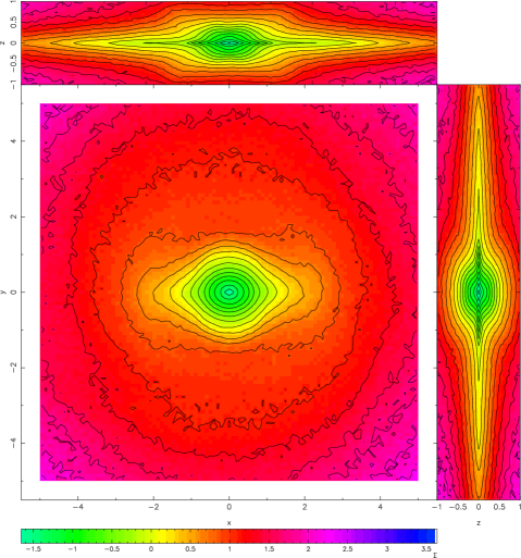
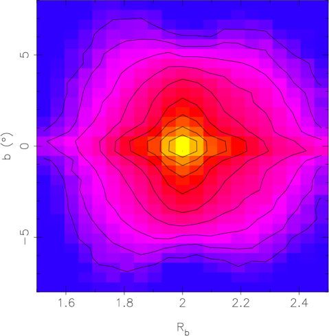
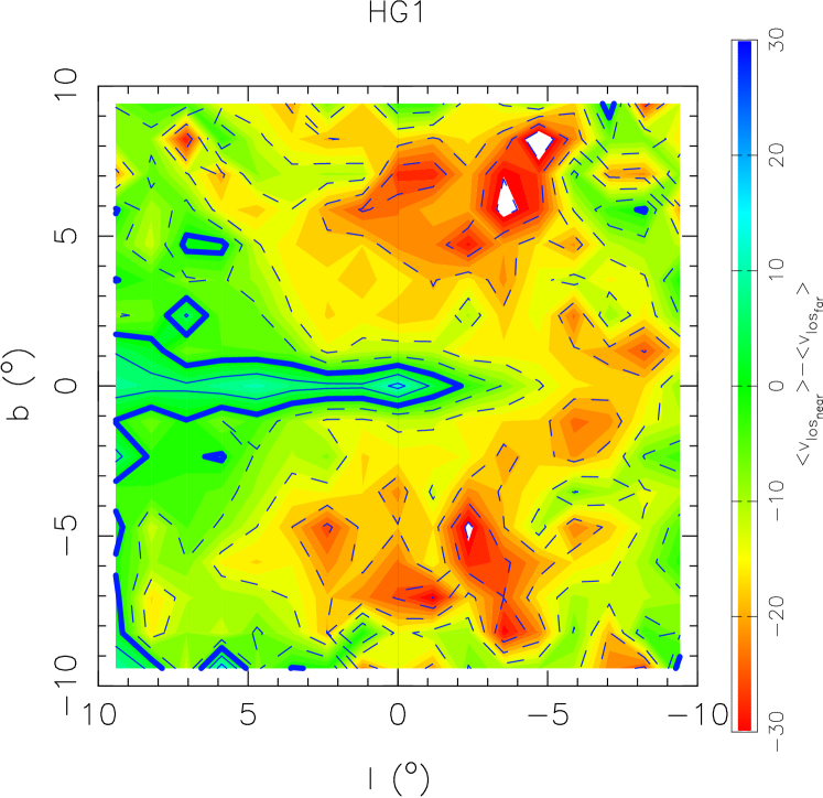
Figure 15: Model HG1 with gas and star formation. Top panel: Three orthogonal projections of the model as seen from outside the system with the bar rotated into the $x$-axis. Middle panel: Density in the $l=0\degr$ plane. The region $|b|<1\degr$ is dominated by the disc. Bottom panel: Difference between near and far side mean line-of-sight velocity.

We now consider simulation HG1 in which a disc forms from a cooling gas corona embedded in a live dark matter halo. This simulation has not been published before but uses the approach described in Roškar et al. (2008) with higher resolution. By the end of the simulation, at 10 Gyr, the disc consists of $\sim 1.1\times 10^{7}$ particles. A bar obviously forms with an X-shape. The top panel of Fig. 15 shows the density distribution; the bar has a radius of about 3 kpc. A boxy bulge is also visible in the edge-on projection. For the purposes of this paper we do not scale this bar to the Milky Way, merely using it to demonstrate that the kinematic signature of an X-shaped bulge is also present in this more realistic simulation, rather than being a feature of bars forming within frozen dark matter haloes. The middle panel of Fig. 15 demonstrates that the bulge has an X-shape when viewed in the $l=0$ plane. This model, unlike the other models, also has a conspicuous disc at $|b|<1\degr$, outside the region where the Milky Way’s X-shape is found. Finally, the bottom panel of Fig. 15 presents a map of the difference between the near and far side mean line-of-sight velocity. At $|b|<1\degr$ the kinematics are strongly contaminated by the inner disc, so we ignore this region in our analysis; We find that the signature of the X-shape is still present as a minimum in the velocity difference at $|b|\simeq 7\degr$. Thus we are confident that a minimum in near-far side difference in mean line-of-sight velocities at $l=0\degr$ constitutes a signature of an X-shaped bulge.

6 Measuring the distance to the Galactic Centre using the X-shape

McWilliam & Zoccali (2010) present a distribution of RC stars (their fig. 8) and measure the distance to the centre of the Galaxy using the X-shape in the RC stars traced in the $l=0\degr$ plane. We explore the potential for using the X-shape for determining the distance to the Galactic Centre by measuring the ridge of highest density along the line-of-sight on the near and far sides of the bulge, excluding any central peaks. Latitudes $|b|<4\degr$ fail to find a peak off the centre, therefore we include only the lines-of-sight at $|b|\geq 4\degr$ sampling every 0.25° up to $|b|$ = 8°, for a total of 17 measurements per arm. Each sample covers $0.5\degr\times 0.5\degr$. Then we fit a line to each of the four arms of the X-shape. Fig. 16 shows the measured positions of the arms in our models as traced by the peak density, while the dotted lines show the linear fits to each arm. By using the arms alone, it is possible to measure the distance to the galactic centre to within 2.5%, although the lower two arms of B3 give a result accurate to only 4%. The increased error in B3 arises because the fit to the two arms closer to the observer have a much shallower slope, so that the uncertainty in the slope translates into a relatively large variation in the intersection with the linear fit to the far side arm. The solid lines in Fig. 16 show the linear fits for arms at opposite corners of the X-shape (e.g. top-left and bottom-right). The fit to the full X-shape almost exactly finds the centre, to within better than a tenth of a per cent for both models.

Either method for measuring the distance to the galactic centre works well, although the full shape seems to constrain the system better. We note that the asymmetry across the mid-plane of model R1 does not translate into a problem for the galactic centre distance determination. In the Milky Way observations linking positive and negative latitudes may be subject to greater uncertainty than those at only positive or only negative latitudes.

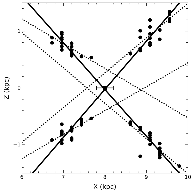
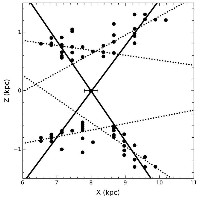
Figure 16: Positions of the density peaks along the line-of-sight at $l=0\degr$, $4\degr<|b|\leq 8\degr$ for R1 (top) and B3 (bottom). The measurements are every 0.25 deg and each point covers an area of 0.25 deg². The dotted lines represent linear fits to each arm of the X-shape. The solid lines show linear fits joining arms diagonal from each other. The square denotes the position of the centre, while the error bar indicates an error of 2.5%.

This implies that given a good enough distance determination of the arms of the X-shape it should be possible to measure the position of the Galactic Centre to within a few hundred parsec. In order to understand how random errors would affect the distance determination, we mapped each arm with five points ($b$ $=\pm 4\degr,5\degr,6\degr,7\degr,8$°), and fitted a linear relation for the X-shape. We then measure the galactic centre as before using the method of fitting the diagonal arms, determining the accuracy of the distance measurement after adding a random error uniformly distributed between $-10$ and $10$ per cent or $-20$ and $20$ per cent to each measurement of a peak along an arm. We repeat this procedure one million times. We find that linear fits are able to measure the distance to within 5% or better at least 96.5% per cent of the time, as seen in Table 2. The 20% error limit, for Gaia, requires an accuracy of 25 $\mu as$ at a distance of 8 kpc for an individual star. This level of accuracy is obtainable for stars with magnitudes of $G<16$ (Lindegren et al., 2012). From Robin et al. (2005) and Reylé et al. (2008), using three different extinction models (Schlegel et al., 1998; Schultheis et al., 1999; Marshall et al., 2006) , it is clear that RC stars at $|b|>4\degr$ will be reached by Gaia at G $<$ 16, even with extinction, which is anyway low at these latitudes. Since the method relies on locating the density peak, which relies on distance determinations of many stars, the uncertainty on individual peaks with Gaia should be much less than $20\%$. Thus this purely geometric method, which focuses on a region of the Milky Way which is much less extincted, promises to significantly improve our measurement of the distance to the Galactic Centre.

Table 2: Error distribution in the measurement of distance using the X-shape with lines joining diagonal arms. Each column contains the fraction of distance measurements that are within the given error, out of the total one million Monte Carlo experiments.

Model	Assumed	$\leq$2.5%	$\leq 5\%$	$\leq 7.5\%$
	error
R1	10%	0.904	0.999	0.999
R1	20%	0.825	0.965	0.996
B3	10%	0.939	0.999	0.999
B3	20%	0.846	0.970	0.996

7 Discussion and conclusions

Our analysis shows that the primary kinematic imprint of an X-shape is in the difference between the mean line-of-sight velocities, $V_{los}$, of the near and far sides of the bulge. In the $l=0\degr$ plane, the presence of an X-shape leads to a minimum in this difference at $|b|\sim 4\degr$. At this latitude the arms of the X-shape can be hard to distinguish but the difference is unmistakably due to the X-shape. It bears repeating that the kinematic evidence of the X-shape is not just a difference between near and far side mean $V_{los}$, but rather a minimum in this difference. Differences between mean Galactocentric azimuthal velocities, while non-zero, do not show a qualitatively different behaviour between models with and without an X-shape. The vertical velocities are even more unable to distinguish whether an X-shape is present or not. The velocity dispersions in all these quantities also show no qualitative difference between systems with and without an X-shape. Therefore we recommend better measurements of RC velocities across $3\degr\la|b|\la 7\degr$ at $l=0\degr$.

Our comparison with simulations also highlights the relatively poor discriminating power of the available kinematics in the bulge region. Both model R1, with only a bar induced B/P-shaped bulge, and model B3, which included a classical bulge from the start, are able to fit most of the observational kinematic data to a surprising degree. Indeed the details of the X-shape provide more of a distinction than do the kinematics. Unfortunately therefore, while it is clear that the bulge of the Milky Way has been sculpted by the bar, the current kinematic data cast no light on whether the bulge is a pre-existing structure (a classical bulge) or one forged by secular evolution (a pseudo bulge). We emphasize that this is a result of the still sparse sampling of velocities with relatively large uncertainties. In particular we note that the kinematic signature of the X-shape in model B3 is carried largely by the disc, not by the classical bulge. Moreover the classical bulge itself has a boxy shape, not an X-shape. These properties may aid future studies to determine the contribution of a classical bulge to the Milky Way’s bulge.

The available kinematic data however provide strong constraints on the orientation of the bar relative to the line-of-sight to the Galactic Centre. For both models (R1 and B3), the best-fitting bar angle, compared with the BRAVA data, is consistently 15°.. This value is between the 13° value from Robin et al. (2012) and the 20° value from Li & Shen (2012). It is unclear whether this is driven by the selection functions, or is a real result based on the best fit to BRAVA data. Our models show that the relative distributions of near versus far line-of-sight velocities in the region of the X-shape can provide stronger constraints on the bar angle.

Finally we showed that it should be possible to measure the distance to the Galactic Centre to quite high accuracy using the X-shape. By tracing the location of the density peaks in the arms along the line-of-sight, and fitting lines to them, we were able to measure the distance to the Galactic Centre in the models to accuracy of at least 5 per cent 96% of the time. This requires measurements of the positions of the density peaks along each arm with uncertainties of $20\%$. Measurements with Gaia can constrain the distances to the arms with comparable or better accuracy. The major advantages of this method are that it is purely geometric, works even if the X-shape is not perfectly symmetric across the mid-plane, and looks at regions of the bulge which are away from the heavily-extincted main plane of the disc. We anticipate that in the era of Gaia we shall be able to make high accuracy measurements of the distance to the Galactic Centre using this method.

Appendix A Analysis of six unscaled models

We concentrate here on the analysis of all six models, with a few simplifications. The distance of the observer to the centre is set to 2 bar lengths, and the models are completely unscaled. The comparisons of the models will be qualitative, instead of quantitative, as in the main part of the paper. All models have been rotated so that the bar angle is $15\degr$.

Of the models in Fig. 17, R1 and B3 exhibit strong B/P shapes, B2 and R5 have weak B/P shapes, while R6 does not have an X-shape at all. R2 is a special case where there is an X-shape, but it requires a much larger observer distance to see it at $|b|<8\degr$.

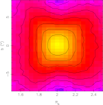
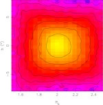
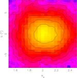
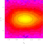
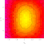
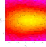
Figure 17: Density of models R1 (top-left), B3 (top-right), B2 (middle-left), R5 (middle-right), R2 (bottom-left) and R6 (bottom-right) in the $l=0\degr$ plane. The plot shows the density as a function of latitude and distance, mimicking the projection in Fig. 4 of Saito et al. (2011). The models are ordered by their overall boxiness, with the last two exhibiting no signs of a visible X-shape.

A.1 Velocities

The presence of the X-shape is evident in the difference between mean $V_{los}$ (Figs 18 and 19). The differences in galactocentric $V_{\phi}$ and $\sigma_{\phi}$ (Figs 20 and 21 show no evidence of the imprint of an X-shape. Both vertical velocity (Fig. 22) and vertical velocity dispersion (Fig. 23) show no signs of coherent differences between means on the near and far sides.

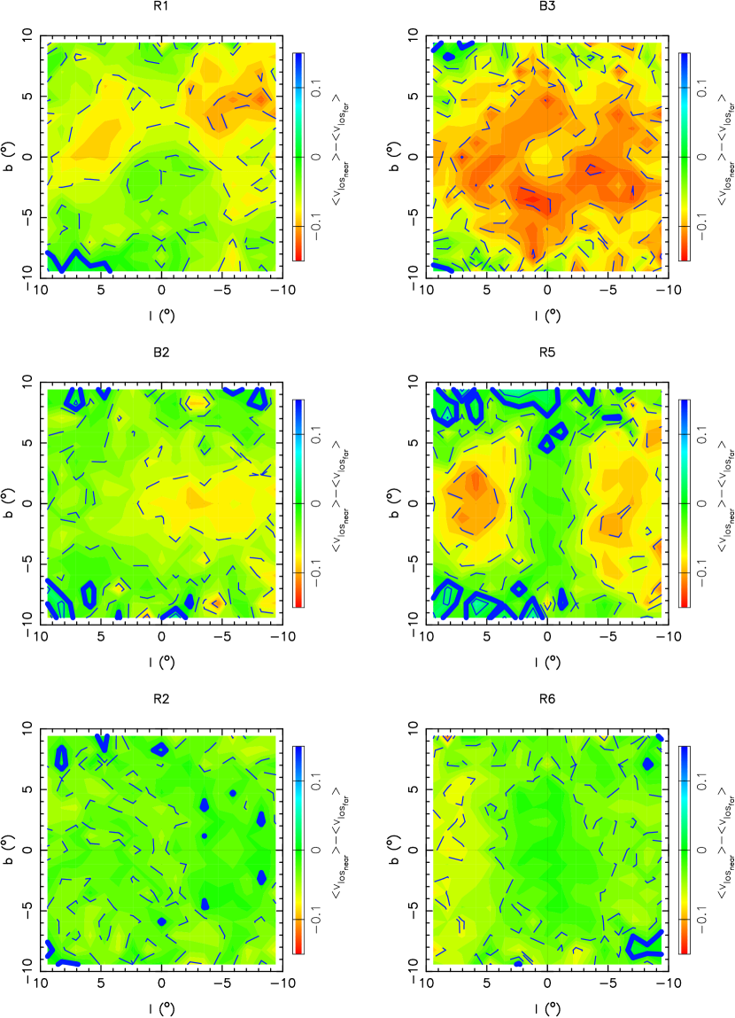
Figure 18: The difference in mean line-of-sight velocity ($V_{los}$) between the near and far sides of the bulge, for a bar angle of 15°, for each simulation. The dashed lines show negative contours while the bold contour shows 0 km s^-1.

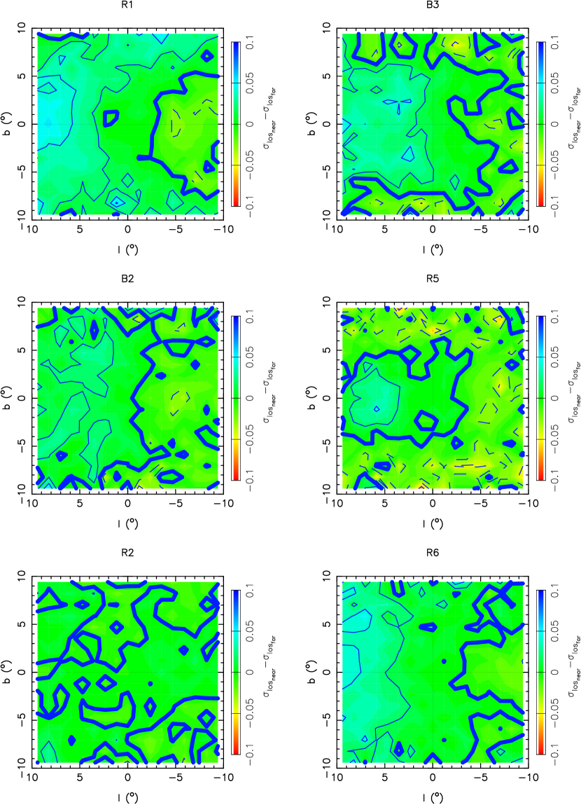
Figure 19: The difference in line-of-sight velocity dispersion ($\sigma_{los}$) between the near and far sides of the bulge, for a bar angle of 15°, for each simulation. The dashed lines show negative contours while the bold contour shows 0 km s^-1.

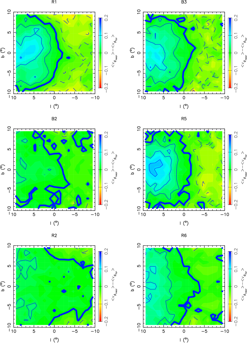
Figure 20: Same as Fig. 18, for galactocentric azimuthal velocity (V_ϕ).

Figure 21: Same as Fig. 19, for galactocentric azimuthal velocity dispersion ($\sigma_{\phi}$).

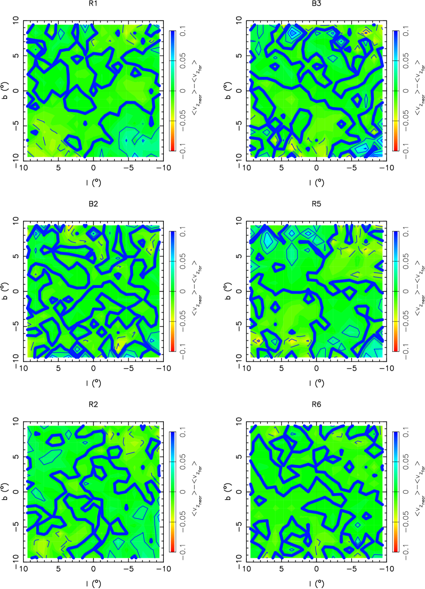
Figure 22: Same as Fig. 18, for vertical velocity (V_z).

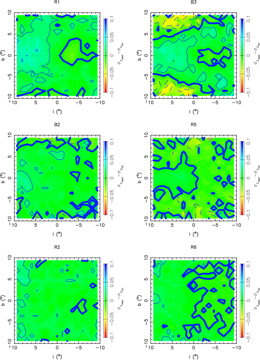
Figure 23: Same as Fig. 19, for vertical velocity dispersion ($\sigma_{z}$).

A.2 The effect of bar angle on velocities

An asymmetric bulge should show velocity distributions which change as the viewing angle changes. In Fig. 24, 25 and 26 we show the distributions of near and far side velocities for bar angles $15\degr$, $25\degr$ and $35\degr$ at $(l,b)=(0\degr,-6\degr)$. For the X-shaped models, R1 and B3, the $V_{los}$ distributions are different and change considerably with bar angle; the distributions are less separated and show less relative change in the rest of the models. This latitude therefore is a sensitive probe of the bar angle in $V_{los}$. Azimuthal (Fig. 25) and vertical velocities (Fig. 26) are mostly unaffected by the change in bar angle. The absence of a near/far side asymmetry shows little dependence on bar angle.

Angle: 15∘	25∘	35∘
R1
B3
B2
R5
R2
R6

Figure 24: Distribution of line-of-sight velocities V_los, at ($l,b$) = (0°,$-$6°), for varying bar angles in the six simulations. The solid line, in each panel, is the far side of the model, while the dashed line is the near side of the model. The models that exhibit an X-shape show near/far asymmetry, at all bar angles. Those without an X-shape do not exhibit comparable asymmetry.

Angle: 15∘	25∘	35∘
R1
B3
B2
R5
R2
R6

Figure 25: Same as Fig. 24 for galactocentric azimuthal velocities, V_ϕ. None of the models exhibit substantial near/far asymmetry.

Angle: 15∘	25∘	35∘
R1
B3
B2
R5
R2
R6

Figure 26: Same as Fig. 24 for vertical velocities, V_z. None of the models exhibit substantial near/far asymmetry.

A.3 Conclusions from all models

Models with X-shapes have a distinct signature in the difference between near and far sides mean line-of-sight velocity only. This signature is not present in models without X-shapes. Additionally, the bar angle has an effect on these asymmetries.

References

- Athanassoula (2003) Athanassoula E., 2003, MNRAS, 341, 1179
- Athanassoula (2005) Athanassoula E., 2005, MNRAS, 358, 1477
- Baugh et al. (1996) Baugh C. M., Cole S., Frenk C. S., 1996, MNRAS, 283, 1361
- Bettoni & Galletta (1994) Bettoni D., Galletta G., 1994, A&A, 281, 1
- Binney et al. (1997) Binney J., Gerhard O., Spergel D., 1997, MNRAS, 288, 365
- Bissantz & Gerhard (2002) Bissantz N., Gerhard O., 2002, MNRAS, 330, 591
- Burbidge & Burbidge (1959) Burbidge E. M., Burbidge G. R., 1959, ApJ, 130, 20
- Bureau & Freeman (1999) Bureau M., Freeman K. C., 1999, AJ, 118, 126
- Chung & Bureau (2004) Chung A., Bureau M., 2004, AJ, 127, 3192
- Clarkson et al. (2008) Clarkson W. et al., 2008, ApJ, 684, 1110
- Clarkson et al. (2011) Clarkson W. I. et al., 2011, ApJ, 735, 37
- Combes et al. (1990) Combes F., Debbasch F., Friedli D., Pfenniger D., 1990, A&A, 233, 82
- Combes & Sanders (1981) Combes F., Sanders R. H., 1981, A&A, 96, 164
- Courteau et al. (1996) Courteau S., de Jong R. S., Broeils A. H., 1996, ApJ, 457, L73
- De Propris et al. (2011) De Propris R. et al., 2011, ApJ, 732, L36
- Debattista et al. (2004) Debattista V. P., Carollo C. M., Mayer L., Moore B., 2004, ApJ, 604, L93
- Debattista et al. (2005) Debattista V. P., Carollo C. M., Mayer L., Moore B., 2005, ApJ, 628, 678
- Debattista et al. (2006) Debattista V. P., Mayer L., Carollo C. M., Moore B., Wadsley J., Quinn T., 2006, ApJ, 645, 209
- Driver et al. (2011) Driver S. P. et al., 2011, MNRAS, 413, 971
- Drory & Fisher (2007) Drory N., Fisher D. B., 2007, ApJ, 664, 640
- Dwek et al. (1995) Dwek E. et al., 1995, ApJ, 445, 716
- Eggen et al. (1962) Eggen O. J., Lynden-Bell D., Sandage A. R., 1962, ApJ, 136, 748
- Erwin et al. (2003) Erwin P., Beltrán J. C. V., Graham A. W., Beckman J. E., 2003, ApJ, 597, 929
- Erwin & Debattista (2013) Erwin P., Debattista V. P., 2013, MNRAS, 431, 3060
- Fukugita et al. (1998) Fukugita M., Hogan C. J., Peebles P. J. E., 1998, ApJ, 503, 518
- Fux (1999) Fux R., 1999, A&A, 345, 787
- Hopkins et al. (2010) Hopkins P. F. et al., 2010, ApJ, 715, 202
- Howard et al. (2009) Howard C. D. et al., 2009, ApJ, 702, L153
- Kauffmann et al. (1993) Kauffmann G., White S. D. M., Guiderdoni B., 1993, MNRAS, 264, 201
- Kormendy & Kennicutt (2004) Kormendy J., Kennicutt Jr. R. C., 2004, ARA&A, 42, 603
- Kuijken & Merrifield (1995) Kuijken K., Merrifield M. R., 1995, ApJ, 443, L13
- Kuijken & Rich (2002) Kuijken K., Rich R. M., 2002, AJ, 124, 2054
- Kunder et al. (2012) Kunder A. et al., 2012, AJ, 143, 57
- Laurikainen et al. (2011) Laurikainen E., Salo H., Buta R., Knapen J. H., 2011, MNRAS, 418, 1452
- Li & Shen (2012) Li Z.-Y., Shen J., 2012, ApJ, 757, L7
- Lindegren et al. (2012) Lindegren L., Lammers U., Hobbs D., O’Mullane W., Bastian U., Hernández J., 2012, A&A, 538, A78
- López-Corredoira et al. (2005) López-Corredoira M., Cabrera-Lavers A., Gerhard O. E., 2005, A&A, 439, 107
- Lütticke et al. (2000) Lütticke R., Dettmar R.-J., Pohlen M., 2000, A&AS, 145, 405
- Marshall et al. (2006) Marshall D. J., Robin A. C., Reylé C., Schultheis M., Picaud S., 2006, A&A, 453, 635
- McWilliam (1997) McWilliam A., 1997, ARA&A, 35, 503