Some Properties of Bilayer Graphene Nanoribbons

Abstract

In this work the tight binding model calculations are carried out for AA-Bilayer Graphene nanoribbons as an example of bilayer systems. The effects of edges, NNN hopping, and impurities of a single layer are introduced numerically as a change in the elements of the relevant block diagonal matrix appearing in the direct diagonalization method. The direct interlayer hopping between the top and the bottom single layers is constructed in the generalized direct diagonalization method by the off-diagonal block matrices in which the strength of the interlayer hopping is included.

I Introduction

In the previous work Ahmed (2011a, b), we have studied the effects of lattice structures (including both the honeycomb and square lattices), the interaction range (NN and NNN), and the presence of impurities on the dispersion relations of the 2D materials. This was carried out both for graphene nanoribbons and magnetic stripes in order to compare and contrast their behavior. The intrinsic physical properties of 2D materials may not, in general, be easily tunable and therefore they cannot necessarily meet many technological applications design requirements. However, it has been proposed in the literature that a system of two graphene layers stacked on top of each other might give rise to the possibility of controlling their physical properties by introducing asymmetry between the layers. This could be done in various ways like varying the external electric or magnetic field, rotation between the two layers, and introducing impurities in one layer Castro et al. (2010); Xu et al. (2009); Kalon et al. (2011); Trambly de Laissardière et al. (2010); Ohta et al. (2006). This opens the possibility of technological applications using bilayer graphene D.S.L. Abergel and Chakraborty (2010).

In this work, we will extend our formalism for single-layer graphene as developed in Ahmed (2011b, a) to examine the effect of forming a system of two layers stacked on top of each other. We then derive the dispersion relations and study the localized edge modes. Specifically, the system that will be used for our study consists of two graphene layers stacked directly on top of each other to form what is called AA-stacking bilayer graphene (BLG) nanoribbons. This system is interesting both experimentally and theoretically Liu et al. (2009); Fang-Ping et al. (2011); Chang et al. (2010); de Andres et al. (2008).

The tight binding Hamiltonian D.S.L. Abergel and Chakraborty (2010); Castro Neto et al. (2009) will be used as before to describe the NN and NNN hopping in each graphene single layer (GSL), while additional tight binding terms are introduced to describe the direct hopping between the two layers D.S.L. Abergel and Chakraborty (2010); Castro Neto et al. (2009). As well as the main applications to graphene bilayer nanoribbons, the results should also be capable of extension to similar magnetic stripes in bilayer configurations which could be fabricated as ”nanodot” arrays Jiang (1996); Belkin et al. (2008); Beutier et al. (2005); Carapella et al. (2009).

II Theoretical model

The system initially under study consists of two graphene layers stacked directly on top of each other, i.e., AA-stacking bilayer graphene (BLG) nanoribbons in the $xy$-plane, where we use the indices “t” and “b” to label the top and bottom layer, respectively. The crystallographic description of each graphene layer with its honeycomb lattice is given in D.S.L. Abergel and Chakraborty (2010); Castro Neto et al. (2009). The bilayer nanoribbon is of finite width in the $y$ direction with $N$ atomic rows (labeled as $n=1,\cdots,N$) and it is infinite in the $x$ direction (see Figure 1).

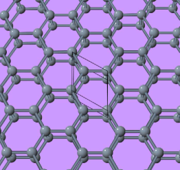
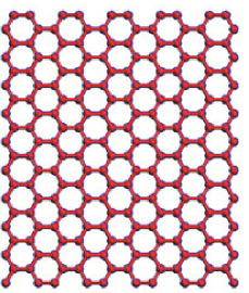
Figure 1: Direct on-top AA-stacking bilayer graphene (BLG). Left: the 2D unit cell is shown $a=b=0.267nm$, $\gamma=120^{\circ}$. Right: AA-stacking BLG nanoribbons. Figures taken from de Andres et al. (2008); Chang et al. (2010).

The total Hamiltonian of the system is given as follows:

$$\hat{H}=\hat{H}_{t}+\hat{H}_{b}+\hat{H}_{i},$$ (1)

where $\hat{H}_{t}$ ($\hat{H}_{b}$) is the Hamiltonian of the top (bottom) single layer of graphene (SLG) which describes the in-plane hopping of non-interacting $\pi$-electrons on the top (bottom) layer and it is given by

$$\hat{H}_{t} = -\sum_{\langle ij,t\rangle}t_{{0}_{ij},t}(\textbf{a}^{\dagger}_{i,t}\textbf{b}_{j,t}+\textbf{h.c})+t_{{1}_{ij},t}(\textbf{a}^{\dagger}_{i,t}\textbf{a}_{j,t}+\textbf{b}^{\dagger}_{i,t}\textbf{b}_{j,t}+\textbf{h.c}),$$

$$\hat{H}_{b} = -\sum_{\langle ij,b\rangle}t_{{0}_{ij},b}(\textbf{a}^{\dagger}_{i,b}\textbf{b}_{j,b}+\textbf{h.c})+t_{{1}_{ij},b}(\textbf{a}^{\dagger}_{i,b}\textbf{a}_{j,b}+\textbf{b}^{\dagger}_{i,b}\textbf{b}_{j,b}+\textbf{h.c}).$$ (2)

The notation is defined as follows the first term in each layer $t_{0_{ij}}(\approx 2.8\textrm{eV})$ is the NN hopping energy, and here in graphene it is the hopping between different sublattices $A$ and $B$. Also $t_{1_{ij}}(\approx 0.1\textrm{eV})$ is the NNN hopping energy in each layer which here in graphene is the hopping in the same sublattice Castro Neto et al. (2009); Deacon et al. (2007); Reich et al. (2002). The summations in each layer over $i$ and $j$ run over all the sites where $i$ and $j$ belong to different sublattices for the NN hopping term, and they belong to the same sublattice for the NNN hopping energy. The labeling schemes for the various hopping terms (at an edge or in the interior) are the same as in the previous work for the single-layer case.

The third term in the total Hamiltonian $\hat{H}_{i}$ represents the Hamiltonian of the direct inter-layer hopping between the top and the bottom single layers where the sublattice $A_{t}$ ($B_{t}$) of the top layer is directly above the sublattice $A_{t}$ ($B_{t}$) of the bottom layer. It is given by

$$\hat{H}_{i}=-\sum_{\langle i\rangle}\gamma_{0}(\textbf{a}^{\dagger}_{i,b}\textbf{a}_{i,t}+\textbf{b}^{\dagger}_{j,b}\textbf{b}_{j,t}+\textbf{h.c}),$$ (3)

where $\gamma_{0}$ the inter-layer NN coupling energy.

Since the nanoribbon extends to $\pm\infty$ in the $x$ direction, we may introduce a 1D Fourier transform to wavevector $q_{x}$ along the $x$ direction for the fermions operators $a^{{\dagger}}_{i}$ ($a_{i}$) and $b^{{\dagger}}_{j}$ ($b_{j}$) in each layer as follows:

$$b_{j}(x) =\frac{1}{\sqrt{N_{0}}}\sum_{n}b_{n}(q_{x})e^{-i\mathbf{q}_{x}\cdot\mathbf{r}_{j}},\hskip 20.0ptb_{j}^{\dagger}(x)=\frac{1}{\sqrt{N_{0}}}\sum_{n}b^{\dagger}_{n}(q_{x})e^{i\mathbf{q}_{x}\cdot\mathbf{r}_{j}},$$

$$a_{i}(x) =\frac{1}{\sqrt{N_{0}}}\sum_{n}a_{n}(q_{x})e^{-i\mathbf{q}_{x}\cdot\mathbf{r}_{i}},\hskip 20.0pta_{i}^{\dagger}(x)=\frac{1}{\sqrt{N_{0}}}\sum_{n}a^{\dagger}_{n}(q_{x})e^{i\mathbf{q}_{x}\cdot\mathbf{r}_{i}}.$$ (4)

Here, $N_{0}$ is the (macroscopically large) number of carbon sites in any row, $\mathbf{q_{x}}$ is a wavevector in the first Brillouin zone of the reciprocal lattice and both $\mathbf{r}_{i}$ and $\mathbf{r}_{j}$ denote the position vectors of any carbon sites $i$ and $j$. The new fermion operators obey the following anticommutation relations in each layer:

$$\left[a_{n}(q_{x}),a^{\dagger}_{n}(q^{\prime}_{x})\right]=\delta_{q_{x}q^{\prime}_{x}},\hskip 30.0pt\left[b_{n}(q_{x}),b^{\dagger}_{n}(q^{\prime}_{x})\right]=\delta_{q_{x}q^{\prime}_{x}},$$ (5)

while the top layer operators anticommute with the bottom layer operators. Also, we define the hopping sums

$$\tau(q_{x}) = \sum_{\nu}t_{{0}_{ij}}e^{-i\mathbf{q}_{x}\cdot(\mathbf{r}_{i}-\mathbf{r}_{j})},$$

$$\tau^{\prime}(q_{x}) = \sum_{\nu^{\prime}}t_{{1}_{ij}}e^{-i\mathbf{q}_{x}\cdot(\mathbf{r}_{i}-\mathbf{r}_{j})}.$$ (6)

The sum for the hopping terms $t_{{0/1}_{ij}}$ is taken to be over all $\nu$ NNs and over all $\nu^{\prime}$ NNNs in the lattice and this depends on the edge configuration as zigzag or armchair for the stripe (see Ahmed (2011a)). For the inter-layer coupling the in-plane wavevector $\mathbf{q}_{x}$ is perpendicular to the inter-plane vector and so the hopping sum is only $\gamma_{0}$ representing the corresponding NN coupling energy.

For the armchair configuration, the hopping sum for NNs gives the following factors $\tau_{nn^{\prime}}(q_{x})$ for each (top or bottom) layer:

$$\tau_{nn^{\prime}}(q_{x})=t\left[\exp(iq_{x}a)\delta_{n^{\prime},n}+\exp\left(i\frac{1}{2}q_{x}a\right)\delta_{n^{\prime},n\pm 1}\right]$$ (7)

and for the zigzag configuration, it gives:

$$\tau_{nn^{\prime}}(q_{x})=t\left[2\cos\left(\frac{\sqrt{3}}{2}q_{x}a\right)\delta_{n^{\prime},n\pm 1}+\delta_{n^{\prime},n\mp 1}\right].$$ (8)

Explicitly the hopping sum for NNNs gives the following factors $\tau^{\prime}_{nn^{\prime}}(q_{x})$ for each layer

$$\tau_{nn^{\prime}}(q_{x})=t^{\prime}\left[\delta_{n^{\prime},n\pm 2}+2\cos(q_{x}a3/2)\delta_{n^{\prime},n\pm 1}\right]$$ (9)

for the armchair configuration, and

$$\tau_{nn^{\prime}}(q_{x})=2t^{\prime}\left[\cos(\sqrt{3}q_{x}a)\delta_{n^{\prime},n}+\cos(\sqrt{3}q_{x}a/2)\delta_{n^{\prime},n\pm 2}\right]$$ (10)

for the zigzag configuration case, where the $\pm$ sign, in all the above factors, depends on the sublattice since the atom lines alternate between the A and B sublattices.

Substituting Equations (4) and (6) in Equation (1), and rewriting the summation over NN and NNN sites, we get the following form of the total Hamiltonian operator $\hat{H}$:

$$\hat{H} = -\sum_{nn^{\prime},t}\tau^{\prime}(q_{x})_{t}\left(a^{\dagger}_{n,t}a_{n^{\prime},t}+b^{\dagger}_{n,t}b_{n^{\prime},t}\right)+\tau(q_{x})_{t}a_{n,t}b^{\dagger}_{n^{\prime},t}+\tau(-q_{x})_{t}a^{\dagger}_{n,t}b_{n^{\prime},t}$$ (11)

$$-\sum_{nn^{\prime},b}\tau^{\prime}(q_{x})_{b}\left(a^{\dagger}_{n,b}a_{n^{\prime},b}+b^{\dagger}_{n,b}b_{n^{\prime},b}\right)+\tau(q_{x})_{b}a_{n,b}b^{\dagger}_{n^{\prime},b}+\tau(-q_{x})_{b}a^{\dagger}_{n,b}b_{n^{\prime},b}$$

$$-\sum_{n}\gamma_{0}(a^{\dagger}_{n,b}a_{n,t}+b^{\dagger}_{n,b}b_{n,t}+H.c.),$$

where the first two lines account for the NN and NNN intra-layer hopping in the t and b layers, respectively, and the third line represent inter-layer hopping.

In order to diagonalize $\hat{H}$ and obtain the dispersion relations for AA-stacking bilayer graphene (BLG) nanoribbons, we may consider the modified time evolution of the creation and the annihilation operators $a^{{\dagger}}_{i}$ ($a_{i}$) and $b^{{\dagger}}_{j}$ ($b_{j}$), as calculated in the Heisenberg picture in quantum mechanics. In this case, the equations of motion (using the units with $\hbar=1$) for the annihilation operators $a_{i}$($b_{j}$) are as follows B s (2007); Liboff (1987); Kantorovich (2004); R ssler (2009); Henrik Bruus (2004):

$$\frac{da_{n,t}}{dt} = i[H,a_{n,t}]=i[H_{t}+H_{b}+H_{i},a_{n,t}]$$ (12)

$$= i\sum_{nn^{\prime}}-\tau^{\prime}(q_{x})a_{n^{\prime},t}-\tau(-q_{x})b_{n^{\prime},t}-\gamma_{0}a_{n,b}$$

and

$$\frac{db_{n,t}}{dt} = i[H,b_{n,t}]=i[H_{t}+H_{b}+H_{i},b_{n,t}]$$ (13)

$$= i\sum_{nn^{\prime}}-\tau^{\prime}(q_{x})b_{n^{\prime},t}-\tau(q_{x})a_{n^{\prime},t}-\gamma_{0}b_{n,b}$$

for the operators of the top layer. Similarly for the bottom layer we have

$$\frac{da_{n,b}}{dt} = i\sum_{nn^{\prime}}-\tau^{\prime}(q_{x})a_{n^{\prime},b}-\tau(-q_{x})b_{n^{\prime},b}-\gamma_{0}a_{n,t}$$

$$\frac{db_{n,b}}{dt} = i\sum_{nn^{\prime}}-\tau^{\prime}(q_{x})b_{n^{\prime},b}-\tau(q_{x})a_{n^{\prime},b}-\gamma_{0}b_{n,t}$$ (14)

where Equation (5) was used.

The electronic dispersion relations of the double-layer graphene (i.e., energy or frequency versus wavevector) can now be obtained by solving the above operator equations of motion. Assuming, as before, that the coupled electronic modes behave like $\exp[-i\omega(q_{x})t]$, on substituting this time dependent form into Equations 12-14, we get the following set of coupled equations:

$$\omega(q_{x})a_{n,t} = \sum_{n^{\prime}}\tau^{\prime}_{nn^{\prime}}(q_{x})a_{n^{\prime},t}+\tau_{nn^{\prime}}(-q_{x})b_{n^{\prime},t}+\gamma_{0}a_{n,b}$$

$$\omega(q_{x})b_{n,t} = \sum_{n^{\prime}}\tau_{nn^{\prime}}(q_{x})a_{n^{\prime},t}+\tau^{\prime}_{nn^{\prime}}(q_{x})b_{n^{\prime},t}+\gamma_{0}b_{n,b}$$

$$\omega(q_{x})a_{n,b} = \sum_{n^{\prime}}\tau^{\prime}_{nn^{\prime}}(q_{x})a_{n^{\prime},b}+\tau_{nn^{\prime}}(-q_{x})b_{n^{\prime},b}+\gamma_{0}a_{n,t}$$

$$\omega(q_{x})b_{n,b} = \sum_{n^{\prime}}\tau_{nn^{\prime}}(q_{x})a_{n^{\prime},b}+\tau^{\prime}_{nn^{\prime}}(q_{x})b_{n^{\prime},b}+\gamma_{0}b_{n,t}$$ (15)

The above equations can be written in matrix form as follows:

$$\omega(q_{x})\left[\begin{array}[]{c}a_{n,t}\\ b_{n,t}\\ a_{n,b}\\ b_{n,b}\\ \end{array}\right] = \left[\begin{array}[]{cccc}T_{t}^{\prime}(q_{x})&T_{t}(q_{x})&U&0\\ T_{t}^{*}(q_{x})&T_{t}^{\prime}(q_{x})&0&U\\ U&0&T_{b}^{\prime}(q_{x})&T_{b}(q_{x})\\ 0&U&T_{b}^{*}(q_{x})&T_{b}^{\prime}(q_{x})\\ \end{array}\right]\left[\begin{array}[]{c}a_{n,t}\\ b_{n,t}\\ a_{n,b}\\ b_{n,b}\\ \end{array}\right]\,$$ (28)

where the solution of this matrix equation is given by the determinantal condition

$$\det\left[\begin{array}[]{cccc}-R(q_{x})_{t}&T_{t}(q_{x})&U&0\\ T_{t}^{*}(q_{x})&-R(q_{x})_{t}&0&U\\ U&0&-R(q_{x})_{b}&T_{b}(q_{x})\\ 0&U&T_{b}^{*}(q_{x})&-R(q_{x})_{b}\\ \end{array}\right]=0$$ (33)

where we denote $R(q_{x})_{t}=\omega(q_{x})I_{N}-T_{t}^{\prime}(q_{x})$ , and for each layer $T(q_{x})$ and $T^{\prime}(q_{x})$ are the NN and NNN interaction matrices respectively, which depend on the orientation of the ribbon, and $\omega(q_{x})$ are the energies of the modes. The matrix $T(q_{x})$ is given by

$$\left(\begin{array}[]{ccccc}\alpha&\beta&0&0&\cdots\\ \beta&\alpha&\gamma&0&\cdots\\ 0&\gamma&\alpha&\beta&\cdots\\ 0&0&\beta&\alpha&\cdots\\ \vdots&\vdots&\vdots&\vdots&\ddots\\ \end{array}\right).$$ (34)

whereas the NNN matrix $T^{\prime}(q_{x})$ for zigzag ribbons is given by

$$\left(\begin{array}[]{cccccc}\epsilon&0&\zeta&0&0&\cdots\\ 0&\epsilon&0&\zeta&0&\cdots\\ \zeta&0&\epsilon&0&\zeta&\cdots\\ 0&\zeta&0&\epsilon&0&\cdots\\ 0&0&\zeta&0&\epsilon&\cdots\\ \vdots&\vdots&\vdots&\vdots&\vdots&\ddots\\ \end{array}\right)$$ (35)

and the matrix $T^{\prime}(q_{x})$ for armchair ribbons is given by

$$\left(\begin{array}[]{cccccc}0&\eta&\theta&0&0&\cdots\\ \eta&0&\eta&\theta&0&\cdots\\ \theta&\eta&0&\eta&\theta&\cdots\\ 0&\theta&\eta&0&\eta&\cdots\\ 0&0&\theta&\eta&0&\cdots\\ \vdots&\vdots&\vdots&\vdots&\vdots&\ddots\\ \end{array}\right)$$ (36)

Finally, $U$ is the inter-layer hopping coupling matrix and it is given by

$$\left(\begin{array}[]{cccccc}\gamma_{0}&0&0&0&0&\cdots\\ 0&\gamma_{0}&0&0&0&\cdots\\ 0&0&\gamma_{0}&0&0&\cdots\\ 0&0&0&\gamma_{0}&0&\cdots\\ 0&0&0&0&\gamma_{0}&\cdots\\ \vdots&\vdots&\vdots&\vdots&\vdots&\ddots\\ \end{array}\right)$$ (37)

The parameters $\alpha,\beta,\gamma,\epsilon,\zeta,\theta$ and $\eta$ depend on the stripe edge geometry and are given in Tables 2 and 2.

In the special case that the NNN hopping $t^{\prime}$ can be neglected compared to the NN hopping $t$, the $T^{\prime}(q_{x})$ matrix is equal to the zero matrix $\mathbf{0}$ and Equation (33) simplifies to become

$$\det\left[\begin{array}[]{cccc}-\omega(q_{x})I_{N}&T_{t}(q_{x})&U&0\\ T_{t}^{*}(q_{x})&-\omega(q_{x})I_{N}&0&U\\ U&0&-\omega(q_{x})I_{N}&T_{b}(q_{x})\\ 0&U&T_{b}^{*}(q_{x})&-\omega(q_{x})I_{N}\\ \end{array}\right]=0$$ (42)

Table 1: NN hopping matrix elements for the graphene honeycomb lattice

Parameter	Zigzag	Armchair
$\alpha$	0	$te^{-iq_{x}a}$
$\beta$	$2t\cos(\sqrt{3}q_{x}a/2)$	$te^{iq_{x}a/2}$
$\gamma$	$t$	$te^{iq_{x}a/2}$

Table 2: NNN hopping matrix elements for the graphene honeycomb lattice

Parameter	Zigzag	Parameter	Armchair
$\epsilon$	$2t^{\prime}\cos(\sqrt{3}q_{x}a)$	$\theta$	$t^{\prime}$
$\zeta$	$2t^{\prime}\cos(\sqrt{3}q_{x}a/2)$	$\eta$	$2t^{\prime}\cos(q_{x}a3/2)$

The dispersion relations for the above graphene nanoribbons are next obtained numerically as the eigenvalues Karim M. Abadir (2005); Press (1992) for the matrix Equation (28). Again, this is formally similar to equations obtained in Ahmed2 and therefore the same numerical method used for analogous honeycomb magnetic stripes will be used here to get the required solutions. The effects of edges and impurities in each layer can be introduced into the numerical calculations just as in Ahmed (2011b, a).

In the context of analogous bilayer magnetic materials, it is interesting to note that the matrix Equation (28) can also be modified to apply to the 2D magnetic square lattice, taking into account the difference between it and the honeycomb lattice, including the existence of only one type of lattice site. Consequently the matrix size for the square lattice case is reduced to give the condition

$$\det\left[\begin{array}[]{cc}-\omega(q_{x})\alpha_{t}I_{N}+T_{t}^{\prime}(q_{x})+T_{t}(q_{x})&U\\ U&-\omega(q_{x})\alpha_{b}I_{N}+T_{b}^{\prime}(q_{x})+T_{b}(q_{x})\end{array}\right]=0.$$ (45)

III Numerical results

Figure 2: The tunable dispersion relations of AA-BLG nanoribbons with zigzag edge and width $N=20$. (a) $\gamma_{0}=0.0$ (b) $\gamma_{0}=0.12$ and $t^{\prime}=0.036t$ (c)$\gamma_{0}=0.12$, $t^{\prime}=0.036t$, $N_{ti}=11$, and $t_{ti}=0.0t_{t}$ (d)$\gamma_{0}=0.12$, $t^{\prime}=0.036t$, $N_{ti}=11$, $t_{ti}=0.0t_{t}$, $N_{bi}=14$, and $t_{bi}=0.0t_{b}$.

Figure 3: The tunable dispersion relations of AA-BLG nanoribbons with zigzag edge and width $N=21$. (a) $\gamma_{0}=0.0$ (b) $\gamma_{0}=0.12$ and $t^{\prime}=0.036t$ (c)$\gamma_{0}=0.12$, $t^{\prime}=0.036t$, $N_{ti}=11$, and $t_{ti}=0.0t_{t}$ (d)$\gamma_{0}=0.12$, $t^{\prime}=0.036t$, $N_{ti}=11$, $t_{ti}=0.0t_{t}$, $N_{bi}=14$, and $t_{bi}=0.0t_{b}$.

Figure 4: The tunable dispersion relations of AA-BLG nanoribbons with armchair edge and width $N=20$. (a) $\gamma_{0}=0.0$ (b) $\gamma_{0}=0.12$ and $t^{\prime}=0.036t$.

Figure 5: The tunable dispersion relations of AA-BLG nanoribbons with armchair edge and width $N=21$. (a) $\gamma_{0}=0.0$ (b) $\gamma_{0}=0.12$ and $t^{\prime}=0.036t$.

Figure 6: The tunable dispersion relations of AA-BLG nanoribbons with armchair edge and width $N=22$. (a) $\gamma_{0}=0.0$ (b) $\gamma_{0}=0.12$ and $t^{\prime}=0.036t$.

Figure 7: For comparison, the tunable dispersion relations of 2D square lattice magnetic stripes with width $N=8$. (a) $\gamma_{0}=0.0$ (b) $\gamma_{0}=0.12$ and $t^{\prime}=0.036t$.

In this section the results for the 2D bilayer systems are presented so that a comparison can readily be made between the different structures (zigzag or armchair) and different interaction parameters (arising from the interlayer coupling strength, the range of in-plane hopping, and/or the presence of lines of impurities). These may be useful for controlling and tuning the mode properties in these ribbon structures, taking zigzag and armchair edged AA-BLG nanoribbons with all relevant cases for the width factor. As explained before, these consist of $N$ even or odd for zigzag structures and $N$ equal to $2i$, $2i+1$, or $2i+2$ for armchair structures. A brief comparison will also be made with the analogous case of 2D magnetic square lattice stripes.

Figures 2-3 show some of the results obtained for the mode frequencies plotted versus the dimensionless wave vector, taking the above types of bilayer systems when the ribbon width is even ($N$ = 20) and odd ($N$ = 21), respectively, for the zigzag case. In each figure, panel (a) shows the dispersion relations of the bilayer systems when there is NN hopping within the layers and zero inter-layer NN coupling energy $\gamma_{0}=0.0$. Consequently, we obtain just the individual layer dispersion relations, but each mode is now doubly degenerate. Then panel (b) in each figure shows the effect of introducing an asymmetry between the same coupled bilayer systems by choosing a nonzero value $\gamma_{0}=0.12$ and including NNN hopping with $t^{\prime}=0.036t$ in the top layer only. This results in an increased shift in frequency between the two layer modes and those of the single-layer case in all systems. We note that the wave-vector behavior of the modes near zero frequency is different in the odd and even $N$ cases. Next, panel (c) in each of Figures 2 and 3 shows the effect of introducing a line of impurities at row 11 in the top layer only and with impurities hopping set equal to $t_{ti}=0.0t_{t}$. This causes the introduction of extended flat localized impurities states at the Fermi level in the dispersion relations. Finally panel (d) shows the effect of introducing a second line of impurities, this time in the bottom layer, but now in a different row (chosen as row 14) and with impurities hopping equal to $t_{bi}=0.0t_{b}$. This seems to result in an increased tendency towards degeneracy in the dispersion relations, compared with panel (c), for these zigzag-edge bilayer systems.

Next, in Figures 4-6, we show some of the analogous results obtained in the case of studying armchair-edge bilayer systems, taking width $N$ equal to 20, 21, and 22, respectively. Panels (a) and (b) in each of these cases refer to similar situations as in the previous examples (i.e., the limit of uncoupled layers and the asymmetric case of coupled layers with NNN hopping in one of the layers). The interlayer coupling effects seem to be rather more significant for the case of $N=20$ compared with 21 or 22. We have also studied the effects of one or two lines of impurities. For brevity the results are not presented here, but they are broadly analogous to the zigzag case.

Finally, for comparison purposes, we show in Figure 7 some results to illustrate interlayer coupling in bilayer magnetic stripes with a square lattice structure, where the wavevector dependence of the SW modes is significantly different.

IV Discussion and Conclusions

In this work the AA-stacking bilayer graphene nanoribbons were used as an example of coupled bilayer systems which could be studied using the tight binding model. The tight binding model calculations for the AA-BLG nanoribbons show that the bilayer systems can be conveniently analyzed through an extension of the matrix direct diagonalization method used in Ahmed (2011b); ahmed5. This is done by forming two block diagonal matrices with each block diagonal matrix representing the hopping terms within each individual layer. The effects of edges, NNN hopping and impurities of a single layer are introduced numerically as well as new terms for the interlayer coupling.

The bilayer results in this work can also be generalized to multilayered systems in general, provided they are formed by direct stacking of identical 2D layers with the same lattices and geometries as considered here.

The obtained dispersion relations for zigzag and armchair AA-BLG nanoribbons and magnetic square bilayer stripes show that the bilayer systems offer more flexibility with regards to the possibility of tuning their properties by changing parameters such as the interlayer hopping strength by changing the interlayer distance, adding different impurities configurations in individual layers, and changing the range of the interaction in individual layers. Also, the results show that the sensitivity of the bilayer systems to these parameters is strongly dependent on their lattice structure.