Nematode Locomotion in Unconfined and Confined Fluids
Abstract
The millimeter-long soil-dwelling nematode Caenorhabditis elegans propels itself by producing undulations that propagate along its body and turns by assuming highly curved shapes. According to our recent study [PLoS ONE 7, e40121 (2012)] all these postures can be accurately described by a piecewise-harmonic-curvature (PHC) model. We combine this curvature-based description with highly accurate hydrodynamic bead models to evaluate the normalized velocity and turning angles for a worm swimming in an unconfined fluid and in a parallel-wall cell. We find that the worm moves twice as fast and navigates more effectively under a strong confinement, due to the large transverse-to-longitudinal resistance-coefficient ratio resulting from the wall-mediated far-field hydrodynamic coupling between body segments. We also note that the optimal swimming gait is similar to the gait observed for nematodes swimming in high-viscosity fluids. Our bead models allow us to determine the effects of confinement and finite thickness of the body of the nematode on its locomotion. These effects are not accounted for by the classical resistive-force and slender-body theories.
I Introduction
Locomotion of small swimming organisms Lauga and Powers (2009); Cohen and Boyle (2010) such as bacteria,Metcalfe and Pedley (2001) nematodes, Juarez et al. (2010); Jung (2010); Sauvage et al. (2011); Majmudar et al. (2012) and planktonic species,Guasto, Rusconi, and Stocker (2012) has significant implications for diverse fields of study. For example, fundamental aspects of low-Reynolds-number locomotion are important for understanding of long-range transport in swarms of swimmers, Wu and Libchaber (2000); Hernández-Ortiz, Stoltz, and Graham (2005); Underhill, Hernandez-Ortiz, and Graham (2008); Koch and Subramanian (2011) analysis of fouling of submerged surfaces due to formation of bacterial biofilm, Pratt and Kolter (1998) and description of evolutionary optimization. Hosoi and Lauga (2010) Locomotory mechanisms have also been harnessed in the design of artificial swimmers Zhang et al. (2009); Dreyfus et al. (2005) and functional microfluidic devices for biological assays. Ahmed, Shimizu, and Stocker (2010); Ma et al. (2009); Chung, Crane, and Lu (2008); Chronis, Zimmer, and Bargmann (2007); Lockery et al. (2008)
A number of recent locomotion studies focused on a submillimeter-size nematode Caenorhabditis elegans. Juarez et al. (2010); Jung (2010); Sznitman et al. (2010a, b); Sauvage et al. (2011); Majmudar et al. (2012); Korta et al. (2007); Berri et al. (2009); Fang-Yen et al. (2010); Berman et al. (2013) This soil-dwelling worm is a model organism for investigations of genetic regulation and neural control of muscular activity, Etheridge et al. (2012) motion, Omura et al. (2012); Ward et al. (2009) and behavior. Downes et al. (2012); McCormick et al. (2011); Gray, Hill, and Bargmann (2005) Quantitative understanding of nematode locomotion is thus important for the mutant testing and analysis of neuro–muscular system. Drug screening assays also benefit from locomotion investigations since motility of C. elegans is often used as a phenotypic readout for drug efficacy. Artal-Sanz and Tavernarakis (2011)
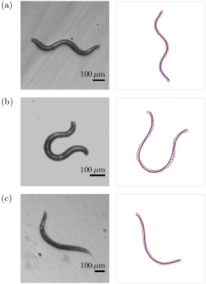
C. elegans propels itself by producing sinuous undulation propagating along the body, Gray and Lissmann (1964) and turns by assuming strongly curved - and loop-shaped body postures.Gray, Hill, and Bargmann (2005) The wavelength of the undulation depends on the environment in which the nematode moves. Crawling on smooth surfaces (such as agar in laboratory experiments), C. elegans assumes short-wave -shaped body postures, and during swimming in water it displays a longer-wave -shaped body form. Using a simple set of body movements, nematodes efficiently maneuver in diverse environments such as soft moist surfaces, bulk and confined fluids, and complex inhomogeneous media. Typical body shapes of C. elegans are illustrated in Fig. 1.
Recent investigations of the response of C. elegans to increased fluid viscosity Korta et al. (2007); Berri et al. (2009); Fang-Yen et al. (2010); Vidal-Gadea et al. (2011) and confinement pressure Lebois et al. (2012) have shown a continuous transition between the long-wave swimming gait in water and a short-wave gait (similar to the crawling gait) in high-viscosity fluids. Understanding of this phenomenon will provide important clues for modeling neural control and biomechanics.
To elucidate this transition, a detailed analysis of hydrodynamics of swimming for a variety of gaits is needed. Using numerical models, this study investigates nematode swimming in different environments. Since experiments are often performed in parallel-wall cells, Jung (2010); Sznitman et al. (2010b); Lebois et al. (2012) we consider swimming in bulk fluids and in fluids confined between two parallel walls. The analysis draws on our recently developed piecewise-harmonic-curvature (PHC) description of worm kinematics. Padmanabhan et al. (2012) As discussed in Sec. II, the PHC model allows us to quantitatively describe nematode shapes used in crawling and swimming. It is also a convenient tool to investigate turns.
In Sec. III we formulate a mobility relation for active-particle locomotion, present our hydrodynamic modeling techniques, and discuss the role of confinement in generating hydrodynamic propulsive force. The results for swimming velocity for different nematode gaits are given in Sec. IV. Our analysis of turning maneuvers presented in Sec. V (to our knowledge the first quantitative study of the hydrodynamics of nematode turns) will have important implications for investigations of nematode chemotaxis. Albrecht and Bargmann (2011)
II Nematode kinematics: piecewise-harmonic-curvature representation of nematode gait


C. elegans move forward by producing sinuous undulations and turn by assuming strongly curved body shapes. The deformations of the nematode body take place in two dimensions, i.e., in the ventral–dorsal plane. The head of the nematode can additionally move normal to this plane, resulting in three-dimensional motion. Here we restrict our analysis to two-dimensional swimming; the effects of normal movements of nematode head will be described elsewhere.
We have recently demonstrated that the gait of crawling and swimming C. elegans can be accurately modeled using a piecewise-harmonic expression for its body curvature. Padmanabhan et al. (2012) This PHC representation applies to individual body shapes (including -shapes, -shapes, and -shapes depicted in Fig. 1) as well as to whole tracks of C. elegans crawling on agar. We have also shown that a similar description applies to swimming C. elegans.
According to the PHC model, the evolution of the body shape is described by the curvature wave propagating along the nematode body,
| (1) |
where is the wave-propagation velocity, is time, and is the coordinate along the nematode body (with and denoting the tail and head positions). The analysis of nematode body postures Padmanabhan et al. (2012) shows that the curvature wave is well represented by the piecewise-harmonic function
| (2) |
with
| (3) |
where are the mode-change points, and , , and are the amplitude, wavevector, and phase of the mode
The real-space curves defined by the curvature can be obtained by solving Frenet–Serret equations
| (4) |
where and are the Cartesian coordinates in the plane of motion, and the dot denotes differentiation with respect to the variable .
According to equation (1), a sequence of nematode’s body postures corresponds to a line section of length sliding with velocity along a curve defined by Eq. (4). In addition to sliding along the curve, a swimming nematode undergoes a rigid-body translational and rotational slip with respect to the surrounding medium. This dynamics is schematically illustrated in Fig. 2.
The family of curves defined by the single-mode relation
| (5) |
with different values of the normalized amplitude is illustrated in Fig. 3. Changing at a fixed value of results in rescaling of the whole curve. Single-mode fits (5) to the nematode shapes depicted in the left panels of Fig. 1 are presented in the corresponding right panels. We note that the shape of a nematode of length at time is described by three dimensionless parameters: the normalized amplitude , dimensionless wavevector , and the phase .
As argued in Ref. Padmanabhan et al., 2012, nematodes use a single mode to move forward and they switch modes in order to turn. Our analysis of rectilinear swimming (see Sec. IV) explores the entire space of the PHC parameters and . We determine the dependence of the normalized swimming velocity on the nematode gait, thus providing important insights regarding the gait transition observed for C. elegans swimming in highly viscous fluids. Korta et al. (2007); Berri et al. (2009); Fang-Yen et al. (2010); Vidal-Gadea et al. (2011) In our discussion of turning maneuvers (see Sec. V) we use a more limited set of parameters, because in a multi-mode system the parameter space is too large to be fully explored. Assuming that the nematode switches from the default -shaped or -shaped forward-locomotion mode [cf. Figs. 1(a) and 1(c)] to -shaped turning mode [cf. Fig. 1(b)] and then reverts to the default mode, we focus on the dependence of the turning angle on the phases at which the PHC modes are switched.
III Nematode hydrodynamics
III.1 Balance of forces and torques acting on the nematode body
In our model, the undulating body of the nematode experiences hydrodynamic forces and torques produced by the propagating wave of PHC. Under creeping flow conditions (assumed herein), the total hydrodynamic force and torque acting on a swimming nematode can be expressed as a superposition of the contribution produced by the predetermined motion with velocity along the line defined by the PHC relation (2) and Frenet–Serret equations (4) [cf. Fig. 2(a)] and the contribution due to the rigid-body translation and rotation with the linear and angular velocities and [cf. Fig. 2(b)]. In the creeping flow regime both these terms are given by the linear friction relations. The total force and torque balance can thus be expressed as
| (6) |
where () are the active-force- and active-torque-generation tensors (with superscript referring to the active contribution), and () are the translational and rotational hydrodynamic resistance tensors. All the above tensors depend on the instantaneous posture of the nematode body. Since the nematode is force- and torque-free,
| (7) |
the friction relation (6) yields the following mobility relation for the rigid-body translation and rotation of an active particle
| (8) |
where
| (9) |
is the mobility matrix for a given nematode posture. In Secs. III.2 and III.3 we describe our methods for evaluating the above matrices using accurate bead-chain models.

III.2 Bead models
To determine the mobility matrix (9) we model the nematode as an active chain of hydrodynamically interacting spheres. The chain performs a set of motions similar to a sequence of body postures of a real nematode [see Fig. 4(a)]. In addition to the translational motion, the beads rotate to mimic deformation of the interface of an elongated body, as illustrated in Fig. 4(b). In more detail, the bead-chain kinematics is described in Appendix A.
For each chain configuration (in our simulations described by the PHC model), the active-force and friction tensors in Eq. (6) are evaluated from the corresponding hydrodynamic-resistance matrix for a system of hydrodynamically coupled spheres. The bead positions are then updated according to the changing chain configuration and the rigid-body velocity (8). In our simulations we use the forth-order Runge–Kutta method for time stepping.
It has been shown that bead-chain models faithfully reproduce hydrodynamic interactions of elongated bodies, Guzowski et al. (2008) so we expect that our calculations accurately describe nematode motion. Details of the chain kinematics and the relevant resistance relations are presented in Appendix A.
We consider a nematode swimming in two distinct geometries: (a) an unbounded fluid and (b) the midplane of a parallel-wall channel. In the first case, the hydrodynamic interactions between the beads representing the nematode body are evaluated using the Hydromultipole method. Cichocki et al. (1994) In the second case we apply the Cartesian-representation (CR) method, Bhattacharya, Bławzdziewicz, and Wajnryb (2005a, b) and we also employ a computationally efficient approximate Hele–Shaw-dipole (HSD) method (see Appendix B).
In our simulations of swimming nematodes we use chains of length beads, consistent with the average thickness-to-length ratio of C. elegans. Bead models allow us to determine effects of finite body thickness and confining walls on the nematode locomotion. These effects are not accounted for in the standard resistive force theory (RFT) Gray and Hancock (1955); Johnson and Brokaw (1979) and slender-body theory (SBT), Johnson (1980); Johnson and Brokaw (1979) and a modified SBT for a confined cylinder between parallel wallsKatz, Blake, and Paveri-Fontana (1975) is inaccurate for geometries relevant for nematode locomotion, as discussed in Sec. III.3.


III.3 Effect of confinement on transverse and longitudinal hydrodynamic forces
Effective undulatory locomotion requires large ratios between the transverse and longitudinal resistance coefficients and that describe friction forces acting on segments of an elongated body. Gray and Hancock (1955); Sauvage et al. (2011) As demonstrated in our earlier studies, Bhattacharya, Bławzdziewicz, and Wajnryb (2005a, b) (also see Refs. Katz, Blake, and Paveri-Fontana, 1975 and Han et al., 2006), the resistance-coefficient ratio is significantly affected by confinement, and can be several times larger in a parallel-wall channel than in an unconfined fluid. Here we show that confinement enhances the efficiency of undulatory swimming as a result of this increased resistance-coefficient ratio.
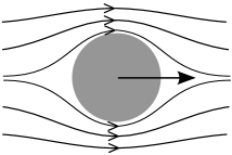
To elucidate the effect of confinement on the propulsion forces in undulatory swimming, we consider the flow field produced by a rigid elongated body in transverse motion through an unconfined fluid and along a flat parallel-wall channel. As schematically illustrated in Fig. 5, an unconfined cylinder produces a long-range flow in the same overall direction as the velocity of the cylinder. The resulting transverse resistance force is relatively low. In the limit of infinite cylinder length, the transverse-to-longitudinal resistance-coefficient ratio logarithmically approaches the asymptotic value , Weinberger (1972); Bławzdziewicz et al. (2005) and for finite cylinders it is even smaller.
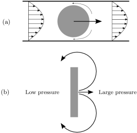
In contrast, for a long cylinder strongly confined between two parallel walls (as shown in Fig. 6) the transverse resistance is significantly larger. This large resistance stems from the pressure distribution needed to drive fluid flow from the region in front of the cylinder to the region behind it. Bhattacharya, Bławzdziewicz, and Wajnryb (2005a, b); Han et al. (2006) For a tightly confined system, the fluid is forced around the ends of the cylinder, as opposed to leaking between the cylinder and the walls [cf. Fig. 6(b)]. Thus the cylinder acts as a piston pushing fluid in the direction parallel to the walls. The parabolic flow produced by this elongated-piston effect occurs over a distance comparable to the cylinder length and thus requires a large pressure drop, producing a large resistance force.
The effect of the above hydrodynamic-friction mechanism on the resistance-coefficient ratio is depicted in Figs. 7 and 8 where we show for submerged linear chains of spheres moving in the midplane of a parallel-wall channel. In Fig. 7 the resistance-coefficient ratio is plotted vs. the chain length for different confinement ratios (where is the channel width and is the bead diameter). Figure 8 depicts the dependence of on for varying chain lengths. In addition, Fig. 8 also compares our bead-chain results with the resistance-coefficient ratio calculated using a modified SBT for a confined cylinder with , where is the cylinder diameter and is the cylinder length. Katz, Blake, and Paveri-Fontana (1975) We find that SBT significantly overpredicts the resistance ratio for the systems considered in our study, most likely due to large logarithmic corrections resulting in a narrow validity range of the approximation.
Our calculations show that, consistent with the elongated-piston mechanism, the resistance-coefficient ratio increases with the increasing chain length. The largest ratio is observed at a dimensionless channel separation of . For tighter confinements the resistance forces are dominated by the lubrication forces between the walls and the particle. The lubrication forces are significantly more isotropic Sauvage et al. (2011) than the forces associated with the piston effect; hence the decrease of the friction-coefficient ratio for . For larger wall separations, more fluid leaks between the particle and walls, which also results in a decrease of . The decrease is gradual: we find that the elongated-piston effect is fairly strong for , and the enhanced transverse resistance is still noticeable even for .
The above results suggest that the effectiveness of nematode swimming is strongly affected by confinement. This conclusion is supported by explicit calculations presented in Sec. IV.
IV Effectiveness of locomotion for different confinements and nematode gaits
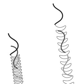


Figure 9 illustrates typical trajectories of a swimming nematode in unconfined (left) and confined (right) fluid. In both cases the nematode uses the same sequence of body motions. Each panel shows the path of the nematode tail and three snapshots of body postures separated by the same phase difference.
Consistent with the discussion in Sec. III.3, the unconfined nematode experiences much more backward slip with respect to the surrounding fluid (compared to the motion with no sidewise slip along the harmonic-curvature path). Hence, the worm is less efficient, i.e., it moves a shorter distance for the same sequence of body postures than the confined nematode. Our numerical results closely resemble trajectories of swimming C. elegans depicted in Fig. 1(a) of Ref. Sznitman et al., 2010b.
In order to quantify the effect of the hydrodynamic slip on the nematode motion, we define the normalized swimming velocity
| (10) |
where denotes the average velocity of the worm, and is the propagation velocity of the curvature wave (1) along the nematode body.
Our results for the normalized velocity (10) for different swimming gaits of confined and unconfined nematodes are presented in Figs. 10–13. The nematode gait is characterized by the dimensionless amplitude (which defines the shapes of the no-slip trajectories represented in Fig. 3), and by the wavevector normalized by the nematode length .
Figures 10 and 11 show the swimming velocity vs. the normalized wavevector in unconfined and confined systems, respectively, for several values of the dimensionless amplitude. The insets in Fig. 10 show the nematode shapes corresponding to characteristic parameter values. Since the parameter ranges in Figs. 10 and 11 are the same, and the maximal efficiency occurs at a similar value of the wavelength , the characteristic shapes shown in Fig. 10 also apply to the results depicted in Fig. 11.
We find that the maximal normalized swimming velocity occurs for a similar amplitude but a shorter wavelength than the wavelength of a typical -shaped body posture of a nematode swimming in water [as depicted in Fig. 1(c)]. The maximum of occurs for , whereas a typical -shaped swimming body posture corresponds to . The wavelength at the maximal velocity is similar to the wavelength of both the -shaped crawling gait [cf., Fig. 1(a)] and gait observed for C. elegans swimming in a high-viscosity fluid. Korta et al. (2007); Berri et al. (2009); Fang-Yen et al. (2010); Vidal-Gadea et al. (2011) Approximate computations using HSD method yield a slightly smaller wavelength value .
Both for unconfined and confined systems the normalized swimming velocity drops sharply for small , because the worm body undergoes only slight deformations for . The normalized velocity also significantly decreases at short wavelength (large ), because of finite thickness effects. For confined worms, there is an additional contribution to this decrease, resulting from a smaller transverse resistance for short coherently moving body segments (consistent with the elongated-piston mechanism described in Sec. III.3). Therefore, the effects of finite thickness of the nematode’s body on the swimming velocity are explored in more detail in Appendix A.
The dependence of on is depicted in Fig. 12. For each value of and channel width, the wavevector corresponds to the maximal value of (cf. Figs. 10 and 11). Figure 12 also shows the normalized velocity (10) for a worm crawling without sideways slip along the trajectories defined by the Frenet–Serret equation (4). We note that even without slip, is smaller than unity, because is the average velocity in the overall direction of motion, whereas is the velocity along the curved nematode path.
Figures 10–13 show that confining a swimming worm in a parallel wall channel significantly affects the normalized swimming velocity. According to the results plotted in Fig. 13, the normalized velocity is the largest for . The peak of is relatively broad, and for an experimentally relevant value , the normalized velocity is only by 25 % smaller than the maximal value (and twice as large as the corresponding result for unconfined fluid, cf. Fig. 12. We note that enhanced swimming velocity has also been theoretically predicted for a cylindrical swimmer in a tube. Felderhof (2010)
The results shown in Figs. 11–13 have been obtained using two complementary methods: the highly accurate but numerically expensive CR method Bhattacharya, Bławzdziewicz, and Wajnryb (2005a, b) and HSD approximation (described in Appendix B), which is much faster and easier to implement. At large wavevectors and high amplitudes of the undulations, the HSD method overpredicts the swimming velocity. However, it yields a good approximation for moderate values of and that are relevant for swimming nematodes.

V Hydrodynamics of Turns


Nematodes navigate their environment by performing a series of turns to move towards the increasing concentration of a chemoattractant Pierce-Shimomura, Dores, and Lockery (2005) or in a direction of a favorable-temperature region.Ryu and Samuel (2002) In our recent paper Padmanabhan et al. (2012) we have shown that the nematode C. elegans turns by abruptly changing the amplitude, wavevector, and phase of the PHC function (1). This behavior was thoroughly documented for a crawling C. elegans, but our additional observations suggest that a similar turning mechanism applies to swimming.
In this paper we consider three-mode turns, where the nematode initially moves using a mode typical of forward locomotion, then increases the amplitude to the -shaped mode [cf. Fig. 1(b)], and finally returns to the initial forward-locomotion mode,
| (11) |
In our calculations we use the normalized amplitude for the default (forward) mode and for the turning mode. The normalized wavevector and phase during the turn remain unchanged.
As illustrated in Fig. 14(a), the turning angle of a nematode crawling without slip depends on purely geometrical factors: the lines corresponding to different modes (11) are smoothly joined together, and the turning angle is obtained as a combination of the line slopes at the joining points. Hence, evaluating the turning angle only requires explicit integration of Eq. (4) with respect to , with the curvature given by Eq. (11). The turning angle depends on the PHC mode parameters (including the points and where the modes switch), but is independent of the normalized wavevector .
For a swimming nematode, the turning angle is affected by the rotational slip of the nematode body with respect to the surrounding medium. The slip depends both on the normalized amplitude and the wavevector of the curvature wave defining the sequence of shapes assumed by the nematode. The magnitude of the rotational slip also depends on the confinement. Hence, all of the above factors influence the turning angle. The evolution of the worm shape is determined by combining Eq. (11) with Eq. (3) relating the spatial variable to time.
Turning maneuvers of unconfined and confined swimming nematodes are illustrated in Fig. 14, both for -shaped and -shaped nematode gaits. As discussed in Sec. IV, the -shaped nematode body [Figs. 14(b) and 14(c)] corresponds, approximately, to the gait for which the normalized swimming velocity assumes the maximal value. This shape is characteristic of nematodes crawling and swimming in high-viscosity fluids. The -shaped body [Figs. 14(d) and 14(e)] corresponds to the gait observed for C. elegans swimming in water, as depicted in Fig. 1(c). The results shown in Fig. 14 indicate that the same sequence of body postures that produces a turn for a nematode crawling without slip yields a similar turn for a swimming nematode. However, the turning angle is smaller, especially for the unconfined nematode.
Figure 15 shows the turning angle vs. the point of initial mode change for two values of the turning-mode length , [with corresponding to a point where has a maximum, according to Eq. (11)]. The dependence of on for two values of is depicted in Fig. 16. The results indicate that the choice of mode change parameters and has a significant effect on the turning angle, both in the sign and magnitude. Confined swimming worms consistently perform sharper turns than their unconfined counterparts. The turning angles of worms employing the -shape and -shape gaits are similar. We find that the differences between turning angles determined using the HSD approximation and CR method (not shown) are small, with a typical errors not exceeding in the domain explored in our simulations.
The results in Fig. 16 are depicted for two periods of the normalized length of the turning mode . For a swimming nematode, the results in the domain are slightly different than in the subsequent periods where , because in the first period the nematode can accommodate all three (i.e., the initial, turning, and final) modes simultaneously along its body. Such three-mode body postures do not occur for the subsequent periods of .
Since the results shown in Fig. 16 indicate that the effect of the three-mode postures on the turning angles is minimal, turning angles can be accurately estimated by combining results for single-mode and two-mode trajectories. Such a simplified approach significantly reduces the size of parameter space needed to fully characterize the turning maneuvers. In our future study of nematode chemotaxis, this simplified method will increase the efficiency of numerical simulations.
VI Conclusions
Combining our PHC description of the nematode gait Padmanabhan et al. (2012) and highly accurate hydrodynamic models, we have quantitatively characterized locomotion capabilities of swimming submillimeter-size nematodes. We have investigated the swimming velocity and turning maneuvers for locomotion in unconfined fluid and in a fluid confined by two parallel walls. The swimming effectiveness was characterized by the swimming velocity normalized by the velocity of curvature wave propagating along the nematode body.
We have determined the dependence of the normalized velocity on the wavevector and amplitude of the curvature wave. It has been found that the velocity is maximal for the normalized amplitude , consistent with our earlier experimental study of the gait of a swimming nematode. Padmanabhan et al. (2012) However, the wavelength of the gait corresponding to the maximal velocity is shorter than the experimentally observed wavelength for nematodes swimming in water. We determined that the calculated wavelength is similar to the one characteristic of a nematode swimming in a high-viscosity fluid. Fang-Yen et al. (2010) In a forthcoming publication we will show that the choice of swimming gait can be explained using energy-dissipation considerations: the gait change stems from a different wavelength dependence of the hydrodynamic energy dissipation in the external fluid and the internal dissipation in the nematode body.
Our numerical simulations of nematodes swimming in a parallel-wall channel reveal that confinement can significantly enhance the swimming velocity. This behavior stems from the increased transverse hydrodynamic resistance due to a large pressure drop across the nematode body moving sideways in a narrow space. We find that for the confinement ratio the normalized swimming velocity exceeds by a factor of two the swimming velocity of an unconfined nematode. The effect of the increased swimming velocity should be taken into account in interpretation of experimental observations of nematode locomotion in parallel-plate cells.
The enhanced swimming velocity under strong confinement in a parallel-wall cell was, in fact, observed in recent experiments. Lebois et al. (2012) Our results provide the explanation of this phenomenon. An increased locomotion efficiency was also seen for C. elegans moving in microfabricated pillar environments. Majmudar et al. (2012); Park et al. (2008) However, in a pillar system C. elegans produces effective propulsion by pushing against mechanical obstacles, whereas the effect described in our study is of purely hydrodynamic origin.
The analysis of turning maneuvers shows that turns in swimming and turns in crawling can be performed using the same set of body postures. The turning angle is larger for a worm crawling without slip, but the angles in swimming are sufficiently large for effective maneuverability. To our knowledge, this study is the first systematic hydrodynamic investigation of turning maneuvers in undulatory locomotion. Results of our hydrodynamic calculations of swimming speed and turning angles have immediate applications in modeling chemotaxis of nematodes immersed in water, Patel et al. (2012) thermotaxis and electrotaxis. We are also using these results to study motor control of a swimming C. elegans.
Acknowledgements.
We would like to acknowledge financial support from NSF Grant No. CBET 1059745 (A. B. and J. B.) and National Science Center (Poland) Grant No. 2012/05/B/ST8/03010 (E. W.). S. A. V. acknowledges NSF CAREER Award Grant No. 1150836.Appendix A Active bead-chain model
In our calculations the body of the nematode is modeled as a long active chain of touching beads. The chain undergoes deformations that mimic undulatory motion of a swimming worm (cf. Fig. 4). The overall translational and rotational motion of the chain results from the balance of the hydrodynamic forces and torques acting on the beads. Chain kinematics is described in Sec. A.1, and chain hydrodynamics is analyzed in Sec. A.2.
A.1 Chain kinematics
Consistent with the description of nematode kinematics introduced in Secs. II and III.1 (see Fig. 2), the beads move along the line defined by the Frenet–Serret equations (4) with the piecewise-harmonic curvature (2). In the lab coordinate system , the line rotates and translates with the linear and angular velocities and . Accordingly, the translational and rotational velocities of each bead,
| (12a) | |||||
| (12b) | |||||
have the active components and associated with the forward motion along the line , and rigid-body components
| (13a) | |||||
| (13b) | |||||
where is the position of the bead .
The active component of the linear velocity of bead is given by the relation
| (14) |
where is the unit vector tangent to the curve at the position of bead . Relation (14) corresponds to the active rod moving along the line with velocity and is fully determined by the system geometry. In contrast, the angular velocities of the beads
| (15) |
(where is the unit vector in the direction normal to the plane of motion), are not uniquely determined, except for a chain moving along a line with constant curvature . In this case the angular velocities of all beads are the same,
| (16) |
because the chain moves along the circle as a rigid body. [For a force-free and torque-free chain submerged in a fluid the velocity component (13) compensates for the imposed motion (15) and (16), so that a circular chain remains at rest.] To verify the accuracy of our approach, we examine three internally consistent bead-rotation models for a flexible chain moving along a line with a varying curvature . We find that at short wavelengths bead rotations have a large effect on the motion of a chain, but the choice of a specific rotation model does not influence the results in a significant way.
Local-curvature model.—
Model with no interparticle slip.—
Bead angular velocities are chosen in such a way that interparticle slip is not present. Accordingly, it is assumed that the angular velocities of the beads satisfy the no-relative-slip condition
| (18) |
where is the angular velocity of the vector connecting beads and , which is computed as
| (19) |
Here denotes the unit vector along the line connecting beads and , and is the unit vector normal to . The system of equations (18) is solved subject to the boundary condition
| (20) |
which ensures the consistency condition (16).
Model with smoothed angular velocity.—
This approach aims to more accurately mimic the motion of deformable interface of the nematode for a system with a strongly nonlinear variation of the curvature. To smooth out the effect of rapid curvature variation, the angular velocity of bead is given as the average rate of rotation of the directors and . Accordingly, the bead angular velocities are given by
| (21) |
The angular velocities of the first and last beads are
| (22) |

The effect of bead rotation on the swimming speed of an active rod is illustrated in Fig. 17. By comparing the results that include consistent bead-rotation models with a calculation that neglects bead rotations entirely, we find that the angular velocities of the beads have a significant effect on the chain velocity. However, if the bead rotations are properly implemented, discrepancies between various rotation models are small, with appreciable differences occurring only in the regime where the wavevector normalized by the bead diameter is too large, . In this regime noticeable differences are expected even for a continuous elongated body, because deformation details are not uniquely determined by the curvature of centerline alone.
In Fig. 17 the results of the bead-chain model are also compared to the normalized swimming velocity evaluated using the RFT with the resistance-coefficient ratio (corresponding to a coherently moving 15-bead chain segment). The results indicate that RFT does not capture the decrease of the swimming velocity at short waves, and therefore significantly overpredicts the normalized swimming velocity in this regime.
A.2 Hydrodynamic interactions
Under creeping-flow conditions, the hydrodynamic force and torque acting on bead in a chain moving through a viscous fluid is related to linear and angular bead velocities via the -particle friction relation
| (23) |
where () are the translational () and rotational () hydrodynamic resistance coefficients.
The total force acting on the chain is equal to the sum of the forces on individual beads
| (24) |
The total torque
| (25) |
includes the sum of individual bead torques as well as the torque due to the forces acting on the beads. Taking into account the velocity decomposition (12), the total force and torque can be represented as a superposition of the active and hydrodynamic-resistance components,
| (26) |
where
| (27) |
and
| (28) |
Combining expressions (23)–(25) with the bead rotation models of Sec. A.1 we find the active-force matrix
| (29) |
(where and are the normalized active linear and angular velocities of the particles), and the chain-resistance hydrodynamic matrix
| (30) |
In the above equations, is the identity tensor, the dagger denotes the transpose, and we use the cross-product operator notation
| (31) |
where is an arbitrary vector. Equations (29) and (30) provide a link between the active bead-chain model and the hydrodynamic description of nematode locomotion given in Eqs. (6)–(9).
For a bead chain moving in an unconfined space, the multiparticle hydrodynamic resistance matrix is evaluated using the Hydromultipole method. Cichocki et al. (1994) For a parallel-wall geometry we use the CR method. Bhattacharya, Bławzdziewicz, and Wajnryb (2005a, b) In both cases, the lubrication resistance for touching neighboring beads is truncated at a finite gapwidth between particle surfaces. This truncation allows us to avoid infinite internal friction in the chain. The active force and resistance coefficients (27) and (30) are non-singular in the limit . We find that the numerical results for chain motion are insensitive to the value of for .
Evaluation of the hydrodynamic-interaction tensors using the CR method is very accurate but numerically expensive. Thus we have also developed a less accurate but much faster Hele–Shaw dipole (HSD) approximation, described in Appendix B. A comparison of HSD results with the CR method, presented in Fig. 11, shows that the HSD approximation provides accurate description of the hydrodynamics of active bead chains at sufficiently long wavelengths.

Appendix B Hele–Shaw dipole approximation
B.1 Interparticle dipolar interactions
An isolated spherical particle in the midplane of a parallel-wall channel, moving with the velocity and subject to the external pressure gradient experiences the hydrodynamic traction force and produces the far-field scattered parabolic flow driven by a two-dimensional pressure dipole, Cui et al. (2004); Bhattacharya, Bławzdziewicz, and Wajnryb (2005b, 2006); Bławzdziewicz and Wajnryb (2008); Janssen et al. (2012)
| (32) |
Here is the lateral position of the field point relative to the lateral particle position , , and is the dipolar moment of the induced pressure dipole. The hydrodynamic traction force and dipolar moment are linearly related to the particle velocity and the external pressure gradient at the particle position,
| (33) |
(where it is assumed that depends only on the lateral coordinates). As discussed in Ref. Bławzdziewicz and Wajnryb, 2008, the force and dipolar moment can be expressed by the generalized resistance relation
| (34) |
where the scalar resistance coefficients depend on the confinement ratio .
In the HSD approximation it is assumed that the particles interact solely via the Hele-Shaw dipolar fields (32). It follows that the flow incident to particle is driven by the pressure gradient
| (35) |
resulting from the superposition of dipolar pressures (32) produced by other particles. By combining Eqs. (34) and (35), we obtain the relations
| (36a) | |||||
| (36b) | |||||
where
| (37) |
is the dipolar-interaction tensor obtained by taking the gradient of Eq. (32).
Eliminating the dipole moment from equations (36) yields the -particle friction relation
| (38) |
in the HSD approximation. The hydrodynamic resistance tensor can be expressed using the -particle matrix relation,
| (39) |
where and are matrices with elements and (), and is the identity matrix in the -particle space.
In the HSD approximation, the dynamics of the active chain is described by the active-force and chain-resistance relations (29) and (30) with
| (40a) | |||
| for the translational components of the -particle hydrodynamic resistance matrix, and | |||
| (40b) | |||
for the components that involve particle rotation. The rotational components (40b) are neglected in the HSD approximation, because particle rotation in the midplane of the channel does not produce far-field dipolar scattered flow.Bławzdziewicz and Wajnryb (2008) However, we expect that incorporating short-range rotational effects in future implementations of the HSD method may improve its accuracy at short wavelengths.
B.2 Application to a system of touching spheres
According to Eq. (39), the HSD approximation involves three independent numerical coefficients, i.e., , , and the product , which describe the single-particle hydrodynamic response (34) of a particle to its translational motion and to the applied pressure gradient. When the values corresponding to the dynamics of an isolated particle are used for these coefficients, an asymptotic approximation for a system of widely separated particles is obtained. Such an approximation, however, is inaccurate if the interparticle distance is comparable to the channel width. Baron, Bławzdziewicz, and Wajnryb (2008)
In the present study the HSD approximation is applied outside the far-field asymptotic regime. Therefore, we use an alternative approach, where we treat the coefficients , , and as adjustable parameters. The values of these parameters are determined by fitting the HSD results to accurate CR calculations for the resistance coefficients of rigid linear chains of touching spheres. The same values are then used in our simulations of the motion of active particle chains.
For a given normalized channel width , the optimal parameter values are determined by minimizing the fitting error
| (41) |
where and are the lateral and transverse resistance coefficients of chains of different lengths . The indices CR and HSD refer to the results obtained using the CR algorithm Bhattacharya, Bławzdziewicz, and Wajnryb (2005a, b) and HSD approximation (39), respectively.
| 1.01 | 0.85223 | 0.05176 | 0.15010 |
| 1.02 | 0.82923 | 0.05748 | 0.15001 |
| 1.03 | 0.80829 | 0.06030 | 0.15032 |
| 1.04 | 0.79819 | 0.06347 | 0.15003 |
| 1.05 | 0.78857 | 0.06559 | 0.14990 |
| 1.06 | 0.78352 | 0.06726 | 0.14976 |
| 1.07 | 0.78188 | 0.06910 | 0.14945 |
| 1.08 | 0.76290 | 0.06866 | 0.14994 |
| 1.09 | 0.76152 | 0.07058 | 0.14948 |
| 1.1 | 0.75416 | 0.07068 | 0.14960 |
| 1.2 | 0.70692 | 0739421 | 0.14838 |
| 1.3 | 0.67887 | 0.07304 | 0.14705 |
| 1.4 | 0.65012 | 0.07020 | 0.14570 |
| 1.5 | 0.64069 | 0.06973 | 0.14323 |
| 2.0 | 0.56027 | 0.05441 | 0.13770 |
| 2.5 | 0.52446 | 0.04719 | 0.13036 |
| 3.0 | 0.48439 | 0.03928 | 0.12826 |
In our calculations we have used the summation range from to and the value for the weight of the lateral resistance component relative to the transverse component. The lower summation limit corresponds to the chain length below which the HSD approximation is not expected to hold, based on the decay distance of the near-field contributions. Bhattacharya, Bławzdziewicz, and Wajnryb (2006); Baron, Bławzdziewicz, and Wajnryb (2008) The upper limit is the chain length used in our simulation of nematode locomotion. The fitting error (41) was minimized using the conjugate-gradient method.
The results of our calculations are illustrated in Fig. 18, where we compare HSD approximation with accurate results obtained using the CR method. For sufficiently large chain lengths , the HSD approximation agrees well with the accurate calculations, especially for narrow channels. The error for the resistance-coefficient ratio is small in the whole range of chain lengths , as depicted in Fig. 18(c). The optimal values for the coefficients , , and the product for different channel widths are listed in Table 1.
The above fitting procedure optimizes the accuracy of the resistance coefficients for linear chains of spheres. Since the motion of deformable active chains is determined by hydrodynamic interactions of coherently moving chain segments, the HSD approximation yields accurate results for active chains at sufficiently long wavelengths.
References
- Lauga and Powers (2009) E. Lauga and T. R. Powers, “The hydrodynamics of swimming microorganisms,” Rep. Prog. Phys. 72, 096601 (2009).
- Cohen and Boyle (2010) N. Cohen and J. Boyle, “Swimming at low Reynolds number: a beginners guide to undulatory locomotion,” Contemp. Phys. 51, 103–123 (2010).
- Metcalfe and Pedley (2001) A. M. Metcalfe and T. J. Pedley, “Falling plumes in bacterial bioconvection,” J. Fluid Mech. 445, 121–149 (2001).
- Juarez et al. (2010) G. Juarez, K. Lu, J. Sznitman, and P. Arratia, “Motility of small nematodes in wet granular media,” EPL 92, 44002 (2010).
- Jung (2010) S. Jung, “Caenorhabditis elegans swimming in a saturated particulate system,” Phys. Fluids 22, 031903 (2010).
- Sauvage et al. (2011) P. Sauvage, M. Argentina, J. Drappier, T. Senden, J. Siméon, and J.-M. Di Meglio, “An elasto-hydrodynamical model of friction for the locomotion of Caenorhabditis elegans,” J. Biomech. 44, 1117 (2011).
- Majmudar et al. (2012) T. Majmudar, E. E. Keaveny, J. Zhang, and M. J. Shelley, “Experiments and theory of undulatory locomotion in a simple structured medium,” J. R. Soc. Interface. 9, 1809–1823 (2012).
- Guasto, Rusconi, and Stocker (2012) J. S. Guasto, R. Rusconi, and R. Stocker, “Fluid mechanics of planktonic microorganisms,” Annu. Rev. Fluid Mech. 44, 373–400 (2012).
- Wu and Libchaber (2000) X. L. Wu and A. Libchaber, “Particle diffusion in a quasi-two-dimensional bacterial bath,” Phys. Rev. Lett. 84, 3017–3020 (2000).
- Hernández-Ortiz, Stoltz, and Graham (2005) J. P. Hernández-Ortiz, C. G. Stoltz, and M. D. Graham, “Transport and collective dynamics in suspensions of confined swimming particles,” Phys. Rev. Lett. 95, 204501 (2005).
- Underhill, Hernandez-Ortiz, and Graham (2008) P. T. Underhill, J. P. Hernandez-Ortiz, and M. D. Graham, “Diffusion and spatial correlations in suspensions of swimming particles,” Phys. Rev. Lett. 100 (2008).
- Koch and Subramanian (2011) D. L. Koch and G. Subramanian, “Collective hydrodynamics of swimming microorganisms: living fluids,” Annu. Rev. Fluid Mech. 43, 637–659 (2011).
- Pratt and Kolter (1998) L. A. Pratt and R. Kolter, “Genetic analysis of Escherichia coli biofilm formation: roles of flagella, motility, chemotaxis and type I pili,” Mol. Microbiol. 30, 285–293 (1998).
- Hosoi and Lauga (2010) A. E. Hosoi and E. Lauga, “Mechanical aspects of biological locomotion,” Exp. Mech. 50, 1259–1261 (2010).
- Zhang et al. (2009) L. Zhang, J. J. Abbott, L. Dong, B. E. Kratochvil, D. Bell, and B. J. Nelson, “Artificial bacterial flagella: Fabrication and magnetic control,” App. Phys. Lett. 94 (2009).
- Dreyfus et al. (2005) R. Dreyfus, J. Baudry, M. L. Roper, M. Fermigier, H. A. Stone, and J. Bibette, “Microscopic artificial swimmers,” Nature 437, 862–865 (2005).
- Ahmed, Shimizu, and Stocker (2010) T. Ahmed, T. S. Shimizu, and R. Stocker, “Microfluidics for bacterial chemotaxis,” Integr. Biol. 2, 604–629 (2010).
- Ma et al. (2009) H. Ma, L. Jiang, W. Shi, J. Qin, and B. Lin, “A programmable microvalve-based microfluidic array for characterization of neurotoxin-induced responses of individual C. elegans,” Biomicrofluidics 3, 044114 (2009).
- Chung, Crane, and Lu (2008) K. Chung, M. Crane, and H. Lu, “Automated on-chip rapid microscopy, phenotyping and sorting of C. elegans,” Nat. Methods 5, 637–643 (2008).
- Chronis, Zimmer, and Bargmann (2007) N. Chronis, M. Zimmer, and C. Bargmann, “Microfluidics for in vivo imaging of neuronal and behavioral activity in Caenorhabditis elegans,” Nat. Methods 4, 727–731 (2007).
- Lockery et al. (2008) S. Lockery, K. Lawton, J. Doll, S. Faumont, S. Coulthard, T. Thiele, N. Chronis, K. McCormick, M. Goodman, and B. Pruitt, “Artificial dirt: Microfluidic substrates for nematode neurobiology and behavior,” J. Neurophysiol. 99, 3136–3143 (2008).
- Sznitman et al. (2010a) J. Sznitman, X. Shen, P. K. Purohit, R. Sznitman, and P. E. Arratia, “Swimming behavior of the nematode Caenorhabditis elegans: Bridging Small-Scale Locomotion with Biomechanics,” IFMBE Proc. 31, 29–32 (2010a).
- Sznitman et al. (2010b) J. Sznitman, X. Shen, R. Sznitman, and P. Arratia, “Propulsive force measurements and flow behavior of undulatory swimmers at low Reynolds number,” Phys. Fluids 22, 12901 (2010b).
- Korta et al. (2007) J. Korta, D. Clark, C. Gabel, L. Mahadevan, and A. Samuel, “Mechanosensation and mechanical load modulate the locomotory gait of swimming C-elegans,” J. Exp. Biol. 210, 2383–2389 (2007).
- Berri et al. (2009) S. Berri, J. H. Boyle, M. Tassieri, I. Hope, and N. Cohen, “Forward locomotion of the nematode C. elegans is achieved through modulation of a single gait,” HFSP J 3, 186–93 (2009).
- Fang-Yen et al. (2010) C. Fang-Yen, M. Wyart, J. Xie, R. Kawai, T. Kodger, S. Chen, Q. Wen, and A. D. T. Samuel, “Biomechanical analysis of gait adaptation in the nematode Caenorhabditis elegans,” Proc. Natl. Acad. Sci. U.S.A. 107, 20323–8 (2010).
- Berman et al. (2013) R. S. Berman, O. Kenneth, J. Sznitman, and A. M. Leshansky, “Undulatory locomotion of finite filaments: lessons from C. elegans,” New J. Phys. in review (2013).
- Etheridge et al. (2012) T. Etheridge, E. A. Oczypok, S. Lehmann, B. D. Fields, F. Shephard, L. A. Jacobson, and N. J. Szewczyk, “Calpains mediate integrin attachment complex maintenance of adult muscle in Caenorhabditis elegans,” PLoS. Genet. 8 (2012).
- Omura et al. (2012) D. T. Omura, D. A. Clark, A. D. T. Samuel, and H. R. Horvitz, “Dopamine signaling is essential for precise rates of locomotion by C. elegans,” PLoS ONE 7 (2012).
- Ward et al. (2009) A. Ward, V. J. Walker, Z. Feng, and X. Z. S. Xu, “Cocaine modulates locomotion behavior in C. elegans,” PLoS ONE 4 (2009).
- Downes et al. (2012) J. C. Downes, B. Birsoy, K. C. Chipman, and J. H. Rothman, “Handedness of a motor program in C. elegans is independent of left-right body asymmetry,” PLoS ONE 7, e52138 (2012).
- McCormick et al. (2011) K. E. McCormick, B. E. Gaertner, M. Sottile, P. C. Phillips, and S. R. Lockery, “Microfluidic devices for analysis of spatial orientation behaviors in semi-restrained Caenorhabditis elegans,” PLoS ONE 6 (2011).
- Gray, Hill, and Bargmann (2005) J. Gray, J. Hill, and C. Bargmann, “A circuit for navigation in Caenorhabditis elegans,” Proc. Natl. Acad. Sci. U.S.A. 102, 3184–3191 (2005).
- Artal-Sanz and Tavernarakis (2011) L. Artal-Sanz, M.and de Jong and N. Tavernarakis, “Caenorhabditis elegans: A versatile platform for drug discovery,” J. Biotechnol. 8, 599–U120 (2011).
- Gray and Lissmann (1964) J. Gray and H. Lissmann, “Locomotion of Nematodes,” J. Exp. Biol. 41, 135–54 (1964).
- Padmanabhan et al. (2012) V. Padmanabhan, Z. S. Khan, D. E. Solomon, A. Armstrong, K. P. Rumbaugh, S. A. Vanapalli, and J. Blawzdziewicz, “Locomotion of C. elegans: a piecewise-harmonic curvature representation of nematode behavior,” PLoS ONE 7, e40121 (2012).
- Vidal-Gadea et al. (2011) A. Vidal-Gadea, S. Topper, L. Young, A. Crisp, L. Kressin, E. Elbel, T. Maples, M. Brauner, K. Erbguth, A. Axelrod, A. Gottschalk, D. Siegel, and J. T. Pierce-Shimomura, “Caenorhabditis elegans selects distinct crawling and swimming gaits via dopamine and serotonin,” Proc. Natl. Acad. Sci. U.S.A. 108, 17504–17509 (2011).
- Lebois et al. (2012) F. Lebois, P. Sauvage, C. Py, O. Cardoso, B. Ladoux, P. Hersen, and J.-M. Di Meglio, “Locomotion control of Caenorhabditis elegans through confinement,” Biophys. J. 102, 2791–2798 (2012).
- Albrecht and Bargmann (2011) D. R. Albrecht and C. I. Bargmann, “High-content behavioral analysis of Caenorhabditis elegans in precise spatiotemporal chemical environments,” Nat. Methods. 8, 599–U120 (2011).
- Guzowski et al. (2008) J. Guzowski, B. Cichocki, E. Wajnryb, and G. C. Abade, “The short-time self-diffusion coefficient of a sphere in a suspension of rigid rods,” J. Chem. Phys. 128 (2008), 10.1063/1.2837296.
- Cichocki et al. (1994) B. Cichocki, B. U. Felderhof, K. Hinsen, E. Wajnryb, and J. Bławzdziewicz, “Friction and mobility of many spheres in Stokes flow,” J. Chem. Phys. 100, 3780–3790 (1994).
- Bhattacharya, Bławzdziewicz, and Wajnryb (2005a) S. Bhattacharya, J. Bławzdziewicz, and E. Wajnryb, “Many-particle hydrodynamic interactions in parallel-wall geometry: Cartesian-representation method,” Physica A 356, 294–340 (2005a).
- Bhattacharya, Bławzdziewicz, and Wajnryb (2005b) S. Bhattacharya, J. Bławzdziewicz, and E. Wajnryb, “Hydrodynamic interactions of spherical particles in suspensions confined between two planar walls,” J. Fluid Mech. 541, 263–292 (2005b).
- Gray and Hancock (1955) J. Gray and G. J. Hancock, “The propulsion of sea-urchin spermatozoa,” J. Exp. Biol. 32, 802–814 (1955).
- Johnson and Brokaw (1979) R. E. Johnson and C. J. Brokaw, “Flagellar hydrodynamics. A comparison between resistive-force theory and slender-body theory.” Biophys. J. 25, 113–127 (1979).
- Johnson (1980) R. E. Johnson, “An improved slender-body theory for Stokes flow,” J. Fluid Mech. 99, 411–431 (1980).
- Katz, Blake, and Paveri-Fontana (1975) D. Katz, J. Blake, and S. Paveri-Fontana, “On the movement of slender bodies near plane boundaries at low Reynolds number,” J. Fluid Mech. 72, 529–540 (1975).
- Han et al. (2006) Y. Han, A. Alsayed, M. Nobili, J. Zhang, T. C. Lubensky, and A. G. Yodh, “Brownian motion of an ellipsoid,” Science 314, 626–630 (2006).
- Weinberger (1972) H. F. Weinberger, “Variational properties of steady fall in Stokes flow,” J. Fluid Mech. 52, 321–44 (1972).
- Bławzdziewicz et al. (2005) J. Bławzdziewicz, E. Wajnryb, J. A. Given, and J. B. Hubbard, “Sharp scalar and tensor bounds on the hydrodynamic friction and mobility of arbitrarily shaped bodies in Stokes flow,” Phys. Fluids 17, 033602–1–9 (2005).
- Felderhof (2010) B. U. Felderhof, “Swimming at low Reynolds number of a cylindrical body in a circular tube,” Phys. Fluids 22 (2010).
- Pierce-Shimomura, Dores, and Lockery (2005) J. Pierce-Shimomura, M. Dores, and S. Lockery, “Analysis of the effects of turning bias on chemotaxis in C. elegans,” J. Exp. Biol. 208, 4727–4733 (2005).
- Ryu and Samuel (2002) W. S. Ryu and A. D. T. Samuel, “Thermotaxis in Caenorhabditis elegans analyzed by measuring responses to defined thermal stimuli,” J. Neurosci. 22, 5727–5733 (2002).
- Park et al. (2008) S. Park, H. Hwang, S. W. Nam, F. Martinez, R. H. Austin, and W. S. Ryu, “Enhanced Caenorhabditis elegans locomotion in a structured microfluidic environment,” PLoS One 3, e2550 (2008).
- Patel et al. (2012) A. Patel, A. Bilbao, V. Padmanabhan, Z. S. Khan, A. Armstrong, K. P. Rumbaugh, S. A. Vanapalli, and J. Blawzdziewicz, “Chemotaxis of crawling and swimming Caenorhabditis elegans,” Bul. Am. Phys. Soc. 57(17), H17.00008 (2012).
- Cui et al. (2004) B. Cui, H. Diamant, B. Lin, and S. A. Rice, “Anomalous hydrodynamic interaction in a quasi-two-dimensional suspension,” Phys. Rev. Lett. 92, 258301–1–4 (2004).
- Bhattacharya, Bławzdziewicz, and Wajnryb (2006) S. Bhattacharya, J. Bławzdziewicz, and E. Wajnryb, “Far-field approximation for hydrodynamic interactions in parallel-wall geometry,” J. Comput. Phys. 212, 718–738 (2006).
- Bławzdziewicz and Wajnryb (2008) J. Bławzdziewicz and E. Wajnryb, “An analysis of the far-field response to external forcing of a suspension in Stokes flow in a parallel-wall channel,” Phys. Fluids. 20, 093303 (2008).
- Janssen et al. (2012) P. J. A. Janssen, M. D. Baron, P. D. Anderson, J. Blawzdziewicz, M. Loewenberg, and E. Wajnryb, “Collective dynamics of confined rigid spheres and deformable drops,” Soft Matter 8, 7495–7506 (2012).
- Baron, Bławzdziewicz, and Wajnryb (2008) M. Baron, J. Bławzdziewicz, and E. Wajnryb, “Hydrodynamic crystals: collective dynamics of regular arrays of spherical particles in a parallel-wall channel,” Phys. Rev. Lett. 100, 174502 (2008).