Seeing about Soil – Management Lessons from a Simple Model for Renewable Resources

Abstract

Employing an effective cellular automata model, we investigate and analyze the build-up and erosion of soil. Depending on the strategy employed for handling agricultural production, in many cases we find a critical dependence on the prescribed production target, with a sharp transition between stable production and complete breakdown of the system.

Strategies which are particularly well-suited for mimicking real-world management approaches can produce almost cyclic behaviour, which can also either lead to sustainable production or to breakdown.

While designed to describe the dynamics of soil evolution, this model is quite general and may also be useful as a model for other renewable resources and may even be employed in other disciplines like psychology.
Keywords: cellular automata, renewable resources, management strategies, erosion, critical behaviour
PACS Nos.: 64.60.Ht, 89.60.Gg, 89.75.Fb, 92.40.Gc

1 Introduction

At present, a large part of our economy is built on the exploitation of nonrenewable resources as, for instance, oil, coal and natural gas. It is common sense that we have to put more emphasis on the use of renewable resources, as the amount of nonrenewable resources is strictly limited [1, 2]. Even before these limits are reached, the technological and economic effort of exploitation rises dramatically and ecological consequences tend to become unacceptably severe.

Thus a fundamental change in our behaviour will be necessary in order to avoid catastrophic breakdowns as well as ecological disasters. But also resources which are renewable can still be ruined by overexploitation, with well-known examples for this being overfishing and deforestation.

A particularly important resource both for natural systems and for agriculture is soil. The loss of soil is a topic intensively discussed in recent years, and loss of soil has been made responsible for the breakdown of whole civilizations [3]. Apart from the obvious importance for plant growth, soil is an important ecosystem by itself and one of the largest reservoirs of biodiversity. Unbalanced soil ecology is assumed to be a key factor for the spread of several diseases [4]. In addition, soil can contain large amounts of carbon and building up soil can be a very efficient strategy to capture carbon and remove it from the atmosphere, thus slowing down climate change.

Soil quality, build-up and loss are a topic of intense research, but the mathematical models employed so far tend to be either very simple (for sake of being analytically tractable) or already very specific, including complex chemical and biochemical reactions and connections [5, 6, 7].

In this article we propose an alternative model which captures the main elements of soil evolution. This model exhibits complex behaviour (including critical transitions) but is, at the same time, simple enough to be easily applied also to other renewable resources. For these reasons it can serve as a testing ground for various management strategies.

2 The Model

The present model had initially been built to supplement a climate model presented in [8] with a qualitative description of the interplay of soil and plant life, in particular regarding carbon storage capacity.

Soon it turned out that already without being coupled to the climate model, the plant-soil system revealed dynamics well worth of separate investigation, and it became the topic of the present article.

2.1 Basic Concept

The main ideas behind the model are:

• Natural vegetation builds up soil.

• Natural vegetation is replaced by agricultural fields, depending on a prescribed production goal and the chosen management strategy.

• In agricultural fields, soil is lost due to intense agriculture, and below a certain threshold of soil, agricultural production starts to decline.

In a rather simplified approach to natural succession, we introduce two kinds of plant population:

• Pioneer plants build up soil slowly, but they are able to inhabit even “empty” cells (i.e. those without soil) and spread randomly.

• Forests build up soil faster, but they require a certain soil threshold $\tau_{\rm for}$ to grow at all. In addition, forests can (except in the case of deliberate reforestation, as discussed in sec. 2.2.4) only grow if at least one neighbor cell is also inhabited by forests.

Different strategies for creating and abandoning agricultural fields can be employed in order to fulfill the prescribed production goal, see sec. 2.2.4.

2.2 Implementation

The model is implemented by means of extended stochastic cellular automata [9, 10]. We define the system on a grid, with states conveniently represented by two matrices:

• The inhabitance state of the cells is described by the matrix $\boldsymbol{P}(n_{t})$ with entries $p_{ij}(n_{t})\in\{0,\,1,\,2,\,3\}$, where we use the following assignment:

  1. Cell is uninhabited.

  2. Cell inhabited by pioneer plants

  3. Cell inhabited by forest

  4. Cell used for agriculture

• The amount of soil contained in the cells is described by the matrix $\boldsymbol{S}(n_{t})$ with entries $s_{ij}(n_{t})\in\mathbb{R}_{0}^{+}$.

The parameters of the model are summarized in table 1.

symbol	range	meaning/definition
$N_{1}$	$\in\mathbb{N}$	size of grid (number of cells) in first direction
$N_{2}$	$\in\mathbb{N}$	size of grid (number of cells) in second direction
$N_{t}$	$\in\mathbb{N}$	total number of timesteps
$\rho_{\text{for}}^{\text{(ini)}}$	$\in[0,1]$	initial density of forests (before placing fields)
$\rho_{\text{pio}}^{\text{(ini)}}$	$\in[0,1]$	initial density of pioneer plants
$A^{(\rm goal)}$	$\in[0,\,N_{1}N_{2}]$	goal for agricultural production
$\gamma_{\rm agr}$	$\in[0,1]$	normalized production goal, $\gamma_{\rm agr}=\frac{A^{(\rm goal)}}{N_{1}N_{2}}$
$p_{\text{pio}}$	$\in[0,1]$	probability of an empty cell to become populated by pioneer plants
$\tau_{\text{for}}$	$\in\mathbb{R}^{+}$	soil threshold for forest growth
$\tau_{\rm agri}$	$\in\mathbb{R}^{+}$	soil threshold for decline of agricultural production
$s^{(+)}_{(\text{pio})}$	$\in\mathbb{R}^{+}$	soil build-up per timestep by pioneer plants
$s^{(+)}_{(\text{for})}$	$\in\mathbb{R}^{+}$	soil build-up per timestep by forest
$s^{(-)}_{(\text{agr})}$	$\in\mathbb{R}^{+}$	soil loss per timestep due to agriculture

Table 1: List of parameters employed in the model

2.2.1 Initialization

The grid initalization is done in four consecutive steps, which set up the matrices $\boldsymbol{P}(0)$ and $\boldsymbol{S}(0)$:

1. Forests, described by $p_{ij}(0)=2$, are distributed in the matrix $\boldsymbol{P}(0)$ with the initial forest density $\rho_{\text{for}}^{\text{(ini)}}$.

2. Soil values are determined according to

   $$s_{ij}(0)=\tau_{\text{for}}\,\left(\delta_{2,p_{ij}(0)}+u_{ij}\right)$$ (1)

   with $\delta_{k\ell}$ denoting the Kronecker delta and $u_{ij}$ taken randomly from a uniform $[0,\,1]$-distribution.

3. Agricultural fields are placed employing one of the strategies described in sec. 2.2.4, possibly making use of the information contained in $\boldsymbol{S}(0)$. Note that this will typically reduce the density of forest below the initial value $\rho_{\text{for}}^{\text{(ini)}}$.

4. Of the remaining cells with $p_{i,j}(0)=0$, a fraction of $\rho_{\text{pio}}^{\text{(ini)}}$ is populated with pioneer plants, $p_{i,j}(0)\to 1$.

The target number of agricultural cells is initialized as $N_{\text{agr}}=A^{(\rm goal)}$.

2.2.2 Update Rules

At each time update $n_{t}\to n_{t}+1$ the following update rules are executed:

• According to the re-population probability $p_{\text{pio}}$, empty cells are populated with pioneer plants.

• Any cell $(i,j)$ which is either empty or populated with pioneers is converted to forest with probability

  $$p=\frac{\text{number of neighbouring forest cells}}{\text{total number of neighbour cells}}$$ (2)

  if the condition $s_{ij}(n_{t})\geq\tau_{\text{for}}$ is met. Neighbourhood is defined as a mixed von Neumann-Moore type, with diagonal neighbours carrying half the weight of directly adjacent ones. (In terms of [11], this is implemented by setting $\pi_{\rm M}=\frac{1}{2}$.)

• Agricultural fields are created or abandoned according to the current management strategy, as described in sec. 2.2.4.

• The agricultural production $A(n_{t})$ is calculated as decribed in 2.2.3 and the new target number $N_{\text{agr}}$ is determined according to chosen strategy, based on the relation between production $A(n_{t})$ and production goal $A^{(\rm goal)}$.

• Soil content is modified according to the current cell population,

  $$\delta s(n_{t}) =s^{(+)}_{(\text{pio})}\delta_{1,p_{ij}(n_{t})}+s^{(+)}_{(\text{for})}\delta_{2,p_{ij}(n_{t})}-s^{(-)}_{(\text{agr})}\delta_{3,p_{ij}(n_{t})},$$ (3)

  $$s_{ij}(n_{t}+1) =\max\left(0,s_{ij}(n_{t})+\delta s(n_{t})\right),$$ (4)

  which model soil generation and erosion.

• Cells with $s_{ij}(n_{t})=0$ become empty, $p_{ij}(n_{t}+1)=0$.

2.2.3 Determining Agricultural Production

The agricultural production $a$ of an appropriate cell $(i,\,j)$ during timestep $n_{t}$ is equal to a constant $a_{0}$ as long as the amount of soil is above a fixed threshold, $s_{ij}(n_{t})\geq\tau_{\rm agri}$. If $s_{ij}(n_{t})<\tau_{\rm agri}$, we assume direct proportionality of production to the amount of soil, with a continuous transition between the two regimes. The constant $a_{0}$ can be chosen equal to one, which normalizes the production and thus sets the scale. This yields

$$a(i,j,n_{t})=\frac{\delta_{3,p_{i,j}(n_{t})}}{\tau_{\rm agri}}\,\min\left(s_{ij}(n_{t}),\,\tau_{\rm agri}\right).$$ (5)

The total production is obtained as

$$A(n_{t})=A(\boldsymbol{P},\boldsymbol{S},n_{t})=\sum_{i,j}a(i,j,n_{t}).$$ (6)

2.2.4 Resource Management Strategies

The most intricate component of the model is the strategy how to handle the agricultural fields. A multitude of strategies is possible, of which we have chosen a small subset which is relatively easy to describe and to implement.

All strategies studied in this article are based on four basic ways to handle the distribution of agricultural cells, which for brevity are denoted as ”fields”:

1. Keep fields as long as possible

2. Abandon fields as soon as soil drops below agricultural threshold

3. Redistribute fields at each step, no reforestation

4. Redistribute fields at each step, reforestation if possible

Reforestation is the only way how a cell can be populated with forest without having a neighbour forest cell. Reforestation of a cell $(i,j)$ only succeeds if $s_{ij}(n_{t})\geq\tau_{\rm for}$. These basic strategies have been combined with two ways how cells are chosen as new fields:

• Choose new fields randomly: ${}_{\text{rand}}$,

• Choose new fields according to maximum soil: ${}_{\text{opt}}$

In addition we compare two ways how to handle the number of agricultural fields:

• Number of fields is held fixed: ${}^{\text{(fix)}}$,

• Number of fields is variable: ${}^{\text{(var)}}$

In the present simulation, for ${}^{\text{(var)}}$ we have employed the strategy to raise the number of fields by $1\%$, if during the last timestep the production was below the production goal, $A(n_{t}-1)<A^{(\rm goal)}$ and abandon $1\%$ of the fields if $A(n_{t}-1)>A^{(\rm goal)}$. The rate of $1\%$ per timestep is arbitrary, but it at least qualitiatively captures the inertia effects induced by the effort of establishing new fields and by the reluctance of abandoning existing ones.

Combinatorics yields sixteen different strategies how to manage agricultural production within this model. For example strategy $\text{[S1]}_{\text{rand}}^{\text{(fix)}}$ would keep fields as long as possible, but keep the number of fields fixed. With this strategy certain drops in productivity are unavoidable within this model.

In sec. 4 it will turn out that depending on the production goal, the same principal strategy can yield dramatically different results.

3 Sample Runs and Methods of Data Analysis

A typical sample run for the model, employing strategy $\text{[S1]}_{\text{rand}}^{\text{(fix)}}$ and standard parameters as given in table 2, is shown in fig. 1.a.

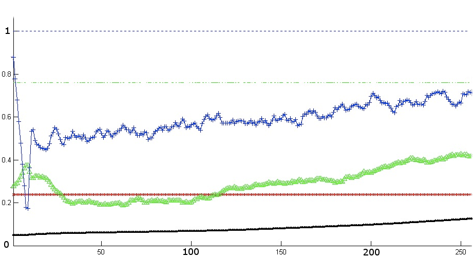
Figure 1: Influence of production target on simulation results, illustrated by sample simulation runs. For these runs, strategy $\text{[S1]}_{\text{rand}}^{\text{(fix)}}$ has been employed with (a) $\gamma_{\rm agr}=0.24$ and (b) $\gamma_{\rm agr}=0.25$.
Other parameters have been set to standard values as given in tab. 2.
We plot the following quantities as function of the time step index $n_{t}$:

	density of agricultural cells,
	minimum possible density of agricultural cells,
	density of forest cells,
	maximum possible density of forest cells,
	normalized agricultural production,
	normalized target agricultural production (equal to one),
	amount of soil, displayed on a linear-logarithmic scale (see eq. (11)).

The plot shows the density of agricultural cells

$$\rho_{\text{agr}}(n_{t})=\frac{1}{N_{1}N_{2}}\sum_{i,j}\delta_{3,p_{ij}(n_{t})},$$ (7)

(which is constant in this case), the density of trees

$$\rho_{\text{for}}=\frac{1}{N_{1}N_{2}}\sum_{i,j}\delta_{2,p_{ij}(n_{t})},$$ (8)

the normalized agricultural production

$$a(n_{t})=\frac{A(n_{t})}{A^{(\rm goal)}}$$ (9)

and a measure for the amount of soil. Since the average amount of soil can grow very large in this model, we do not directly plot the normalized amount of soil

$$s(n_{t})=\frac{1}{N_{1}N_{2}}\sum_{i,j}s_{ij}(n_{t}),$$ (10)

but instead show the quantity

$$\tilde{s}(n_{t})=\ln\left(1+\frac{s(n_{t})}{s_{0}}\right)$$ (11)

with the (arbitrary) reference scale $s_{0}=10$. This yields an approximately linear relation $\tilde{s}\sim\frac{s}{s_{0}}$ for $s\ll s_{0}$ and an approximately logarithmic relation $\tilde{s}\sim\ln\frac{s}{s_{0}}$ for $s\gg s_{0}$.

type of parameter	parameters and values
grid size & timesteps	$N_{1}=32$,	$N_{2}=32$,	$N_{t}=256$,
initial conditions:	$\rho_{\text{for}}^{\text{(ini)}}=0.5$,	$\rho_{\text{pio}}^{\text{(ini)}}=0.5$,
probabilities & thresholds:	$p_{\text{pio}}=0.5$,	$\tau_{\text{for}}=0.5$,	$\tau_{\rm agri}=1$,
soil addition/subtraction:	$s^{(+)}_{(\text{pio})}=0.025$,	$s^{(+)}_{(\text{for})}=0.05$,	$s^{(-)}_{(\text{agr})}=0.1$

Table 2: Standard parameters used for most simulation in secs. 3 and 4

As expected for strategy $\text{[S1]}_{\text{rand}}^{\text{(fix)}}$, in fig. 1 within the first few timesteps there is steep drop in agricultural production. While the density of trees increases during these steps, it decreases when agricultural fields get abandoned and new ones are created.

In this simulation run, both the agricultural production and the density of forests almost stabilize after about 30 timesteps and start to slowly increase after about 100 steps.

This picture dramatically changes when raising the agricultural production goal from $\gamma_{\rm agr}=0.24$ to $\gamma_{\rm agr}=0.25$. A typical simulation run for this goal for otherwise unchanged parameters is shown in fig. 1.b.

While the time evolution is quite similar during the first 30 time steps, it begins to take a different path afterwards. The density of forests does not stabilize on a finite level but slowly drops to zero. The agricultural production does not recover but – except for fluctuations – slowly drops and may only stabilize on a rather low level after loss of all forest cells.

3.1 Long-Term Behaviour of the Model

While within $N_{t}=256$ timesteps the trends already become quite clear, it is interesting to check the long-term behaviour as well. Typical runs for the same choice of parameters as in fig. 1 but for $N_{t}=4096$ timesteps are shown in fig. 2.

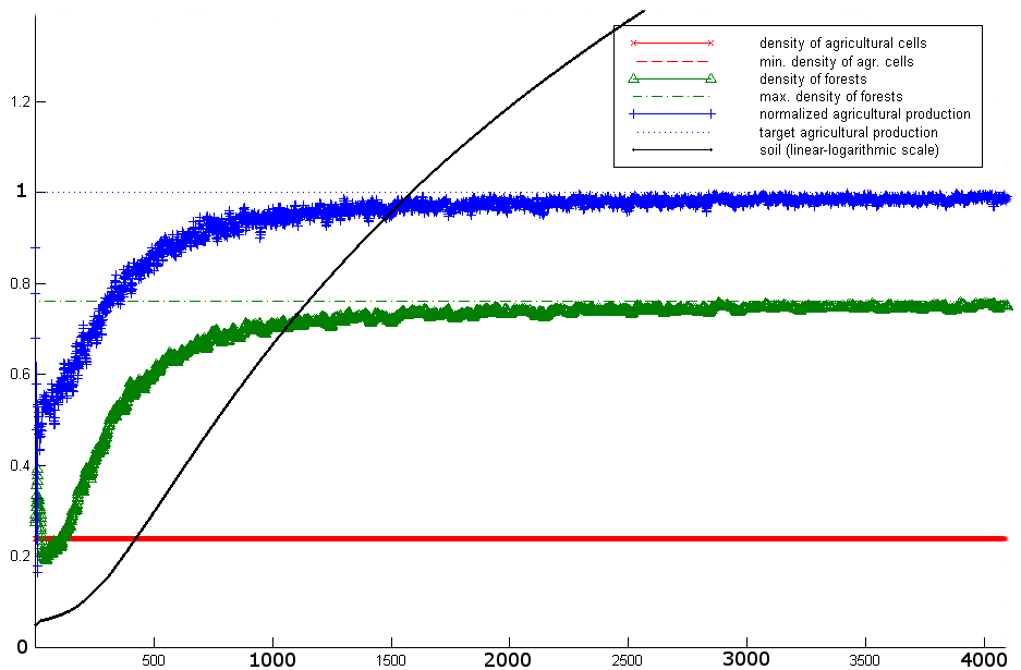
Figure 2: Illustration of long-term behaviour:
Sample simulation runs as in fig. 1 (strategy $\text{[S1]}_{\text{rand}}^{\text{(fix)}}$, parameters from tab. 2), except of the total simulation length $N_{t}=4096$. Run performed with (a) $\gamma_{\rm agr}=0.24$, (b) $\gamma_{\rm agr}=0.25$. See fig. 1 for a more detailed explanation of the quantities displayed in the plot.

Performing a larger number of runs for different sets of parameters shows that these are the two main outcomes of model runs: Either a positive level of forests is maintained and the agricultural production stabilizes at or close to the target production or forests vanish due to over-exploitation and the agricultural production breaks down to stabilize at a very low level, in particular significantly below the target production level.

3.2 Estimating Finite-Size Effects

The simulations shown in figs 1 to 2 have been performed on a $[32\times 32]$-grid. One can expect such simulations to be significantly affected by finite-size effects. In order to have at least a qualitative estimate for the severity of these effects, in fig. 3 we show the results for two simulations with parameters chosen as in fig. 1.a except that one has been performed on a $[16\times 16]$-, the other one on a $[64\times 64]$-grid.

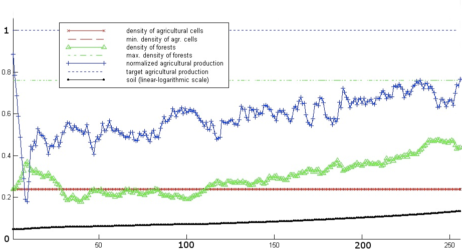
Figure 3: Estimate of finite-size effects: Sample simulation runs as in fig. 1 (strategy $\text{[S1]}_{\text{rand}}^{\text{(fix)}}$, parameters from tab. 2), with $\gamma_{\rm agr}=0.24$, except
(a) $N_{1}=N_{2}=16$, (b) $N_{1}=N_{2}=64$.
See fig. 1 for a more detailed explanation of the quantities displayed in the plot.

While for smaller grids the fluctuations (mostly induced by the stochastic nature of the model) are more pronounced, the general behaviour of the model seems to be quite insensitive to the size of the grid.

3.3 Dependence on Target Production Rate

While single simulation runs as depicted in figs. 1 to 3 give some hints on the characteristics of the model, a more systematic analysis is required for deeper insight. Therefore we have defined production target values

$$\gamma_{\rm agr}\in 0.01\cdot\{1,\,2,\,\ldots,\,34\}$$

and for each value performed 20 simulations with strategy $\text{[S1]}_{\text{rand}}^{\text{(fix)}}$ and parameters given in tab. 2.

The maximum value $\gamma_{\rm agr}=0.34$ has been chosen because the maximum sustainable normalized agricultural production $\gamma_{\rm max}$, determined by the linear equation

$$(1-\gamma_{\rm max})\,\max\left\{s^{(+)}_{(\text{pio})},\,s^{(+)}_{(\text{for})}\right\}-\gamma_{\rm max}\,s^{(-)}_{(\text{agr})}=1,$$ (12)

is equal to $\frac{1}{3}$ for the parameter values employed in the simulation.

In order to obtain a small number of characteristic numbers for each simulation run, we have recorded the density of agricultural cells, the density of forests, the normalized agricultural production and the amount of soil for the last $\frac{N_{t}}{4}=64$ timesteps, assuming that after $\frac{3N_{t}}{4}=192$ steps in most cases a characteristic state has been reached.

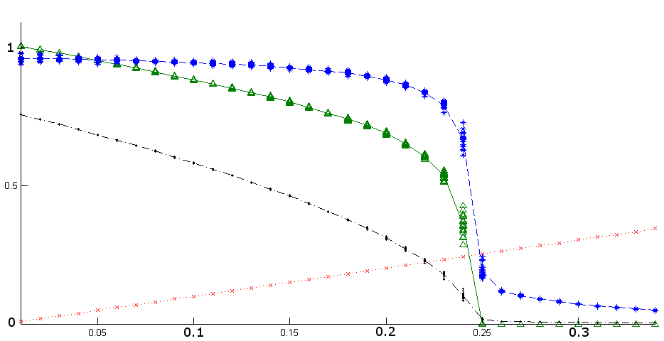
Figure 4: Typical structure of an overview plot: Summary of simulation runs for strategy $\text{[S1]}_{\text{rand}}^{\text{(fix)}}$ and standard parameters given in tab. 2. For each value of $\gamma_{\rm agr}\in 0.01\cdot\{1,\,2,\,\ldots,\,34\}$, 20 single simulations have been performed and the the values of characteristic quantities, averaged over the last 64 timesteps have been recorded. We show both the average for all 20 runs and the single results (in order to give an impression of the characteristic deviations). We plot the following quantities as function of the the target production rate $\gamma_{\rm agr}$:

	density of agricultural cells for the single runs,
	density of forest cells for the single runs,
	normalized agricultural production for the single runs,
	soil content (lin.-log. plot) for the single runs,
	density of agricultural cells, average value of all runs,
	density of forest cells, average value of all runs,
	normalized agricultural production, average value of all runs,
	soil content (lin.-log. plot), average value of all runs

The plot of results is shown in fig. 4. The dramatic transition between $\gamma_{\rm agr}=0.24$ and $\gamma_{\rm agr}=0.25$, already to be expected from a comparison of figs. 1.a and 1.b, is clearly visible here. The breakdown of agricultural production is accompanied by a steep drop of the density of forests. Only in the region $0.23\leq\gamma_{\rm agr}\leq 0.25$ there is a significant spread of the single results, which will is examined in more detail and discussed in sec. 3.4.

3.4 Analysis of the Transition Region

The overview plot shown in fig. 4 and discussed in sec. 3.3 clearly shows that for strategy $\text{[S1]}_{\text{rand}}^{\text{(fix)}}$ one has a significant spread of results only in a narrow transition region $0.23\leq\gamma_{\rm agr}\leq 0.25$.

This region has been analyzed in more detail. The corresponding overview plot and some histograms are displayed in figure 5. In particular for the target values $\gamma_{\rm agr}=0.2425$ and $\gamma_{\rm agr}=0.245$ the spread of production rates is large.

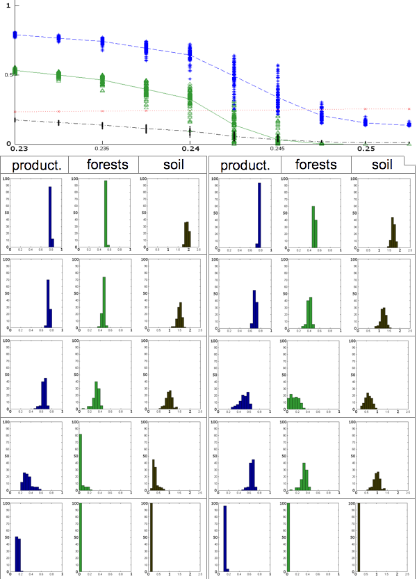
Figure 5: Detailed analysis of the transition region, performed for strategy $\text{[S1]}_{\text{rand}}^{\text{(fix)}}$. This figure contains an overview plot, structured as the one in fig. 4, but with 100 runs per single value of $\gamma_{\rm agr}\in\{0.23,\,0.2325,\,\ldots,\,0.25,\,0.2525\}$. In addition, for these values we show histogram plots, analogous to those presented in fig. 6. These are plots with 20 bins in $[0,\,1]$ or normalized production rate and for forest density, histogram plots with 25 bins in $[0,\,2.5]$ for the average amount of soil.

Two effects contribute to this spread: Both the basic update rules and (in this case) the strategy for the selection of new agricultural cells contain random elements. While these stochastic aspect seems to be of little importance for regions of clear success (here $\gamma_{\rm agr}<0.23$) and regions of clear failure (here $\gamma_{\rm agr}>0.25$), random events or choices may strongly influence the system in the critical region.

In addition, it is likely (though presumably very difficult to prove) that – beyond the influence of stochastic events – the update rules also contain aspects of chaotic behaviour. In particular the neighbourhood-dependent update rule for forests described by (2) may lead to situations where survival of the forest critically depends not only on the density, but also on the precise distribution of forest cells. In such cases, the initial configuration (which is also generated using random numbers) can be of crucial importance for the outcome.

In order to obtain a rough estimate of the importance of this effect, we have performed multiple simulation runs for the same initial configuration. The results (histograms for 100 runs with $\gamma_{\rm agr}=0.2425$ per initial configuration) for four distinct initial conditions are shown in fig. 6.

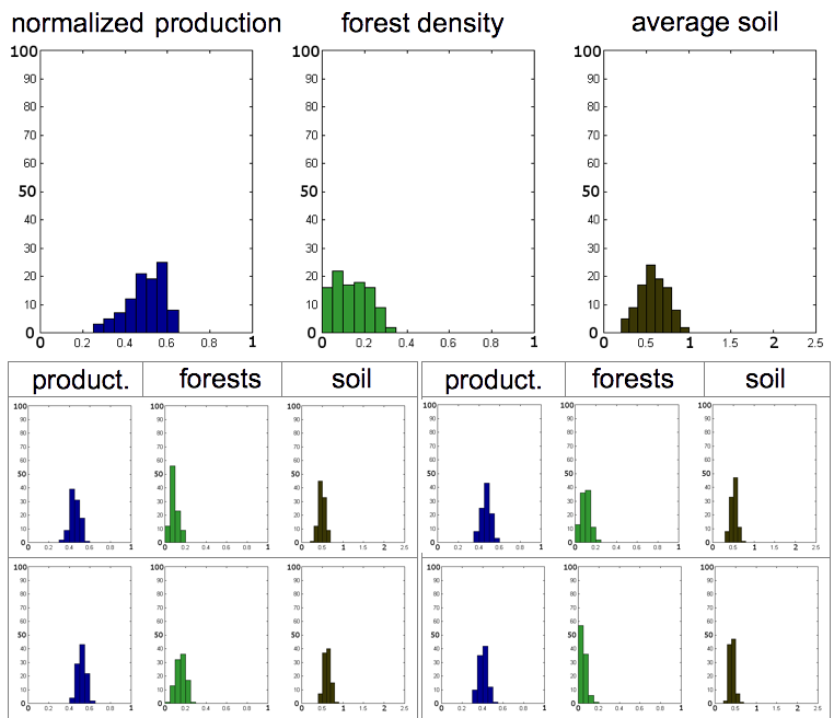
Figure 6: Influence of initial conditions, performed for strategy $\text{[S1]}_{\text{rand}}^{\text{(fix)}}$.
(a) Histogram for hundred different simulation runs for $\gamma_{\rm agr}=0.2425$ (the same histogram as the one already shown in fig. 5 for this value of $\gamma_{\rm agr}$, but enlarged).
(b) Histograms for four sets of simulation runs for $\gamma_{\rm agr}=0.2425$ with hundred runs per set, but this time for each distinct set only one (randomly chosen) initial configuration has been used. For each set, the spread of results can only be attributed to the dynamics of the system, not to sensitivity to initial conditions.
As in fig. 5, the histograms contain $20$ bins each, uniformly placed in the interval $[0,\,1]$ for normalized production rate and for forest density, $25$ bins uniformly placed in $[0,\,2.5]$ for the average amount of soil.

While the spread for runs with the same initial configuration is significantly smaller than for runs with different configurations, it is still present. This is at least some evidence (though by far no proof) that both random fluctuations and chaotic behaviour contribute to the spread of results in the transition region.

3.5 Robustness of the Model

All simulations so far have been performed with one set of parameters, given in tab. 2. For the model to be relevant, the qualitative behaviour should not depend heavily on the actual choice of parameters, as long as, for example, the ordering $s^{(+)}_{(\text{pio})}<s^{(+)}_{(\text{for})}<s^{(-)}_{(\text{agr})}$ is respected.

In order to check this for at least a few cases, in addition to tab. 2 we have defined two other sets of parameters, given in tab. 3 and created systematic plots similar to the one shown in fig. 4.

grid size & timesteps	$N_{1}=32$,	$N_{2}=32$,	$N_{t}=256$,
first modified set:	$\rho_{\text{for}}^{\text{(ini)}}=0.25$,	$\rho_{\text{pio}}^{\text{(ini)}}=0.25$,
	$p_{\text{pio}}=0.25$,	$\tau_{\text{for}}=0.75$,	$\tau_{\rm agri}=1$,
	$s^{(+)}_{(\text{pio})}=0.02$,	$s^{(+)}_{(\text{for})}=0.04$,	$s^{(-)}_{(\text{agr})}=0.12$
second modified set:	$\rho_{\text{for}}^{\text{(ini)}}=0.75$,	$\rho_{\text{pio}}^{\text{(ini)}}=0.75$,
	$p_{\text{pio}}=0.75$,	$\tau_{\text{for}}=0.25$,	$\tau_{\rm agri}=1$,
	$s^{(+)}_{(\text{pio})}=0.04$,	$s^{(+)}_{(\text{for})}=0.06$,	$s^{(-)}_{(\text{agr})}=0.08$

Table 3: Set of modified parameters, used for the simulations presented in sec. 3.5 and fig. 7.

The plots for the two alternative sets of parameters is shown in fig. 7. While the transitions from success ($A\approx A^{(\rm goal)}$) to failure ($A\ll A^{(\rm goal)}$) set in at different values of $\gamma_{\rm agr}$, the qualitative behaviour is essentially unaltered. This indicates that the model is robust with respect to variations of parameters.

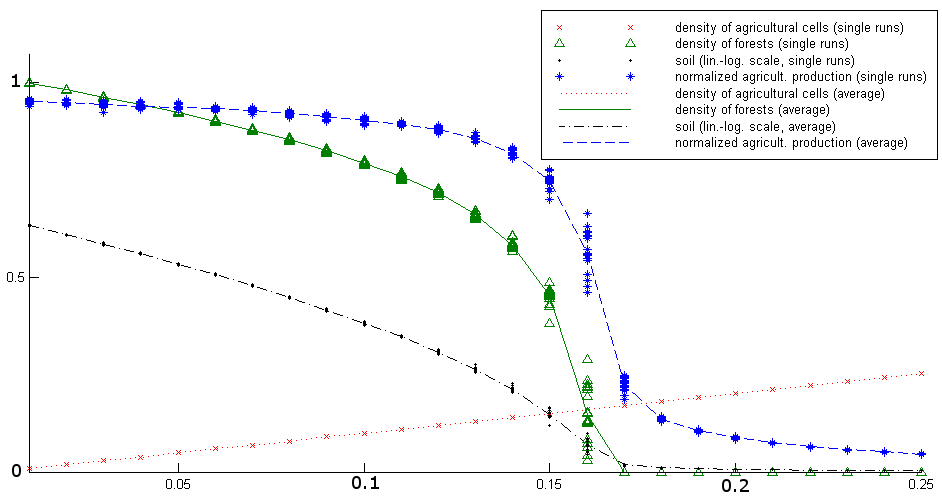
Figure 7: Overview plots for modified parameters: Simulation runs as in fig. 4 (strategy $\text{[S1]}_{\text{rand}}^{\text{(fix)}}$, 20 runs for each single value of $\gamma_{\rm agr}$), but with parameters taken from tab. 3 and performed for a different range for $\gamma_{\rm agr}$:
(a) Results for first modified set of parameters, $\gamma_{\rm agr}\in 0.01\cdot\{1,\,2,\,\ldots,\,25\}$,
(b) Results for second modified set of parameters, $\gamma_{\rm agr}\in 0.01\cdot\{1,\,2,\,\ldots,\,43\}$ See fig. 4 for a more detailed explanation of the quantities displayed in the plot.

4 Comparison of Strategies

All simulations in the sec. 3 have been performed with strategy $\text{[S1]}_{\text{rand}}^{\text{(fix)}}$. We now turn to some other management strategies outlined in sec. 2.2.4. The results for these simulations are shown as a combination of a comprehensive overview plot (such as the one shown in fig. 4) and two or three single runs (similar to the one shown in fig. 1), combined into one single figure.

4.1 Variable Number of Agricultural Fields

When employing strategy $\text{[S1]}_{\text{rand}}^{\text{(var)}}$, regarding the number of agricultural fields as variable, the transition between success and failure becomes even more pronounced than for strategy $\text{[S1]}_{\text{rand}}^{\text{(fix)}}$. For the standard choice of parameters, the system exhibits dramatic breakdown between $\gamma_{\rm agr}=0.16$ and $\gamma_{\rm agr}=0.17$, see fig. 8.

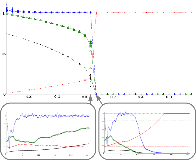
Figure 8: Overview plot for strategy $\text{[S1]}_{\text{rand}}^{\text{(var)}}$ with thumbnails of typical single runs for $\gamma_{\rm agr}=0.16$ and $\gamma_{\rm agr}=0.17$ included. The overview plot is structured the same way as the one in fig. 4, the single runs as the ones in fig. 1.

This type of behaviour can easily be explained. For small values of $\gamma_{\rm agr}$, the target production is easily reached and the degree of freedom provided by a variable number of fields is not used. For larger values of $\gamma_{\rm agr}$, when the production drops below the target, additional fields are created.

In the present case, for $\gamma_{\rm agr}\leq 0.16$, these additional fields make up for the production losses, and full productivity can be provided. For $\gamma_{\rm agr}\geq 0.17$, the increased number of fields reduces the number of cells available for regeneration of soil, which leads to a further increase of the number of fields – a positive feedback loop which leads to breakdown of the whole system and zero productivity.

In general, this type of behaviour can also be expected for other strategies with a variable number of fields. The transition will be more pronounced and failure will occur already at lower values of $\gamma_{\rm agr}$ than for the otherwise equivalent strategy with a fixed number of fields.

4.2 Optimized Choice of New Agricultural Fields

In strategy $\text{[S1]}_{\text{opt}}^{\text{(fix)}}$, the number of fields is kept fixed, but instead of beeing chosen randomly, new fields are chosen in an optimized way. This means that those cells with maximum amount of soil are converted to fields.

The results are shown in fig. 9. For $\gamma_{\rm agr}<0.25$, strategy works well, though there are some variations in productivity, as discussed below. The transition at $\gamma_{\rm agr}=0.25$ is sharp, but for this value one has a large spread of possible outcomes. While most simulation runs for this target fail, some are reasonable successful with a normalized productivy in the range of $80\%$ to $90\%$.

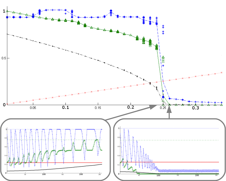
Figure 9: Overview plot for strategy $\text{[S1]}_{\text{opt}}^{\text{(fix)}}$ with thumbnails of typical single runs for $\gamma_{\rm agr}=0.24$ and $\gamma_{\rm agr}=0.26$ included. The overview plot is structured the same way as the one in fig. 4, the single runs as the ones in fig. 1.

For this strategy, a close look at single runs is particularly rewarding. Both in fig. 9.b and 9.c one has significant oscillations of productivity. While the first few periods are quite similar in both cases, soon the difference becomes clearly visible. For fig. 9.c, the height of the peaks drops and the average amount of forest during a cycle decreases. For fig. 9.b, the duration of maximum productivity during a single cycle increases (i.e. plateaus form).

However, steep drops in productivity occur also after considerable simulation time and while these drops seem to become less severe during the course of simulation, this happens only at a very slow pace.

These oscillations are, to a lesser extent, still present also for smaller values of $\gamma_{\rm agr}$. This is visible in fig. 9.a: Depending on whether or not such a characteristic drop in productivity is included in the averaging region (i.e. the last $64$ timesteps), the averaged production is either very close to the target or about $5\%$ below.

4.3 Optimized Choice with Variable Number of Fields

Strategy $\text{[S1]}_{\text{opt}}^{\text{(var)}}$ combines the modifications of secs. 4.1 and 4.2, i.e. new fields are chosen according to maximum soil and the number of fields is variable. Results are shown in fig. 10, and as already stated in sec. 4.1, a variable number of fields leads to a sharp transition and an earlier onset of failure. This strategy permits “over-shooting” the production goal, and for small values of $\gamma_{\rm agr}$, the normalized productivity tends to significantly exceed one.

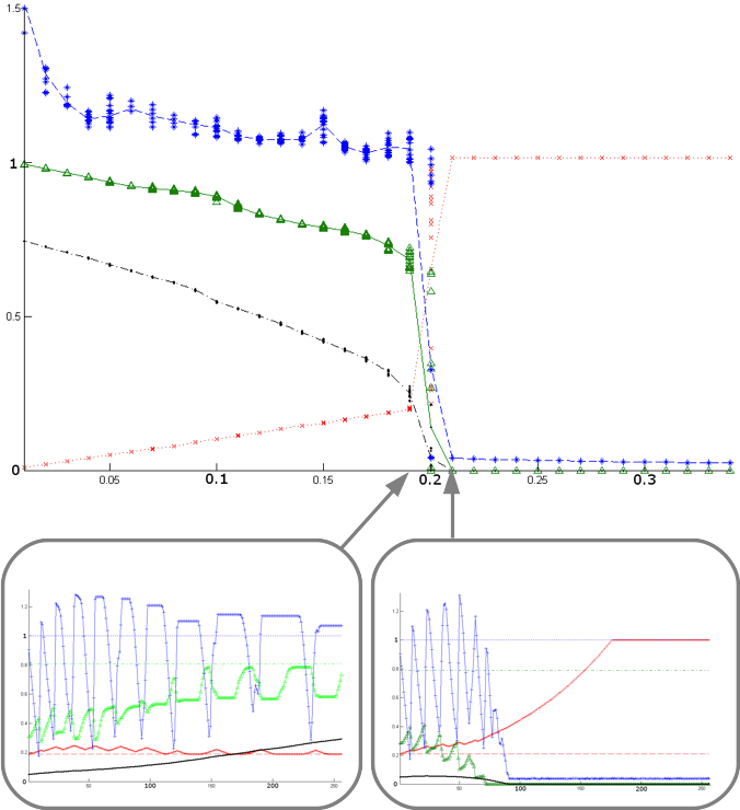
Figure 10: Overview plot for strategy $\text{[S1]}_{\text{opt}}^{\text{(var)}}$ with thumbnails of typical single runs for $\gamma_{\rm agr}=0.19$ and $\gamma_{\rm agr}=0.21$ included. The overview plot is structured the same way as the one in fig. 4, the single runs as the ones in fig. 1.

As it had already been the case in sec. 4.2, the single runs displayed as thumbnails in figs. 10 exhibit prominent cycles both in the case of success and of failure. In both cases a typical cycle includes a phase of over-production and a steep drop to $30\%$ productivity or less.

The difference between the two cases is not obvious during the first few cycles when just focussing on productivity. Also the number of fields and the amount of soil show strikingly similar behaviour. The best early indicator for success or failure seems to be the net increase or decrease of forest during a single cycle.

4.4 Abandoning Fields Below Threshold

An alternative to keeping fields as long as possible is to abandon fields already if the amount of soil drops below threshold. This is implemented in the different variations of stategy [S2]. One can expect that this strategy can avoid drops in productivity better than strategy [S1], as long as sufficient resources (i.e. cells with a sufficient amount of soil) are available.

As an example for this type of strategies, we have examined strategy $\text{[S2]}_{\text{rand}}^{\text{(fix)}}$; the results are displayed in fig. 11. As compared to the results for the otherwise equivalent strategy $\text{[S1]}_{\text{rand}}^{\text{(fix)}}$, displayed in fig. 4, on has a more stable production rate for $\gamma_{\rm agr}\leq 0.18$, but a sharp transition (with a wide spread of possible outcomes for the same target productivity) at $\gamma_{\rm agr}=0.19$.

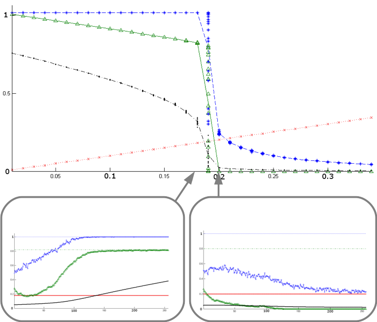
Figure 11: Overview plot for strategy $\text{[S2]}_{\text{rand}}^{\text{(fix)}}$ with thumbnails of typical single runs for $\gamma_{\rm agr}=0.18$ and $\gamma_{\rm agr}=0.20$ included. The overview plot is structured the same way as the one in fig. 4, the single runs as the ones in fig. 1.

As it has already been the case with strategies $\text{[S1]}_{\text{opt}}^{\text{(fix)}}$, a seemingly “smarter” strategy (corresponding to more efficient exploitation) leads to a sharper transition and an earlier breakdown of the system.

4.5 Redistribution of Fields

Strategy $\text{[S3]}_{\text{rand}}^{\text{(fix)}}$ includes random redistribution of fields at each timestep. The results are illustrated in fig. 12. Compared to the otherwise equivalent strategies $\text{[S1]}_{\text{rand}}^{\text{(fix)}}$ and $\text{[S2]}_{\text{rand}}^{\text{(fix)}}$, one has a smoother transition between high and low productivity.

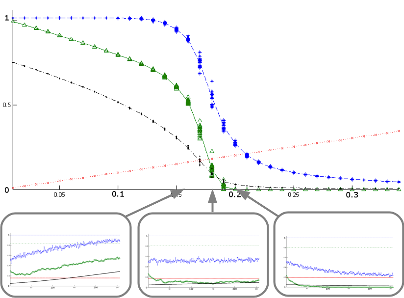
Figure 12: Overview plot for strategy $\text{[S3]}_{\text{rand}}^{\text{(fix)}}$ with thumbnails of typical single runs for $\gamma_{\rm agr}=0.16$, $\gamma_{\rm agr}=0.18$ and $\gamma_{\rm agr}=0.20$ included. The overview plot is structured the same way as the one in fig. 4, the single runs as the ones in fig. 1.

The normalized production has dropped to about $50\%$ at $\gamma_{\rm agr}\approx 0.18$, which is similar to the transition value found for $\text{[S2]}_{\text{rand}}^{\text{(fix)}}$ (see fig. 11) and significantly lower than the one found for $\text{[S1]}_{\text{rand}}^{\text{(fix)}}$ (see fig. 4).

4.6 Redistribution of Fields with Reforestation

In strategy $\text{[S4]}_{\text{rand}}^{\text{(fix)}}$, redistribution of fields is supplemented by reforestation, if possible; results are shown in fig. 13. The transition is even less dramatic than the one illustrated in fig. 12, and one still has reasonable productivity at high values of $\gamma_{\rm agr}$. The predefined production goal, however, can only be fulfilled for $\gamma_{\rm agr}\leq 0.15$, and it is clear from the graph that total productivity is maximum for an intermediate value of $\gamma_{\rm agr}$ and drops by further increasing the target production.

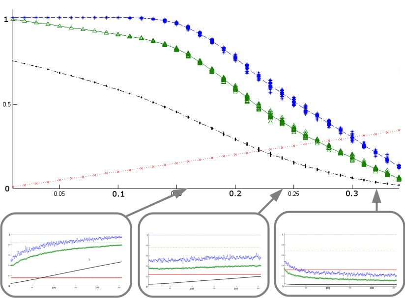
Figure 13: Overview plot for strategy $\text{[S4]}_{\text{rand}}^{\text{(fix)}}$ with thumbnails of typical single runs for $\gamma_{\rm agr}=0.16$, $\gamma_{\rm agr}=0.24$ and $\gamma_{\rm agr}=0.32$ included. The overview plot is structured the same way as the one in fig. 4, the single runs as the ones in fig. 1.

5 Discussion and Interpretation

The model described in sec. 2 and examined in secs. 3 and 4, while being quite simple, exhibits extremely interesting behaviour. In particular, for some strategies, as the ones labeled as [S1] and [S2] in sec. 2.2.4, one can have dramatic drops in productivity when just slightly raising the productivity goal above a critical value. A strategy that works very well with a specific target productivit can yield extremely poor results with a higher one.

A particularly interesting strategy is $\text{[S1]}_{\text{opt}}^{\text{(var)}}$, discussed in sec. 4.3. It is to some extent “intelligent” for choosing new fields in an optimized way and “flexible” for expanding the number of fields, if necessary. It is also “stubborn” since it does not give up fields even if productivity drops and “short-sighted” for not having a built-in sustainability strategy (in contrast to strategy [S4]) and putting no upper limit on the number of fields.

The properties of being “intelligent”, “flexible”, “stubborn” and “short-sighted” at the same time makes this strategy an excellent candidate model for typical human behaviour. Indeed, the patterns displayed in figs. 10.b and 10.c qualitatively resemble upturn and downturn cycles, most prominently known from economy. These cycles either leading to stabilization on a high level or to breakdown of the system.

Other strategies, as the ones labeled as [S3] and [S4] in sec. 2.2.4, are more stable in the sense that transitions are not so dramatic (though the domain of acceptable productivity does not need to be larger). Employing these strategies (re-distributing fields, possibly even with reforestation) means larger effort. In a more detailed approach, this effort could be taken into account by additional costs which reduce the net productivity.

While the model presented in sec. 2 has been formulated in terms of soil, forests and agricultural fields, it might serve as a quite general model for use and overuse of renewable resources. It might even be possible, to re-interpret it in other fields, as in psychological context. A simple model for burnout could be obtained with the substitution:

soil	$\to$	personal resources
pioneer plants	$\to$	recreational time
forest	$\to$	social activities
fields	$\to$	working hours
production goal	$\to$	prescribed workload

An alternative re-interpretation could be done for exampe in economic context, for example with the substitution:

soil	$\to$	existing infrastructure
pioneer plants	$\to$	private initiatives
forest	$\to$	community-based activities
fields	$\to$	exploitation of infrastructure
production goal	$\to$	expected profit

6 Summary and Outlook

We have presented an extended stochastic cellular automata model for the management of renewable resources, formulated in terms of soil, vegetation and agriculture (sec. 2), but general enough to be interpreted in various other ways (sec. 5).

On small grids the typical behaviour becomes clear already after a few hundred simulation steps (sec. 3.1), and the model seems to be robust with respect to finite size effects (sec. 3.2). Within a wide range, a change of parameters only leads to quantitative, but not to qualitative changes (sec. 3.5) of the results.

The behaviour of the model is strongly influenced by the management strategy employed (sec. 2.2.4). Simple strategies typically lead to sharp transitions between fulfillment of goals and a breakdown of the system (sec. 3 and secs. 4.1 to 4.4), possibly with several cycles before one or the other stable state is reached.

From these results one can conclude that a strategy which works very well for a specific target productivity may yield extremely poor results with respect to a higher one. Close to the critical value, raising the productivity even slightly higher can lead to desaster.

We also see that if more sophisticated strategies are chosen (secs. 4.5 and 4.6), less dramatic transitions occur. We note, however, that applying such strategies requires a larger effort. This could be taken into account by considering additional costs which reduce the net productivity.

The model offers many possibilities for further studies and for extensions. The strategies presented in sec. 2.2.4 and investigated in sec. 4 are far from being exhaustive, and it might be worthwile to examine more elaborate management strategies, in particular with a variable but limited number of agricultural cells.

Possible extensions that could be implemented include nature protection areas and elements of economy. For the latter one can take into account food price, but also the energy sector, since agriculture can act both as a source and as a sink of energy available to society.

Finally, one could include this model in a “small-world” climate model as the the one described in [8], in which plant growth and large-scale forest fires have significant influence on climate dynamics, while carbon dioxide concentration and temperature limit plant growth rates. Employing the present model would allow to include the carbon storage capacity of soil and impose an additional soil-quality constraint on plant growth rates.

References

- [1] D. H. Meadows, G. Meadows, J. Randers, W. W. Behrens III.: The Limits to Growth: a report for the Club of Rome’s project on the predicament of mankind, Universe Books, New York, 1972
- [2] D. H. Meadows, D. L. Meadows, J. Randers: Limits to Growth: The 30-Year Update, Chelsea Green Publishing, 2004
- [3] D. R. Montgomery: Dirt: The Erosion of Civilizations, University of California Press, 2007
- [4] Biodiversity At Risk Underfoot (Jim Robbins News Analysis, Helena, Montana), The New York Times International Weekly, May 17, 2013
- [5] P. Loveland, J. Webb, Soil & Tillage Research 70 (2003) 1-18, Is there a critical level of organic matter in the agricultural soils of temperate regions: a review
- [6] B. M. Petersen, J. Berntsen, S. Hansen, L. S. Jensen, Soil Biology & Biochemistry 37 (2005) 359-374, CN-SIM – a model for the turnover of soil organic matter. I. Long-term carbon and radiocarbon development
- [7] B. M. Petersen, L. S. Jensen, S. Hansen, A.Pedersen, T. M. Henriksen, P. Sørensen, I. Trinsoutrot-Gattin, J. Berntsen Soil Biology & Biochemistry 37 (2005) 375-393 CN-SIM: a model for the turnover of soil organic matter. II. Short-term carbon and nitrogen development
- [8] Klaus Lichtenegger, Wilhelm Schappacher, A Carbon-Cycle Based Stochastic Cellular Automata Climate Model, IJMPC 22, 6 (2011) pp. 607-621
- [9] Von Neumann J. et Burks A. ed., Theory of Self-Reproduction Automata, University of Illinois Press, 1966, p. 77, in Ostolaza J.L., Bergareche A.M., La vie artificielle, Seuil, Paris, 1997, pp. 37-38. Translated from French.
- [10] Klaus Lichtenegger, Stochastic Cellular Automata Models in Disease Spreading and Ecology, diploma thesis, 2005; available on http://physik.uni-graz.at/kll/cthesis.pdf
- [11] Klaus Lichtenegger, Wilhelm Schappacher, Phase Transition in a Stochastic Forest Fire Model and Effects of the Definition of Neighbourhood, IJMPC 20, 8 (2009) pp. 1247-1269