OFDM Synthetic Aperture Radar Imaging with Sufficient Cyclic Prefix

Abstract

The existing linear frequency modulated (LFM) (or step frequency) and random noise synthetic aperture radar (SAR) systems may correspond to the frequency hopping (FH) and direct sequence (DS) spread spectrum systems in the past second and third generation wireless communications. Similar to the current and future wireless communications generations, in this paper, we propose OFDM SAR imaging, where a sufficient cyclic prefix (CP) is added to each OFDM pulse. The sufficient CP insertion converts an inter-symbol interference (ISI) channel from multipaths into multiple ISI-free subchannels as the key in a wireless communications system, and analogously, it provides an inter-range-cell interference (IRCI) free (high range resolution) SAR image in a SAR system. The sufficient CP insertion along with our newly proposed SAR imaging algorithm particularly for the OFDM signals also differentiates this paper from all the existing studies in the literature on OFDM radar signal processing. Simulation results are presented to illustrate the high range resolution performance of our proposed CP based OFDM SAR imaging algorithm.

I Introduction

Synthetic aperture radar (SAR) can perform well to image under almost all weather conditions [1], which, in the past decades, has received considerable attention. Several types of SAR systems using different transmitted signals have been well developed and analyzed, such as the linear frequency modulated (LFM) chirp radar [2], linear/random step frequency radar [1, 3], and random noise radar [4, 5, 6].

Recently, orthogonal frequency-division multiplexing (OFDM) signals have been used in radar applications, which may provide opportunities to achieve ultrawideband (UWB) radar. OFDM radar signal processing was first presented in [7] and was also studied in [8, 9, 10, 11, 12, 13]. Adaptive OFDM radar was investigated for moving target detection and low-grazing angle target tracking in [14, 15, 16]. Using OFDM signals for SAR applications was proposed in [17, 18, 19, 20, 21, 22, 23]. In [17, 18, 19], adaptive OFDM signal design was studied for range ambiguity suppression in SAR imaging. The reconstruction of the cross-range profiles is studied in [22, 23]. Signal processing of a passive OFDM radar using digital audio broadcast (DAB), digital video broadcast (DVB), Wireless Fidelity (WiFi) or worldwide inoperability for microwave access (WiMAX) signals for target detection and SAR imaging was investigated in [24, 25, 26, 27, 28, 29, 30]. However, all the existing OFDM radar (including SAR) signal processing is on radar waveform designs with ambiguity function analyses to mitigate the interferences between range/cross-range cells using multicarrier signals similar to the conventional waveform designs and the radar receivers, such as SAR imaging algorithms, are basically not changed. The most important feature of OFDM signals in communications systems, namely, converting an intersymbol-interference (ISI) channel to multiple ISI-free subchannels, when a sufficient cyclic prefix (CP) is inserted, has not been utilized so far in the literature. In this paper, we will fully take this feature of the OFDM signals into account to propose OFDM SAR imaging where a sufficient CP is added to each OFDM pulse, as the next generation high range resolution SAR imaging. In our proposed SAR imaging algorithm, not only the transmission side but also the receive side are different from the existing SAR imaging methods. To further explain it, let us briefly overview some of the key signalings in SAR imaging.

To achieve long distance imaging, a pulse with long enough time duration is used to carry enough transmit energy [31]. The received pulses from different scatterers are overlapped with each other and cause energy interferences between these scatterers. To mitigate the impact of the energy interferences and achieve high resolution, the transmitted pulse is coded using frequency or phase modulation (i.e., LFM signal and step frequency signal) or random noise type signals in random noise radar to achieve a bandwidth $B$ which is large compared to that of an uncoded pulse with the same time duration [31]. This is similar to the spread spectrum technique in communications systems. Then, pulse compression techniques are applied at the receiver to yield a narrow compressed pulse response. Thus, the reflected energies from different range cells can be distinguished [31]. However, the energy interferences between different range cells, that we regard as inter-range-cell interference (IRCI), still exist because of the sidelobes of the ambiguity function of the transmitted signal, whose sidelobe magnitude is roughly $\sqrt{N}$ if the mainlobe of the modulated signal pulse is $N$ [32]. This IRCI is much significant in SAR imaging [2]. Despite of the IRCI, the existing well-known/used SAR are LFM (or step frequency) SAR [2, 3] and random noise SAR [4, 5, 6].

We are adopting the OFDM technique [33] that is the key technology in the latest wireless communications standards, such as long term evolution (LTE) [34] and WiFi. If we think about only one user in a wireless communications system, there are similarity and difference between wireless communications systems and SAR imaging systems. The similarity is that both systems are transmitting and receiving signals reflected from various scatterers and the numbers of multipaths depend on the transmitted signal bandwidths. The difference is that in communications systems, the receiver cares about the transmitted signal, while in SAR imaging systems, the receiver cares about the scatterers within different range cells (with different time delays) that reflect and cause multipath signals. The multipaths cause ISI in communications, while the multipaths cause the IRCI in SAR imaging systems. The higher the bandwidth is, the more multipaths there are in communications systems, and the more range cells there are for a fixed imaging scene (or swath width), i.e., the higher the range resolution is, in SAR imaging systems. The existing well-known/used LFM (or step frequency) and random noise SAR systems, in fact, correspond to the two spread spectrum systems, i.e., frequency hopping (FH) and direct sequence (DS) in CDMA systems [35], which work well in non-high bandwidth wireless communications systems, such as the second and the third generations of cellular communications, of less than $10$ MHz (roughly) bandwidth. They, however, may not work well for a system of a much higher signal bandwidth, such as $20$ MHz in LTE, due to the severe ISI caused by too many multipaths. In contrast, since OFDM with a sufficient CP can convert an ISI channel to multiple ISI-free subchannels, as mentioned earlier, it is used in the latest LTE and WiFi standards. As an analogy, one expects that LFM and random noise SAR may not work too well for high bandwidth radar systems where there are too many range cells in one cross range, which cause severe IRCI due to the significant sidelobes of the ambiguity functions of the LFM and random signals. On the other hand, in order to have a high range resolution, a high bandwidth is necessary. Therefore, borrowing from wireless communications, in this paper we propose to use OFDM signals with sufficient CP to deal with the IRCI problem as a next generation SAR imaging to produce a high range resolution SAR image. We show that, in our proposed OFDM SAR imaging with a sufficient CP, the sidelobes are ideally zero, and for any range cell, there will be no IRCI from other range cells in one cross range.

Another difference for OFDM communications systems and CP based OFDM SAR systems is as follows. It is known in communications that, for an OFDM system, a Doppler frequency shift is not desired, while the azimuth domain (or cross range direction) in a SAR imaging system is, however, generated from the relative Doppler frequency shifts between the radar platform and the scatterers. One might ask how the OFDM signals are used to form a SAR image. This question is not difficult to answer. The range distance between radar platform and image scene is known and the radar platform moving velocity is known too. Thus, the Doppler shifts are also known, which can be used to generate the cross ranges similar to other SAR imaging techniques, and can be also used to compensate the Doppler shift inside one cross range and correct the range migration.

This paper is organized as follows. In Section II, we propose our CP based OFDM SAR imaging algorithm. In Section III, we present some simulations to illustrate the high range resolution property of the proposed CP based OFDM SAR imaging and also the necessity of a sufficient CP insertion in an OFDM signal. In Section IV, we conclude this paper and point out some future research problems.

II System Model and CP Based OFDM SAR Imaging

In this section, we first describe the OFDM SAR signal model, and then propose the corresponding SAR imaging algorithm.

II-A OFDM SAR signal model

In this paper, we consider the monostatic broadside stripmap SAR geometry as shown in Fig. 1. The radar platform is moving parallelly to the $y$-axis with an instantaneous coordinate $\left(0,y_{p}(\eta),H_{p}\right)$, $H_{p}$ is the altitude of the radar platform, $\eta$ is the relative azimuth time referenced to the time of zero Doppler, $T_{a}$ is the synthetic aperture time defined by the azimuth time extent the target stays in the antenna beam. For convenience, let us choose the azimuth time origin $\eta=0$ to be the zero Doppler sample. Consider an OFDM signal with $N$ subcarriers, a bandwidth of $B$ Hz, and let ${\mbox{\boldmath{$S$}}}=\left[S_{0},S_{1},\ldots,S_{N-1}\right]^{T}$ represent the complex weights transmitted over the subcarriers, and $\sum\limits_{k=0}^{N-1}\left|S_{k}\right|^{2}=N$. Then, a discrete time OFDM signal is the inverse fast Fourier transform (IFFT) of the vector $S$ and the OFDM pulse is

$$s\left(t\right)=\frac{1}{\sqrt{N}}\sum_{k=0}^{N-1}S_{k}\textrm{exp}\left\{j2\pi k\Delta ft\right\},\ t\in\left[0,T+T_{GI}\right],$$ (1)

where $\Delta f=\frac{B}{N}=\frac{1}{T}$ is the subcarrier spacing. $\left[0,T_{GI}\right)$ is the time duration of the guard interval that corresponds to the CP in the discrete time domain as we shall see later in more details and its length $T_{GI}$ will be specified later too, $T$ is the length of the OFDM signal excluding CP. Due to the periodicity of the exponential function $\textrm{exp}(\cdot)$ in (1), the tail part of $s\left(t\right)$ for $t$ in $\left(T,T+T_{GI}\right]$ is the same as the head part of $s\left(t\right)$ for $t$ in $\left[0,T_{GI}\right)$. Let $f_{c}$ be the carrier frequency of operation, the transmitted signal is given by

$$s_{1}\left(t\right)=\textrm{Re}\left\{\frac{1}{\sqrt{N}}\sum_{k=0}^{N-1}S_{k}\textrm{exp}\left\{j2\pi f_{k}t\right\}\right\},\ t\in\left[0,T+T_{GI}\right],$$ (2)

where $f_{k}=f_{c}+k\Delta f$ is the $k$th subcarrier frequency.

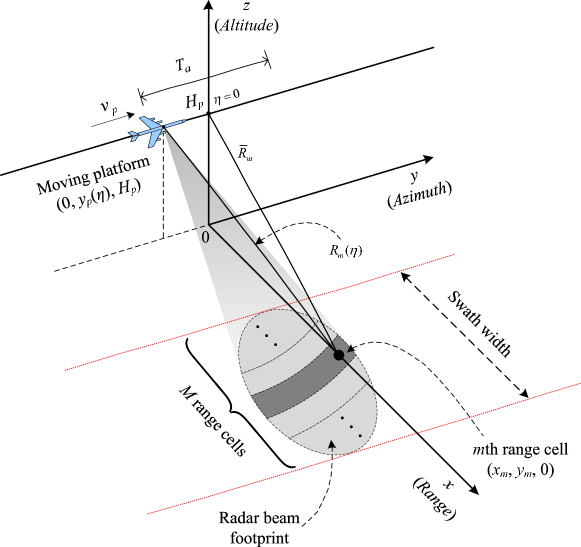
Figure 1: Monostatic stripmap SAR geometry.

After the demodulation to baseband, the complex envelope of the received signal from a static point target in the $m$th range cell can be written in terms of fast time $t$ and slow time $\eta$

$$\begin{array}[]{ll}u_{m}\left(t,\eta\right)&={g_{m}}\varepsilon_{a}(\eta)\textrm{exp}\left\{-j4\pi f_{c}\frac{R_{m}(\eta)}{c}\right\}\\ &\times\frac{1}{\sqrt{N}}\sum\limits_{k=0}^{N-1}S_{k}\textrm{exp}\left\{\frac{j2\pi k}{T}\left[t-\frac{2R_{m}(\eta)}{c}\right]\right\}+w(t,\eta),\ t\in\left[\frac{2R_{m}(\eta)}{c},\frac{2R_{m}(\eta)}{c}+T+T_{GI}\right],\\ \end{array}$$ (3)

where $\varepsilon_{a}(\eta)=p_{a}^{2}\left(\theta(\eta)\right)$ is the azimuth envelope, $p_{a}(\theta)\approx\textrm{sinc}\left(\frac{0.886\theta}{\beta_{bw}}\right)$ [2], $\textrm{sinc}(x)=\frac{\textrm{sin}(x)}{x}$ is the sinc function, $\theta$ is the angle measured from boresight in the slant range plane, $\beta_{bw}=\frac{0.866\lambda}{L_{a}}$ is the azimuth beamwidth, $L_{a}$ is the effective length of the antenna, $g_{m}$ is the radar cross section (RCS) coefficient caused from the scatterers in the $m$th range cell within the radar beam footprint, and $c$ is the speed of light. $w(t,\eta)$ represents the noise. $R_{m}(\eta)$ is the instantaneous slant range between the radar and the $m$th range cell with the coordinate $(x_{m},y_{m},0)$ and it can be written as

$$R_{m}(\eta)=\sqrt{\bar{R}_{m}^{2}+\left(y_{m}-y_{p}\left(\eta\right)\right)^{2}}=\sqrt{\bar{R}_{m}^{2}+v_{p}^{2}\eta^{2}},$$ (4)

where $\bar{R}_{m}=\sqrt{x_{m}^{2}+H_{p}^{2}}$ is the slant range when the radar platform and the target in the $m$th range cell are the closest approach, and $v_{p}$ is the effective velocity of the radar platform.

Figure 2: Illustration diagram of one range line.

Then, the complex envelope of the received signal from all the range cells in a swath can be written as

$$u(t,\eta)=\sum_{m}u_{m}(t,\eta).$$ (5)

At the receiver, with the A/D converter, the received signal is sampled with sampling interval $T_{s}=\frac{1}{B}$ and the range resolution is $\rho_{r}=\frac{c}{2B}$. Assume that the swath width for the radar is $R_{w}$. Let $M=\frac{R_{w}}{\rho_{r}}$ that is determined by the radar system. Then, a range profile can be divided into $M$ range cells as shown in Fig. 2. As we mentioned earlier, the main reason why OFDM has been successfully adopted in both recent wireline and wireless communications systems is its ability to deal with multipaths (they cause ISI in communications) that become more severe when the signal bandwidth is larger. In our radar applications here, the response of each range cell, formed by the summation of the responses of all scatterers within this range cell, contains its own delay and phase. Thus, to a transmitted pulse, each range cell can be regarded as one path of communications. $M$ range cells correspond to $M$ paths. Excluding one main path (i.e., the nearest range cell), there will be $M-1$ multipaths. To convert the ISI caused from the multipaths to the ISI free case in communications, a guard interval (or CP) needs to be added to each OFDM block and the CP length can not be smaller than the number of multipaths that is $M-1$ in this paper. Although in the radar application here, ISI is not the concern, the $M$ range cell paths are superposed (or interfered) together in the radar return signal, which is the same as the ISI in communications. So, in order to convert these interfered $M$ range cells to individual range cells without any IRCI, similar to OFDM systems in communications, the CP length should be at least $M-1$. For convenience, we use CP length $M-1$ in this paper, i.e., a CP of length $M-1$ is added at the beginning of an OFDM pulse, and then the guard interval length $T_{GI}$ in the analog transmission signal is $T_{GI}=(M-1)T_{s}$. Notice that $T=NT_{s}$, so the time duration of an OFDM pulse is $T_{o}=T+T_{GI}=(N+M-1)T_{s}$. In this paper, we assume $N\geq M$, i.e., the number of subcarriers of the OFDM signal is at least the number of range cells in a swath (or a cross range), which is similar to the application in communications [33, 35]. When $N<M$, the IRCI occurs and the detailed reason will be seen later.

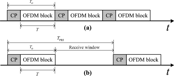
Figure 3: Transmission comparison of OFDM signals in (a) communications systems and (b) SAR systems.

In communications applications, to achieve a high transmission throughput, the OFDM pulses are transmitted consecutively as shown in Fig. 3(a). However, in SAR imaging applications, for monostatic case, the transmitter and receiver share the same antenna, which can not both transmit and receive signals at the same time and transmission throughput is not a concern. Thus, transmitted signals and radar return signals are usually separated in time. This implies that a reasonable receive window is needed between two consecutive pulses as shown in Fig. 3(b). For convenience, similar to what is commonly done in SAR systems, in this paper, we assume that the pulse repetition interval (PRI) is long enough so that all of the range cells in a swath fall within the receive window. Therefore, the PRI length $T_{\textrm{PRI}}$ should be

$$T_{\textrm{PRI}}=\frac{1}{\textrm{PRF}}>\left(\frac{2R_{w}}{c}+T_{o}\right),$$ (6)

where $R_{w}=M\rho_{r}$ is the swath width. We want to emphasize here that in our common SAR imaging applications, the pulse repetition frequency (PRF) may not be too high [2] and there is sufficient time duration to add a CP (a guard interval) for an OFDM pulse.

For Fig. 2, we notice that $R_{m}(\eta)=R_{0}(\eta)+m\rho_{r}$. Thus, $t-\frac{2R_{m}(\eta)}{c}$ in (3) can be written as

$$\begin{array}[]{ll}t-\frac{2R_{m}(\eta)}{c}&=t-\frac{2\left(R_{0}(\eta)+m\rho_{r}\right)}{c}\\ &=t-t_{0}(\eta)-mT_{s},\\ \end{array}$$ (7)

where for each $\eta$, the constant time delay $t_{0}(\eta)=\frac{2R_{0}(\eta)}{c}$ is independent of $m$. Let the sampling be aligned with the start of the received pulse after $t_{0}(\eta)$ seconds for the first arriving version of the transmitted pulse. Combining with (3), (7) and (5), $u(t,\eta)$ can be converted to the discrete time linear convolution of the transmitted sequence with the weighting RCS coefficients $d_{m}$, and the received sequence can be written as

$$u_{i}=\sum_{m=0}^{M-1}d_{m}s_{i-m}+w_{i},\ i=0,1,\ldots,N+2M-3,$$ (8)

where

$$d_{m}=g_{m}\varepsilon_{a}(\eta)\textrm{exp}\left\{-j4\pi f_{c}\frac{R_{m}(\eta)}{c}\right\},$$ (9)

in which $4\pi f_{c}\frac{R_{m}(\eta)}{c}$ in the exponential is the azimuth phase, and $s_{i}$ is the complex envelope of the OFDM pulse in (1) with time duration $t\in\left[0,T+T_{GI}\right]$ for $T=NT_{s}$ and $T_{GI}=(M-1)T_{s}$. After sampling at $t=iT_{s}$, (1) can be recast as:

$$s_{i}=s\left(iT_{s}\right)=\frac{1}{\sqrt{N}}\sum_{k=0}^{N-1}S_{k}\textrm{exp}\left\{\frac{j2\pi ki}{N}\right\},\ i=0,1,\ldots,N+M-2,$$ (10)

and $s_{i}=0$ if $i<0$ or $i>N+M-2$.

Notice that the transmitted sequence with CP is $\tilde{{\mbox{\boldmath{$s$}}}}=\left[s_{0},s_{1},\ldots,s_{N+M-2}\right]^{T}$, where $\left[s_{0},\ldots,s_{M-2}\right]^{T}=\left[s_{N},\ldots,s_{N+M-2}\right]^{T}$. The vector ${\mbox{\boldmath{$s$}}}=\left[s_{0},s_{1},\ldots,s_{N-1}\right]^{T}$ is indeed the IFFT of the vector ${\mbox{\boldmath{$S$}}}=\left[S_{0},S_{1},\ldots,S_{N-1}\right]^{T}$.

II-B Range compression

When the signal in (8) is received, the first and the last $M-1$ samples are removed, and then, we obtain

$$u_{n}=\sum_{m=0}^{M-1}d_{m}s_{n-m}+w_{n},\ n=M-1,M,\ldots,N+M-2.\\$$ (11)

Then, the received signal ${\mbox{\boldmath{$u$}}}=\left[u_{M-1},u_{M},\ldots,u_{N+M-2}\right]^{T}$ is

$$\begin{bmatrix}u_{M-1}\\ u_{M}\\ \vdots\\ u_{N+M-2}\end{bmatrix}=\begin{bmatrix}d_{M-1}&\cdots&d_{0}&\cdots&\cdots&0&\cdots&0\\ 0&d_{M-1}&\cdots&d_{0}&\cdots&0&\cdots&0\\ \vdots&\ddots&\ddots&\ddots&\ddots&\ddots&\ddots&\vdots\\ 0&\cdots&0&\cdots&\cdots&d_{M-1}&\cdots&d_{0}\end{bmatrix}\begin{bmatrix}s_{0}\\ \vdots\\ s_{M-1}\\ s_{M}\\ \vdots\\ s_{N+M-2}\end{bmatrix}+\begin{bmatrix}w_{M-1}\\ w_{M}\\ \vdots\\ w_{N+M-2}\end{bmatrix}.$$ (12)

Since $\left[s_{0},\ldots,s_{M-2}\right]^{T}=\left[s_{N},\ldots,s_{N+M-2}\right]^{T}$, it is not hard to see that the vector $\tilde{{\mbox{\boldmath{$s$}}}}=\left[s_{0},s_{1},\ldots,\right.$ $\!\!\!\left.s_{N+M-2}\right]^{T}$ in (12) can be replaced by its tail part ${\mbox{\boldmath{$s$}}}^{\prime}$, which can be also seen, in, for example, [35, Ch. 12.4], then, the matrix representation (12) is equivalent to the following representation:

$${\mbox{\boldmath{$u$}}}={\mbox{\boldmath{$H$}}}{\mbox{\boldmath{$s$}}}^{\prime}+{\mbox{\boldmath{$w$}}},$$ (13)

where ${\mbox{\boldmath{$s$}}}^{\prime}=\left[s_{M-1},s_{M},\cdots,s_{N+M-2}\right]^{T}=\left[s_{M-1},\cdots,s_{N-1},s_{0},\cdots,s_{M-2}\right]^{T}$, ${\mbox{\boldmath{$w$}}}=\left[w_{M-1},w_{M},\ldots,\right.$ $\!\!\!\left.w_{N+M-2}\right]^{T}$ and $H$ is built by superposing the first $M-1$ columns of the weighting RCS coefficient matrix in (12) to its last $M-1$ columns. And $H$ can be given by the following $N$ by $N$ matrix:

$${\mbox{\boldmath{$H$}}}=\begin{bmatrix}d_{0}&0&\cdots&0&d_{M-1}&\cdots&d_{1}\\ \vdots&\ddots&\ddots&\vdots&\ddots&\ddots&\vdots\\ d_{M-2}&\cdots&d_{0}&0&\cdots&0&d_{M-1}\\ d_{M-1}&d_{M-2}&\cdots&d_{0}&0&\cdots&0\\ 0&\ddots&\ddots&\vdots&\ddots&\ddots&\vdots\\ \vdots&\ddots&d_{M-1}&d_{M-2}&\cdots&d_{0}&0\\ 0&\cdots&0&d_{M-1}&d_{M-2}&\cdots&d_{0}\end{bmatrix}.$$ (14)

One can see that the matrix $H$ in (14) is a circulant matrix that can be diagonalized by the discrete Fourier transform (DFT) matrix of the same size.

The OFDM demodulator then performs a fast Fourier transform (FFT) on the vector $u$:

$$U_{k}=\frac{1}{\sqrt{N}}\sum_{n=0}^{N-1}u_{n+M-1}\textrm{exp}\left\{\frac{-j2\pi kn}{N}\right\},\ k=0,1,\ldots,N-1.$$ (15)

From (13)-(14), the above $U_{k}$ can be expressed as:

$$U_{k}=D_{k}S_{k}^{\prime}+W_{k},\ k=0,1,\ldots,N-1,$$ (16)

where $\left[S_{0}^{\prime},S_{1}^{\prime},\cdots,S_{N-1}^{\prime}\right]^{T}$ is the FFT of the vector ${\mbox{\boldmath{$s$}}}^{\prime}$, a cyclic shift of the vector $s$ of amount $M-1$, i.e., $S_{k}^{\prime}=S_{k}\textrm{exp}\left\{\frac{j2\pi k(M-1)}{N}\right\}$, $W_{k}$ is the FFT of the noise, and

$$D_{k}=\sum_{m=0}^{M-1}d_{m}\textrm{exp}\left\{\frac{-j2\pi mk}{N}\right\}.$$ (17)

Then, the estimate of $D_{k}$ is

$$\hat{D}_{k}=\frac{U_{k}}{S_{k}^{\prime}}=\frac{U_{k}}{S_{k}\textrm{exp}\left\{\frac{j2\pi k(M-1)}{N}\right\}}=D_{k}+\frac{W_{k}}{S_{k}}\textrm{exp}\left\{\frac{-j2\pi k(M-1)}{N}\right\},\ k=0,1,\ldots,N-1.$$ (18)

Notice that if $S_{k}$ is small, the noise is enhanced. Thus, for the constraint condition $\sum\limits_{k=0}^{N-1}\left|S_{k}\right|^{2}=N$, from (18) the optimal signal $S_{k}$ should have constant module for all $k$.

The vector ${\mbox{\boldmath{$D$}}}=\left[D_{0},D_{1},\ldots,D_{N-1}\right]^{T}$ is indeed the $N$-point FFT of $\sqrt{N}{\mbox{\boldmath{$\gamma$}}}$, where $\gamma$ is the weighting RCS coefficient vector:

$${\mbox{\boldmath{$\gamma$}}}=\left[d_{0},d_{1},\cdots,d_{M-1},\underbrace{0,\cdots,0}_{N-M}\right]^{T}.$$ (19)

So, the estimate of $d_{m}$ can be achieved by the $N$-point IFFT on the vector $\hat{{\mbox{\boldmath{$D$}}}}=\left[\hat{D}_{0},\hat{D}_{1},\ldots,\hat{D}_{N-1}\right]^{T}$:

$$\hat{d}_{m}=\frac{1}{\sqrt{N}}\sum_{k=0}^{N-1}\hat{D}_{k}\textrm{exp}\left\{\frac{j2\pi mk}{N}\right\},\ m=0,\ldots,M-1.\\$$ (20)

Then, we obtain the following estimates of the $M$ range cell weighting RCS coefficients:

$$\hat{d}_{m}={\sqrt{N}}d_{m}+\tilde{w}_{m}^{\prime},\ m=0,\ldots,M-1,$$ (21)

where $\tilde{w}_{m}^{\prime}$ is from the noise and its variance is the same as that in (18) since the IFFT implemented in (20) is a unitary transform. In $(\ref{estimated})$, $d_{m}$ can be completely recovered without any IRCI from other range cells. From (9), when $d_{m}$ are determined, the RCS coefficients $g_{m}$ are determined, and vice versa.

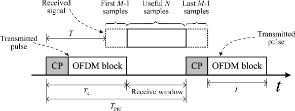
Figure 4: Transmitted and received timing of OFDM SAR system for $M=N$.

For $N>M$, there are some zeros in the vector $\gamma$ in (19). Considering (19) and (20), we notice that part of the transmitted OFDM sequence is used to estimate the unreal weighting RCS coefficients, i.e., the zeros in $\gamma$.

When $N=M$, there is no zeros included in the vector $\gamma$ in (19). We name this special case as swath width matched pulse (SWMP). The OFDM pulse length (excluding CP) $T=NT_{s}$ and the swath width $M\rho_{r}$ follow the relationship of $M\rho_{r}=\frac{cT}{2}$, i.e., the range resolution of a pulse with time duration $T$ is just the swath width $M\rho_{r}$ without range compression processing. And $\frac{cT}{2}$ is the maximal swath width that we can obtain without IRCI. Thus, the optimal time duration of the OFDM pulse is $T_{o}=(2N-1)T_{s}$ with CP length $N-1$, which is the maximal possible CP length for an OFDM sequence of length $N$.

Since the first and the last $M-1$ samples of the received sequence $u_{i}$ in (8) are removed, the receiver only needs to sample the received signal from $t=T_{0}$ to $t=T_{0}+T$, even when the radar return signal starts to arrive at time $t=T$ as shown in Fig. 4. Therefore, the minimum range of the OFDM radar is $\frac{cT}{2}$, the same as that of the traditional pulse radar of transmitted pulse length $T$. Notice that the minimum range is just the same as the maximal swath width. Thus, if we want to increase the swath width to, e.g., $10$ km, the transmitted pulse duration $T_{o}$ should be increased to about $133.3\ \mu s$ and the minimum range is increased to $10$ km. Also, the minimum receive window is just the OFDM pulse length $T$ (excluding CP) as Fig. 4, and the PRI length follows $T_{\textrm{PRI}}>T_{o}+T$. As a remark, different from the applications in communications where the CP is an overhead and may reduce the transmission data rate, in the SWMP case in SAR applications here, the longer the CP length is, the less the IRCI is, which leads to a better (high resolution) SAR image.

When $N<M$, according to (10) the signal vector $\left[s_{0},\cdots,s_{M-1},s_{M},\cdots,s_{N+M-2}\right]^{T}$ in (12) is $\left[s_{0},\ldots,s_{N-1},s_{0},\ldots,s_{N-1},\ldots,s_{(N+M-2)_{N}}\right]^{T}$, where $(n)_{N}$ is the residue of $n$ modulo $N$. Thus, the $N$ by $N$ matrix $H$ in (13) and (14) becomes

$${\mbox{\boldmath{$H$}}}=\begin{bmatrix}\tilde{d}_{0}&\tilde{d}_{N-1}&\cdots&\tilde{d}_{1}\\ \tilde{d}_{1}&\tilde{d}_{0}&\cdots&\tilde{d}_{2}\\ \vdots&\vdots&\ddots&\vdots\\ \tilde{d}_{N-1}&\tilde{d}_{N-2}&\cdots&\tilde{d}_{0}\end{bmatrix},$$ (22)

where $\tilde{d}_{n}=\sum\limits_{i:\ 0\leq iN+n\leq M-1}d_{iN+n},\ n=0,\ldots,N-1$. One can see, $\tilde{d}_{n}$ is a summation of weighting RCS coefficients from several range cells, i.e., each $\tilde{d}_{n}$ has IRCI. Then, following the OFDM approach (15)-(21), what we can solve is the superposed weighting RCS coefficients $\tilde{d}_{n}$, i.e., IRCI occurs. This is the reason why we require $N\geq M$ in this paper.

After the range compression, combining the equations (3), (8), (9) and (21), the range compressed signal can be written as

$$u_{ra}(t,\eta)=\sqrt{N}\sum\limits_{m=0}^{M-1}\hat{g}_{m}\delta\left(t-\frac{2R_{m}(\eta)}{c}\right)\varepsilon_{a}(\eta)\textrm{exp}\left\{-j4\pi f_{c}\frac{R_{m}(\eta)}{c}\right\}+w_{ra}(t,\eta),$$ (23)

where $\delta\left(t-\frac{2R_{m}(\eta)}{c}\right)$ is the delta function with non-zero value at $t=\frac{2R_{m}(\eta)}{c}$, which indicates that the estimates $\hat{g}_{m}$ of the RCS coefficient values ${g}_{m}$ are not affected by any IRCI from other range cells after the range compression. $\hat{g}_{m}$ can be obtained via (9) using the estimate $\hat{d}_{m}$ in (20). In the delta function, the target range migration is incorporated via the azimuth varying parameter $\frac{2R_{m}(\eta)}{c}$. Also, the azimuth phase in the exponential is unaffected by the range compression.

Comparing with (3), we notice that the range compression gain in (23) is equal to $\sqrt{N}$, and the noise powers are the same in (23) and (3) when $S_{k}$ have constant module. Thus, the signal-to-noise ratio (SNR) gain after the range compression is $N$. For an LFM signal pulse with time duration $T_{L}=T_{o}=(N+M-1)T_{s}$ and the same transmitted signal energy as in (1), it is well known that the SNR gain after range compression is $N+M-1$, which is equal to the time-bandwidth product (TBP) of the LFM signal pulse [2]. Clearly, $N<N+M-1<2N$. This implies that the LFM range compression SNR gain is larger (but not too much larger) than that of the OFDM pulse. However, the IRCI exists because of the sidelobes of the ambiguity function, resulting in a significant imaging performance degradation. In fact, the sidelobe magnitude is roughly in the order of $\sqrt{N}$ in this case and all the sidelobes from scatterers in all other $M-1$ range cells will be added to the $m$th range cell for an arbitrary $m,\ 0\leq m\leq M-1$. One can see that when $M$ is roughly more than $\sqrt{N}$, the scatterers in the $m$th range cell will be possibly buried by the sidelobes of the scatterers in other range cells and therefore can not be well detected and imaged. This is similarly true for a random noise radar. In contrast, since the sidelobes are ideally $0$ in the OFDM signal here, all $M$ scatterers can be ideally detected and imaged without any IRCI as long as $N\geq M$, which may provide a high range resolution image.

II-C Discussion on the design of weights $S_{k}$

As one has seen from (15)-(21), in order to estimate the weighting RCS coefficients, the noise needs to be divided by $S_{k}$, which may be significantly enhanced if $S_{k}$ is small. As mentioned earlier, in this regard, the optimal weights $S_{k}$ should have constant module.

A special case of constant modular weights is that all $S_{k}$ are the same, i.e., a constant. In this special case, the signal sequence $s_{i}$ to transmit is the delta sequence, i.e., $s_{0}=\sqrt{N}$, and $s_{i}=0$ if $0<i\leq N-1$, which is equivalent to the case of short rectangular pulse of pulse length $\left[0,\ \frac{T}{N}\right]$. When a high range resolution is required, a large bandwidth $B$ is needed and then there will be a large number $M$ of range cells in a swath. This will require a large $N$. In this case, such a short pulse with length $\left[0,\ \frac{T}{N}\right]$ and power $N$ may not be easily implemented [31]. This implies that constant weights $S_{k}$ may not be a good choice for the proposed OFDM signals.

Another case is when all the weights $S_{k}$ are completely random, i.e., they are independently and identically distributed (i.i.d.). In this case, the mean power of the transmitted signal $s_{i}$ is constant for every $i$. This gives us the interesting property for an OFDM signal, namely, although its bandwidth is as large as the short pulse of length $\left[0,\ \frac{T}{N}\right]$, its mean energy is evenly spread over much longer ($N$ times longer) pulse duration, which makes it much easier to generate and implement in a practical system than the short pulse case.

In terms of the peak-to-average power ratio (PAPR) of transmitted signals, the former case corresponds to the worst case, i.e., the highest PAPR case that is $N$, while the later case corresponds to the best case in the mean sense, i.e., the lowest PAPR case that is $1$. After saying so, the above i.i.d. weight $S_{k}$ case is only in the statistical sense. In practice, a deterministic weight sequence $S_{k}$ is used, which can be only a pseudo-random noise (PN) sequence and therefore, its $N$-point inverse discrete Fourier transform $s_{i}$ (and/or its analog waveform $s(t)$) may not have a constant power and in fact, its PAPR may be high (although may not be the highest) compared with the LFM radar or the random noise radar. This will be an interesting future research problem on how to deal with the high PAPR problem of OFDM signals for radar applications. Note that there have been many studies for the PAPR reduction in communications community, see for example [33, 35]. If we only consider the finite time domain signal values, i.e., the IDFT, $s_{i}$, of the weights $S_{k}$ in (10), we can use a Zadoff-Chu sequence as $S_{k}$ that is, in fact, a discrete LFM signal, and then its IDFT, $s_{i}$, has constant module as well [37, 38]. In this case, both the weights $S_{k}$ and the discrete time domain signal values $s_{i}$ have constant module, i.e., the discrete PAPR (the peak power over the mean power of $s_{i}$) is $1$.

As a remark, if one only considers the discrete transmitted signal sequence $s_{i}$, it can be, in fact, from any radar signal, such as LFM or random noise radar signal as follows.

Let $s^{\prime}\left(t\right)$ be any radar transmitted signal and set $s_{i}=s^{\prime}\left(\frac{iT}{N}\right),\ 0\leq i\leq N-1$. Then, we can always find the corresponding weights $S_{k},\ 0\leq k\leq N-1$, that are just the $N$-point FFT of $s_{i},\ 0\leq i\leq N-1$. Then, the analog OFDM waveform $s\left(t\right)$ in (1) can be thought of as an interpolation of this discrete time sequence $s_{i}$. Thus, as $N$ goes large, the analog OFDM waveform $s\left(t\right)$ can approach the given radar waveform $s^{\prime}\left(t\right)$.

II-D Insufficient CP case

Let us consider the CP length to be $\bar{M}$ and $\bar{M}<M-1$. In this case, the length of CP is insufficient. When an insufficient CP is used, if OFDM pulses are transmitted consecutively without any waiting interval as in communications systems, the OFDM blocks will interfer each other due to the multipaths, which is called inter-block-interference (IBI). However, this will not occur in our radar application in this paper, since the second OFDM pulse needs to wait for receiving all the radar return signals of the first transmitted OFDM pulse as we have explained in Section II.A earlier. Although there is no IBI, the insufficient CP will cause the inter-carrier-interference (ICI) that leads to the IRCI as shown below. In this case, (13) can be recast as

$$\begin{array}[]{ll}\Delta{\mbox{\boldmath{$u$}}}&={\mbox{\boldmath{$u$}}}-\bar{{\mbox{\boldmath{$u$}}}}\\ &={\mbox{\boldmath{$H$}}}{\mbox{\boldmath{$s$}}}^{\prime}-\bar{{\mbox{\boldmath{$H$}}}}{\mbox{\boldmath{$s$}}}^{\prime}+{\mbox{\boldmath{$w$}}},\end{array}$$ (24)

where

$$\bar{{\mbox{\boldmath{$H$}}}}=\begin{bmatrix}0&\cdots&d_{M-1}&d_{M-2}&\cdots&d_{\bar{M}+1}&0&\cdots&0\\ 0&\cdots&0&d_{M-1}&\cdots&d_{\bar{M}+2}&0&\cdots&0\\ \vdots&\cdots&\vdots&\ddots&\ddots&\vdots&\vdots&\vdots&\vdots\\ 0&\cdots&0&0&\ddots&d_{M-1}&0&\cdots&0\\ \vdots&\cdots&\vdots&\ddots&\ddots&\vdots&\vdots&\cdots&\vdots\\ 0&\cdots&0&0&\cdots&0&0&\cdots&0\\ \end{bmatrix}.$$ (25)

The $n$th element of $\Delta{\mbox{\boldmath{$u$}}}$ can be expressed as

$$\Delta u_{n}=u_{n}-\bar{u}_{n},\ n=M-1,M,\ldots,N+M-2,$$ (26)

where $u_{n}$ is the same as (11), i.e., from ${\mbox{\boldmath{$H$}}}{\mbox{\boldmath{$s$}}}^{\prime}$ and noise $w$, and

$$\bar{u}_{n}=\sum_{\tilde{m}=\bar{M}-M+2+n}^{M-1}d_{\tilde{m}}s_{n-\tilde{m}}.\\$$ (27)

Notice that $\bar{u}_{n}=0$ for $n=2M-\bar{M}-2,\cdots,N+M-2$. Then, the $N$-point FFT is performed on the vector $\Delta{\mbox{\boldmath{$u$}}}$

$$U_{k}=D_{k}S_{k}-\bar{U}_{k}+W_{k},\ k=0,1,\ldots,N-1,$$ (28)

where

$$\bar{U}_{k}=\frac{1}{\sqrt{N}}\sum_{n=0}^{N-1}\bar{u}_{n+M-1}\textrm{exp}\left\{\frac{-j2\pi kn}{N}\right\}.$$ (29)

After the $N$-point IFFT is performed on the vector $\left[\frac{\bar{U}_{0}}{S_{0}^{\prime}},\frac{\bar{U}_{1}}{S_{1}^{\prime}},\cdots,\frac{\bar{U}_{N-1}}{S_{N-1}^{\prime}}\right]^{T}$, we can obtain

$$\hat{d}_{m}=\sqrt{N}d_{m}-\xi_{m}+\tilde{w}_{m},\ m=0,1,\ldots,M-1,$$ (30)

where

$$\xi_{m}=\frac{1}{N}\sum_{k=0}^{N-1}\frac{1}{S_{k}}\sum_{n=0}^{M-\bar{M}-2}\sum_{\tilde{m}=\bar{M}-M+2+n}^{M-1}d_{\tilde{m}}s_{n+M-1-\tilde{m}}\textrm{exp}\left\{\frac{-j2\pi k(n-m)}{N}\right\}.$$ (31)

We remark that $\xi_{m}$ is the IRCI resulted from the insufficient CP, and $\xi_{m}$ is related to the reflectivities of the neighboring range cells and the transmitted signal. From the second and third summation signs in $\xi_{m}$ in (31) and the equation (27), a smaller $\bar{M}$ leads to more range cells involved in the interference, resulting in a stronger IRCI. The performance degradation with different insufficient CP lengths of $\bar{M}$ will be shown in the simulations in Section III later.

III Simulations and Performance Discussions

This section is to present some simulations and discussions for our proposed CP based OFDM SAR imaging. The simulation stripmap SAR geometry is shown in Fig. 1. The azimuth processing is similar to the conventional stripmap SAR imaging [2] as shown in Fig. 5(a). For computational efficiency, a fixed value of $R_{c}$ located at the center of the range swath is set as the reference range cell as [2]. Then, the range cell migration correction (RCMC) and the azimuth compression are implemented in the whole range swath using $R_{c}$. For convenience, we do not consider the noise in this section as what is commonly done in SAR image simulations. For comparison, we also consider the range Doppler algorithm (RDA) using LFM and random noise signals as shown in the block diagram of Fig. 5. Since the performance of a step frequency signal SAR is similar to that of an LFM signal SAR, here we only consider LFM signal SAR in our comparisons. In Fig. 5 (b), the secondary range compression (SRC) is implemented in the range and azimuth frequency domain, the same as the Option 2 in [2, Ch. 6.2]. In Fig. 5 (c), the range compression of the random noise signal and the conventional OFDM signal are achieved by the correlation between the transmitted signals and the range time domain data. Notice that the difference of these three imaging methods in Fig. 5 is the range compression, while the RCMC and azimuth compression are identical.

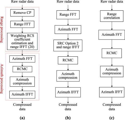
Figure 5: Block diagram of SAR imaging processing: (a) CP based OFDM SAR; (b) LFM SAR; (c) Random noise SAR and conventional OFDM SAR.

The simulation experiments are performed with the following parameters as a typical SAR system: PRF = $800$ Hz, the bandwidth is $B=150$ MHz, the antenna length is $L_{a}=1$ m, the carrier frequency $f_{c}=9$ GHz, the synthetic aperture time is $T_{a}=1$ sec, the effective radar platform velocity is $v_{p}=150$ m/sec, the platform height of the antenna is $H_{p}=5$ km, the slant range swath center is $R_{c}=5\sqrt{2}$ km, the sampling frequency $f_{s}=150$ MHz, the number of range cells is $M=96$ with the center at $R_{c}$. For the convenience of FFT/IFFT computation, we set $T=\frac{512}{150}\ \mu s\approx 3.41\ \mu s$, then the number of subcarriers for the OFDM signal is $N=512$. The CP length is $95$ that is sufficient and the CP time duration is $T_{GI}=\frac{95}{150}\ \mu s\approx 0.63\ \mu s$. Thus, the time duration of an OFDM pulse is $T_{o}=\frac{607}{150}\ \mu s\approx 4.05\ \mu s$. The complex weight vectors over the subcarriers of the CP based OFDM signal and the conventional OFDM signal are set to be vectors of binary PN sequence of values $-1$ and $1$. Meanwhile, for the transmission energies of the three SAR imaging methods to be the same, the time durations of an LFM pulse, a conventional OFDM pulse and a random noise pulse are also $4.05\ \mu s$.

A point target is assumed to be located at the range swath center. Without considering the additive noise, the normalized range profiles of the point spread function are shown in Fig. 6 and the details around the mainlobe area are shown in its zoom-in image. It can be seen that the sidelobes are much lower for the CP based OFDM signal than those of the other three signals, while the $3$ dB mainlobe widths of the four signals are all the same.

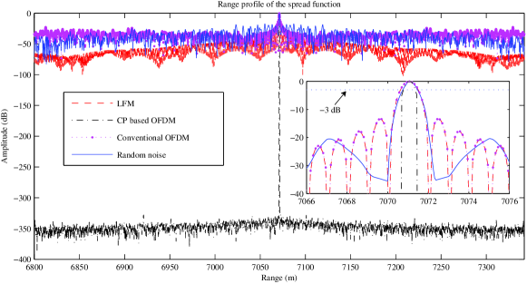
Figure 6: The range profiles of the point spread function.

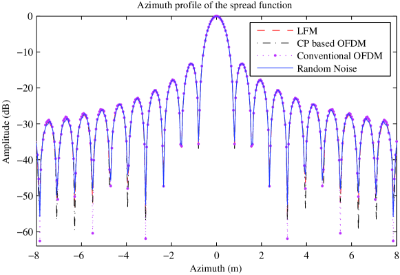
Figure 7: The azimuth profiles of the point spread function.

The normalized azimuth profiles of the point spread function of the three methods are shown in Fig. 7. The results show that the azimuth profiles of the point spread function are similar for all the four signals of LFM, CP based OFDM, conventional OFDM and random noise.

We then consider an extended object with the shape of a tank constructed by a few single point scatterers, and the original reflectivity profile is shown as Fig. 8. The results indicate that the imaging performance using the CP based OFDM SAR is better than the other three signals. Specifically, the boundaries of the extended object are observed less blurred by using the CP based OFDM SAR imaging. In Fig. 8, we also consider the imaging of the tank with our proposed method when the CP length is zero and the transmitted OFDM pulse is the same as the conventional OFDM pulse. As a remark, comparing Fig. 8(e) and Fig. 8(f), one may see that the SAR imaging performance degradation is significant when CP length is zero. This is because our proposed range reconstruction method in the receiver, as mentioned at (15)-(21), is for CP based OFDM SAR imaging and different with the traditional matched filter SAR imaging method. Thus, sufficient CP should be included in the transmitted OFDM pulse to achieve IRCI free range reconstruction.

We next consider the importance of adding a sufficient CP in our proposed CP based OFDM SAR imaging. We consider a single range line (a cross range) with $M=96$ range cells, and targets are included in $18$ range cells, the amplitudes are randomly generated and shown as the red circles in Fig. 9, and the RCS coefficients of the other range cells are set to be zero. The normalized imaging results are shown as the blue asterisks. The results indicate that the imaging is precise when the length of CP is $95$, i.e., sufficient CP length, in Fig. 9(a), the amplitudes of the range cells without targets are lower than $-300$ dB, which are due to the computer numerical errors. With the decrease of the CP length the imaging performance is degraded and the IRCI is increased. Specifically, the zero amplitude range cells become non-zero anymore and some targets are even submerged by the IRCI as shown in Fig. 9(b) and Fig. 9(c). We also show the imaging results with the conventional OFDM SAR image as in Fig. 9(d). The curves in Fig. 9(d) indicate that some targets are submerged by the IRCI from other range cells. In Fig. 9, we notice that, when the CP lengthes are $95$ and $80$ (as in Fig. 9(a) and Fig. 9(b), respectively), the imaging performances of our proposed method outperform the conventional OFDM SAR image in Fig. 9(d). However, the imaging performance with zero length CP is worse than the conventional OFDM SAR image, although they have the same transmitted OFDM waveform, which is again because our proposed range reconstruction method at the receiver is different from the conventional method. It also further indicates that a sufficient CP is important for our proposed CP based OFDM SAR imaging.

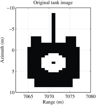
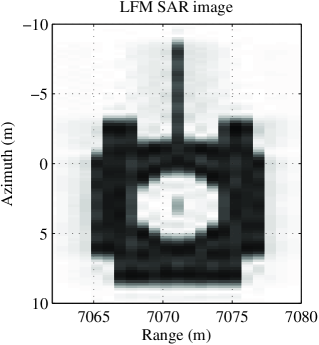
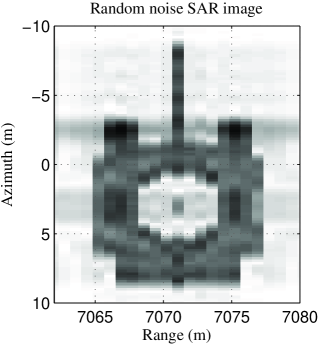
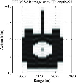
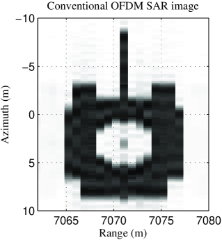
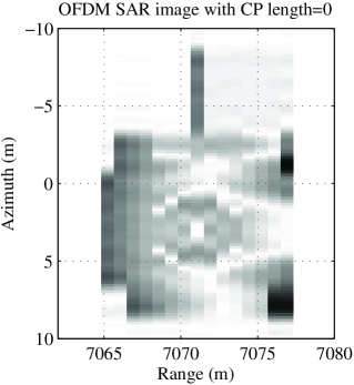
Figure 8: Imaging results of simulated reflectivity profile for a tank: (a) Original tank; (b) LFM SAR; (c) Random noise SAR; (d) OFDM SAR with sufficient CP; (e) Conventional OFDM signal SAR; (f) CP based OFDM SAR with CP length $=0$.

We also consider a single range line (a cross range) with $M$ range cells, in which the RCS coefficients are set $g_{m}=1,\ m=0,\ldots,M-1$. After the CP based OFDM SAR imaging with different lengths of CP, we calculate the mean square errors (MSE) between the energy normalized imaging results and the original RCS coefficients $g_{m}$. The results are achieved from the average of $1000$ independent Monte Carlo simulations and are shown in Fig. 10. The curves suggest that the performance degradation occurs when the length of CP is less than $M-1$, i.e., insufficient. The MSE is supposed to be zero when the CP length is $M-1$ that is sufficient. However, one can still observe some errors in Fig. 10, which is because errors may occur by using a fixed reference range cell $R_{c}$ in the imaging processing (i.e., RCMC and azimuth compression), and the wider swath (or a larger $M$) causes the larger imaging error. Thus, the MSE is slightly larger when $M$ is larger.

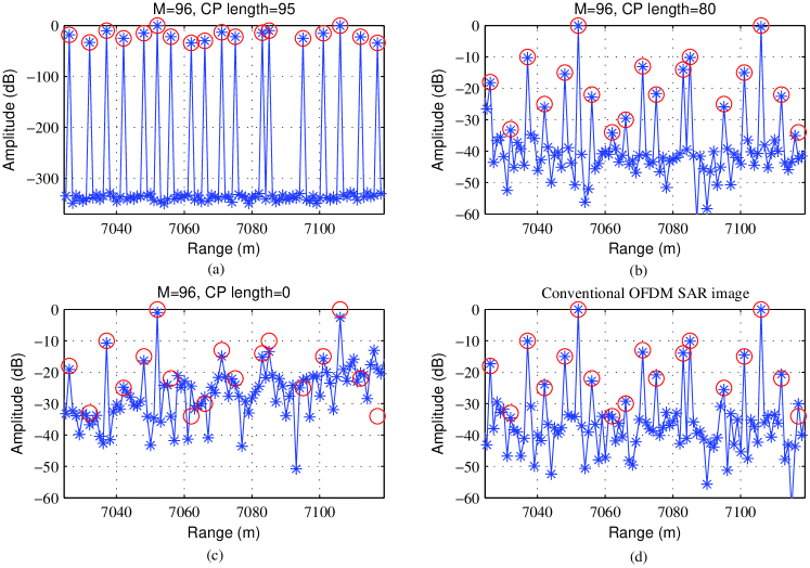
Figure 9: A range line imaging with different CP lengths. Red circles denote the real target amplitudes, blue asterisks denote imaging results.

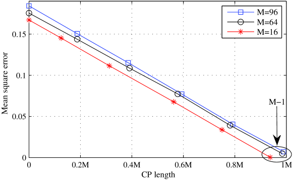
Figure 10: The mean square errors for insufficient CP lengths.

IV Conclusion

In this paper, by using the most important feature of OFDM signals in communications systems, namely converting an ISI channel to multiple ISI-free subchannels, we have proposed a novel method for SAR imaging using OFDM signals with sufficient CP. The sufficient CP insertion provides an IRCI free (high range resolution) SAR image. We first established the CP based OFDM SAR imaging system model and then derived the CP based OFDM SAR imaging algorithm with sufficient CP and showed that this algorithm has zero IRCI (or IRCI-free) for each cross range. We also analyzed the influence when the CP length is insufficient. By comparing with the LFM SAR and the random noise SAR imaging methods, we then finally provided some simulations to illustrate the high range resolution property of the proposed CP based OFDM SAR imaging and also the necessity of a sufficient CP insertion in an OFDM signal. The main features of the proposed SAR imaging are highlighted below.

• The sufficient CP length $M-1$ is determined by the number of range cells $M$ within a swath, which is directly related to the range resolution of the SAR system.

• The optimal time duration of the OFDM pulse is $T_{o}=(2N-1)T_{s}$ with CP length $N-1$. The minimum range of the proposed CP based OFDM SAR is the same as the maximal swath width.

• The range sidelobes are ideally zero for the proposed CP based OFDM SAR imaging, which can provide high range resolution potential for SAR systems. From our simulations, we see that the imaging performance of the CP based OFDM SAR is better than those of the LFM SAR and the random noise SAR, which may be more significant in MIMO radar applications.

• The imaging performance of the CP based OFDM SAR is degraded and the IRCI is increased when the CP length is insufficient.

Some future researches may be needed for our proposed CP based OFDM SAR imaging systems. One of them is the high PAPR problem of the OFDM signals as what has been pointed out in Section II-C. Another problem is that OFDM signals are sensitive to an unknown Doppler shift, such as, that induced from an known moving target, which may damage the orthogonality of OFDM subcarriers and result in the potential ICI. Also, how does our proposed OFDM SAR imaging method work for a distributed target model [39]? Some of these problems are under our current investigations.

References

- [1] N. C. Currie, Radar Reflectivity Measurement: Techniques and Applications. Norwood, MA: Artech House, 1989.
- [2] M. Soumekh, Synthetic Aperture Radar Signal Processing. New York: Wiley, 1999.
- [3] S. R. J. Axelsson, “Analysis of random step frequency radar and comparison with experiments,” Geoscience and Remote Sensing, IEEE Transactions on, vol. 45, no. 4, pp. 890–904, 2007.
- [4] X. Xu and R. Narayanan, “FOPEN SAR imaging using UWB step-frequency and random noise waveforms,” Aerospace and Electronic Systems, IEEE Transactions on, vol. 37, no. 4, pp. 1287–1300, 2001.
- [5] D. Garmatyuk and R. Narayanan, “Ultra-wideband continuous-wave random noise arc-SAR,” Geoscience and Remote Sensing, IEEE Transactions on, vol. 40, no. 12, pp. 2543–2552, 2002.
- [6] G.-S. Liu, H. Gu, W.-M. Su, H.-B. Sun, and J.-H. Zhang, “Random signal radar - a winner in both the military and civilian operating environments,” Aerospace and Electronic Systems, IEEE Transactions on, vol. 39, no. 2, pp. 489–498, 2003.
- [7] N. Levanon, “Multifrequency complementary phase-coded radar signal,” Radar, Sonar and Navigation, IEE Proceedings, vol. 147, no. 6, pp. 276–284, 2000.
- [8] G. E. A. Franken, H. Nikookar, and P. van Genderen, “Doppler tolerance of OFDM-coded radar signals,” in Radar Conference, 2006. EuRAD 2006. 3rd European, Manchester, UK, 2006, pp. 108–111.
- [9] D. Garmatyuk and J. Schuerger, “Conceptual design of a dual-use radar/communication system based on OFDM,” in Military Communications Conference, 2008. MILCOM 2008. IEEE, San Diego, CA, 2008, pp. 1–7.
- [10] D. Garmatyuk, J. Schuerger, K. Kauffman, and S. Spalding, “Wideband OFDM system for radar and communications,” in Radar Conference, 2009 IEEE, Pasadena, CA, 2009, pp. 1–6.
- [11] C. Sturm, E. Pancera, T. Zwick, and W. Wiesbeck, “A novel approach to OFDM radar processing,” in Radar Conference, 2009 IEEE, Pasadena, CA, 2009, pp. 1–4.
- [12] Y. L. Sit, C. Sturm, L. Reichardt, T. Zwick, and W. Wiesbeck, “The OFDM joint radar-communication system: An overview,” in SPACOMM 2011, The Third International Conference on Advances in Satellite and Space Communications, Budapest, Hungary, 2011, pp. 69–74.
- [13] C. Sturm and W. Wiesbeck, “Waveform design and signal processing aspects for fusion of wireless communications and radar sensing,” Proceedings of the IEEE, vol. 99, no. 7, pp. 1236–1259, 2011.
- [14] S. Sen and A. Nehorai, “Target detection in clutter using adaptive OFDM radar,” Signal Processing Letters, IEEE, vol. 16, no. 7, pp. 592–595, 2009.
- [15] ——, “Adaptive design of OFDM radar signal with improved wideband ambiguity function,” Signal Processing, IEEE Transactions on, vol. 58, no. 2, pp. 928–933, 2010.
- [16] ——, “OFDM MIMO radar with mutual-information waveform design for low-grazing angle tracking,” Signal Processing, IEEE Transactions on, vol. 58, no. 6, pp. 3152–3162, 2010.
- [17] V. Riche, S. Meric, J. Baudais, and E. Pottier, “Optimization of OFDM SAR signals for range ambiguity suppression,” in Radar Conference (EuRAD), 2012 9th European, Amsterdam, Netherlands, 2012, pp. 278–281.
- [18] V. Riche, S. Meric, E. Pottier, and J.-Y. Baudais, “OFDM signal design for range ambiguity suppression in SAR configuration,” in Geoscience and Remote Sensing Symposium (IGARSS), 2012 IEEE International, Munich, Germany, 2012, pp. 2156–2159.
- [19] V. Riche, S. Meric, J.-Y. Baudais, and E. Pottier, “Investigations on OFDM signal for range ambiguity suppression in SAR configuration,” Geoscience and Remote Sensing, IEEE Transactions on, vol. 52, no. 7, pp. 4194–4197, 2014.
- [20] J.-H. Kim, M. Younis, A. Moreira, and W. Wiesbeck, “A novel OFDM chirp waveform scheme for use of multiple transmitters in SAR,” Geoscience and Remote Sensing Letters, IEEE, vol. 10, no. 3, pp. 568–572, 2013.
- [21] D. Garmatyuk, “Simulated imaging performance of UWB SAR based on OFDM,” in Ultra-Wideband, The 2006 IEEE 2006 International Conference on, Waltham, MA, 2006, pp. 237–242.
- [22] D. Garmatyuk and M. Brenneman, “Adaptive multicarrier OFDM SAR signal processing,” Geoscience and Remote Sensing, IEEE Transactions on, vol. 49, no. 10, pp. 3780–3790, 2011.
- [23] D. Garmatyuk, “Cross-range SAR reconstruction with multicarrier OFDM signals,” Geoscience and Remote Sensing Letters, IEEE, vol. 9, no. 5, pp. 808–812, 2012.
- [24] C. Berger, B. Demissie, J. Heckenbach, P. Willett, and S. Zhou, “Signal processing for passive radar using OFDM waveforms,” Selected Topics in Signal Processing, IEEE Journal of, vol. 4, no. 1, pp. 226–238, 2010.
- [25] F. Colone, K. Woodbridge, H. Guo, D. Mason, and C. Baker, “Ambiguity function analysis of wireless LAN transmissions for passive radar,” Aerospace and Electronic Systems, IEEE Transactions on, vol. 47, no. 1, pp. 240–264, 2011.
- [26] J. R. Gutierrez Del Arroyo and J. A. Jackson, “WiMAX OFDM for passive SAR ground imaging,” Aerospace and Electronic Systems, IEEE Transactions on, vol. 49, no. 2, pp. 945–959, 2013.
- [27] P. Falcone, F. Colone, C. Bongioanni, and P. Lombardo, “Experimental results for OFDM WiFi-based passive bistatic radar,” in Radar Conference, 2010 IEEE, Washington, D.C., 2010, pp. 516–521.
- [28] F. Colone, P. Falcone, and P. Lombardo, “Ambiguity function analysis of WiMAX transmissions for passive radar,” in Radar Conference, 2010 IEEE, Washington, D.C., 2010, pp. 689–694.
- [29] K. Chetty, K. Woodbridge, H. Guo, and G. Smith, “Passive bistatic WiMAX radar for marine surveillance,” in Radar Conference, 2010 IEEE, Washington, D.C., 2010, pp. 188–193.
- [30] Q. Wang, C. Hou, and Y. Lu, “WiMAX signal waveform analysis for passive radar application,” in Radar Conference - Surveillance for a Safer World, 2009. RADAR. International, Bordeaux, France, 2009, pp. 1–6.
- [31] M. I. Skolnik, Introduction to Radar Systems. New York, USA: McGraw-Hill, 2001.
- [32] X.-G. Xia, “Discrete chirp-Fourier transform and its application to chirp rate estimation,” Signal Processing, IEEE Transactions on, vol. 48, no. 11, pp. 3122–3133, 2000.
- [33] R. Prasad, OFDM for Wireless Communications Systems. Artech House Publishers, Boston, 2004.
- [34] E. Dahlman, S. Parkvall, and J. Skold, 4G: LTE/LTE-Advanced for Mobile Broadband. Academic Press, New York, 2011.
- [35] A. Goldsmith, Wireless Communications. Cambridge University Press, New York, 2005.
- [36] M. Suess, B. Grafmueller, and R. Zahn, “A novel high resolution, wide swath SAR system,” in Geoscience and Remote Sensing Symposium, IGARSS, Sydney, Australia, 2001, pp. 1013–1015.
- [37] S. Beyme and C. Leung, “Efficient computation of DFT of Zadoff-Chu sequences,” Electronics Letters, vol. 45, no. 9, pp. 461–463, 2009.
- [38] B. Popovic, “Efficient DFT of Zadoff-Chu sequences,” Electronics Letters, vol. 46, no. 7, pp. 502–503, 2010.
- [39] G. Krieger, “MIMO-SAR: Opportunities and pitfalls,” Geoscience and Remote Sensing, IEEE Transactions on, vol. 52, no. 5, pp. 2628–2645, 2014.