Accurate and efficient approximation to the optimized effective potential for exchange

Abstract

We devise an efficient practical method for computing the Kohn–Sham exchange-correlation potential corresponding to a Hartree–Fock electron density. This potential is almost indistinguishable from the exact-exchange optimized effective potential (OEP) and, when used as an approximation to the OEP, is vastly better than all existing models. Using our method one can obtain unambiguous, nearly exact OEPs for any finite one-electron basis set at the same low cost as the Krieger–Li–Iafrate and Becke–Johnson potentials. For all practical purposes, this solves the long-standing problem of black-box construction of OEPs in exact-exchange calculations.

The purpose of this Letter is to suggest an essentially exact, robust, practical method for constructing the optimized effective potential (OEP) Grabo et al. (2000) of the exact-exchange Kohn–Sham scheme. OEPs naturally arise in the theory of orbital-dependent functionals Kümmel and Kronik (2008)—one of the most promising modern density-functional techniques—and are of significant practical interest because they afford qualitatively better description of molecular properties than local and semilocal approximations Grabo et al. (2000); Kümmel and Kronik (2008).

The exchange-only OEP is defined Sharp and Horton (1953) as the multiplicative potential $v_{\text{X}}^{\text{OEP}}(\mathbf{r})$ that minimizes the Hartree–Fock (HF) total energy expression within the Kohn–Sham scheme. Equivalently Sahni et al. (1982), the OEP is the functional derivative $v_{\text{X}}^{\text{OEP}}(\mathbf{r})\equiv\delta E_{\text{X}}^{\text{exact}}/\delta\rho(\mathbf{r})$, where $E_{\text{X}}^{\text{exact}}$ is the HF exchange energy expression written in terms of Kohn–Sham orbitals (an implicit density functional) and $\rho(\mathbf{r})$ is the electron density. To obtain $v_{\text{X}}^{\text{OEP}}(\mathbf{r})$ in a formally correct manner, one has to solve the OEP integral equation Grabo et al. (2000). Unfortunately, every attempt to do this runs into severe numerical difficulties because the problem is ill-posed Hirata et al. (2001) and has infinitely many solutions in finite basis sets Hirata et al. (2001); Staroverov et al. (2006a). Recent advances in OEP methods Kümmel and Perdew (2003); Heßelmann et al. (2007); Görling et al. (2008); Heaton-Burgess et al. (2007); Kollmar and Filatov (2007, 2008); Jacob (2011); Gidopoulos and Lathiotakis (2012) have alleviated some of these difficulties but, even today, flawless OEPs can be obtained only case by case, with painstaking effort.

In the absence of an efficient OEP solver, various approximations to the OEP have long been used as pragmatic alternatives. These include the Krieger–Li–Iafrate (KLI) Krieger et al. (1992), localized Hartree–Fock (LHF) Della Sala and Görling (2001), and related approximations Grüning et al. (2002); Holas and Cinal (2005); Staroverov et al. (2006b); Izmaylov et al. (2007), as well as model potentials for exact exchange van Leeuwen et al. (1996); Gritsenko et al. (1999); Becke and Johnson (2006); Staroverov (2008); Räsänen et al. (2010), of which the Becke–Johnson (BJ) approximation Becke and Johnson (2006) is the most popular. The LHF method is equivalent Izmaylov et al. (2007) to the common energy denominator approximation (CEDA) Grüning et al. (2002) and to the effective local potential (ELP) scheme Staroverov et al. (2006b).

In a parallel development, several workers studied Payne (1979); Holas et al. (1993); Görling and Ernzerhof (1995); Holas and March (1996) the HF method as a density-functional problem and occasionally observed Chen et al. (1994); Filippi et al. (1996) that Kohn–Sham exchange-correlation potentials corresponding to HF electron densities (HFXC potentials for short) were very close to OEPs. However, this observation had little impact on the OEP impasse because existing methods for determining exchange-correlation potentials from densities (see, for instance, Refs. Zhao et al., 1994; van Leeuwen and Baerends, 1994; Tozer et al., 1996; Wu and Yang, 2003a; Ryabinkin and Staroverov, 2012) face the same basis-set artifacts Schipper et al. (1997) and numerical challenges Bulat et al. (2007) as attempts to solve the OEP equation.

In this work, we devise a practical, artifact-free procedure which allows one to compute the HFXC potential efficiently for any atom or molecule. Then we use our method to show, on a variety of systems, that HFXC potentials are not just close but practically indistinguishable from OEPs. The significance of our approach is that it has the same reliability and computational cost as the KLI, LHF, and BJ schemes, but its accuracy is vastly superior.

The proposed method originated with our observation that the quantity $(\tau^{\text{HF}}-\tau)/\rho$, where $\tau$ and $\tau^{\text{HF}}$ are the Kohn–Sham and HF kinetic energy densities, reproduces that part of atomic shell structure of exact-exchange potentials which is missing in the KLI and LHF approximations. While searching for a rigorous explanation, we realized that we were dealing with the HFXC potential and arrived at the following argument.

Consider the HF description of a closed-shell $N$-electron system. The exchange energy of this system is

$$E_{\text{X}}^{\text{HF}}=-\frac{1}{4}\int d\mathbf{r}\int\frac{|\gamma^{\text{HF}}(\mathbf{r},\mathbf{r}^{\prime})|^{2}}{|\mathbf{r}-\mathbf{r}^{\prime}|}\,d\mathbf{r}^{\prime},$$ (1)

where $\gamma^{\text{HF}}(\mathbf{r},\mathbf{r}^{\prime})=\sum_{i=1}^{N}\phi_{i}^{\text{HF}}(\mathbf{r})\phi_{i}^{\text{HF}*}(\mathbf{r}^{\prime})$ is the spinless reduced density matrix and $\phi_{i}^{\text{HF}}$ is the spatial part of the $i$th canonical HF spin-orbital. The HF electron density is given by $\rho^{\text{HF}}(\mathbf{r})=\sum_{i=1}^{N}|\phi_{i}^{\text{HF}}(\mathbf{r})|^{2}$. The orbitals $\phi_{i}^{\text{HF}}$ are the lowest-eigenvalue solutions of the HF equations

$$\left[-\dfrac{1}{2}\nabla^{2}+v(\mathbf{r})+v_{\text{H}}(\mathbf{r})+\hat{K}\right]\phi_{i}^{\text{HF}}(\mathbf{r})=\epsilon_{i}^{\text{HF}}\phi_{i}^{\text{HF}}(\mathbf{r}),$$ (2)

where $v(\mathbf{r})$ is the external potential (e.g., the potential of the nuclei), $v_{\text{H}}(\mathbf{r})=\int\rho^{\text{HF}}(\mathbf{r}^{\prime})|\mathbf{r}-\mathbf{r}^{\prime}|^{-1}\,d\mathbf{r}^{\prime}$ is the Hartree (electrostatic) potential of $\rho^{\text{HF}}(\mathbf{r})$, and $\hat{K}$ is the Fock exchange operator defined by

$$\hat{K}\phi_{i}^{\text{HF}}(\mathbf{r})=\frac{\delta E_{\text{X}}^{\text{HF}}}{\delta\phi_{i}^{\text{HF}*}(\mathbf{r})}=-\frac{1}{2}\int\frac{\gamma^{\text{HF}}(\mathbf{r},\mathbf{r}^{\prime})}{|\mathbf{r}-\mathbf{r}^{\prime}|}\phi_{i}^{\text{HF}}(\mathbf{r}^{\prime})\,d\mathbf{r}^{\prime}.$$ (3)

Let us multiply Eq. (2) by $\phi_{i}^{\text{HF}*}$, sum over $i$ from 1 to $N$, and divide through by $\rho^{\text{HF}}$. The result is

$$\frac{\tau_{L}^{\text{HF}}}{\rho^{\text{HF}}}+v+v_{\text{H}}+v_{\text{S}}^{\text{HF}}=\frac{1}{\rho^{\text{HF}}}\sum_{i=1}^{N}\epsilon_{i}^{\text{HF}}|\phi_{i}^{\text{HF}}|^{2},$$ (4)

where $\tau_{L}^{\text{HF}}(\mathbf{r})=-\frac{1}{2}\sum_{i=1}^{N}\phi_{i}^{\text{HF*}}(\mathbf{r})\nabla^{2}\phi_{i}^{\text{HF}}(\mathbf{r})$ is the Laplacian form of the HF kinetic energy density and

$$v_{\text{S}}^{\text{HF}}(\mathbf{r})=-\frac{1}{2\rho^{\text{HF}}(\mathbf{r})}\int\frac{|\gamma^{\text{HF}}(\mathbf{r},\mathbf{r}^{\prime})|^{2}}{|\mathbf{r}-\mathbf{r}^{\prime}|}\,d\mathbf{r}^{\prime}.$$ (5)

is the Slater potential (the orbital-averaged $\hat{K}$ operator) Slater (1951) built from the HF orbitals. The quantity on the right-hand side of Eq. (4) is known as the HF average local ionization energy Bulat et al. (2009),

$$\bar{I}^{\text{HF}}(\mathbf{r})=\frac{1}{\rho^{\text{HF}}(\mathbf{r})}\sum_{i=1}^{N}\epsilon_{i}^{\text{HF}}|\phi_{i}^{\text{HF}}(\mathbf{r})|^{2}.$$ (6)

Note that $\tau_{L}^{\text{HF}}=\tau^{\text{HF}}-\frac{1}{4}\nabla^{2}\rho^{\text{HF}}$, where

$$\tau^{\text{HF}}(\mathbf{r})=\frac{1}{2}\sum_{i=1}^{N}|\nabla\phi_{i}^{\text{HF}}(\mathbf{r})|^{2}$$ (7)

is the positive-definite form of the HF kinetic energy density. In practical calculations, it is much better to deal with $\tau^{\text{HF}}$ than with $\tau_{L}^{\text{HF}}$ because the former is always finite, whereas the latter becomes infinite at the nuclei. With these definitions we rewrite Eq. (4) as

$$\frac{\tau^{\text{HF}}}{\rho^{\text{HF}}}-\frac{1}{4}\frac{\nabla^{2}\rho^{\text{HF}}}{\rho^{\text{HF}}}+v+v_{\text{H}}+v_{\text{S}}^{\text{HF}}=\bar{I}^{\text{HF}}.$$ (8)

Now, let us pose the following problem: Find the multiplicative exchange-correlation potential of the Kohn–Sham scheme which generates the same electron density as the HF method. This HFXC potential, $v_{\text{XC}}^{\text{HF}}(\mathbf{r})$, is defined by the Kohn–Sham equations

$$\left[-\dfrac{1}{2}\nabla^{2}+v(\mathbf{r})+v_{\text{H}}(\mathbf{r})+v_{\text{XC}}^{\text{HF}}(\mathbf{r})\right]\phi_{i}(\mathbf{r})=\epsilon_{i}\phi_{i}(\mathbf{r}),$$ (9)

where $v$ and $v_{\text{H}}$ are the same as in Eq. (2) and the eigenfunctions $\phi_{i}$ are such that $\rho(\mathbf{r})\equiv\sum_{i=1}^{N}|\phi_{i}(\mathbf{r})|^{2}=\rho^{\text{HF}}(\mathbf{r})$. An important point here is that the equality $\rho=\rho^{\text{HF}}$ does not imply that $\phi_{i}=\phi_{i}^{\text{HF}}$. In fact, the canonical orbitals $\phi_{i}$ and $\phi_{i}^{\text{HF}}$ are known to be slightly different Görling and Ernzerhof (1995).

To find $v_{\text{XC}}^{\text{HF}}(\mathbf{r})$, we perform the same manipulations on Eq. (9) that led from Eq. (2) to Eq. (8) and arrive at

$$\frac{\tau}{\rho}-\frac{1}{4}\frac{\nabla^{2}\rho}{\rho}+v+v_{\text{H}}+v_{\text{XC}}^{\text{HF}}=\bar{I},$$ (10)

where $\tau(\mathbf{r})=\frac{1}{2}\sum_{i=1}^{N}|\nabla\phi_{i}(\mathbf{r})|^{2}$ is the positive-definite Kohn–Sham kinetic energy density, and

$$\bar{I}(\mathbf{r})=\frac{1}{\rho(\mathbf{r})}\sum_{i=1}^{N}\epsilon_{i}|\phi_{i}(\mathbf{r})|^{2}$$ (11)

is the Kohn–Sham average local ionization energy. Finally, we subtract Eq. (8) from (10) and write

$$v_{\text{XC}}^{\text{HF}}(\mathbf{r}) =v_{\text{S}}^{\text{HF}}(\mathbf{r})+\bar{I}(\mathbf{r})-\bar{I}^{\text{HF}}(\mathbf{r})+\frac{\tau^{\text{HF}}(\mathbf{r})}{\rho^{\text{HF}}(\mathbf{r})}-\frac{\tau(\mathbf{r})}{\rho(\mathbf{r})},$$ (12)

where $\rho=\rho^{\text{HF}}$, but $\tau\neq\tau^{\text{HF}}$ and $\bar{I}\neq\bar{I}^{\text{HF}}$.

Equation (12) is the key result of this work. It gives the HFXC potential exactly (in a complete basis). Analogous but less practical expressions for $v_{\text{XC}}^{\text{HF}}$ were presented earlier in Refs. Holas and March, 1997; Nagy, 1997; Miao, 2000.

We propose to treat Eq. (12) as the definition of a model Kohn–Sham potential for exact exchange. To turn this definition into a practical method we observe that $\bar{I}$ and $\tau$ are determined by $v_{\text{XC}}^{\text{HF}}$ and hence are initially unknown. Therefore, Eq. (12) has to be solved iteratively. The algorithm we suggest is as follows.

1. Perform an HF calculation on the system of interest and construct $\rho^{\text{HF}}$, $v_{\text{S}}^{\text{HF}}$, $\tau^{\text{HF}}$, and $\bar{I}^{\text{HF}}$.

2. Choose an initial guess for the occupied Kohn–Sham orbitals $\{\phi_{i}\}$ and their eigenvalues $\{\epsilon_{i}\}$ (e.g., HF orbitals and orbital energies).

3. Shift all $\epsilon_{i}$ simultaneously to satisfy the condition $\epsilon_{N}=\epsilon_{N}^{\text{HF}}$. This is needed to ensure that $v_{\text{XC}}^{\text{HF}}$ retains the correct $-1/r$ asymptotic behavior of $v_{\text{S}}^{\text{HF}}$.

4. Construct $v_{\text{XC}}^{\text{HF}}$ by substituting the current $\{\phi_{i}\}$ and $\{\epsilon_{i}\}$ into Eq. (12). To facilitate convergence, we found it essential to compute the terms $\bar{I}$ and $\tau/\rho$ using the density $\rho=\sum_{i=1}^{N}|\phi_{i}|^{2}$ rather than $\rho^{\text{HF}}$.

5. Solve the Kohn–Sham equations (9) using the current $v_{\text{XC}}^{\text{HF}}$. This gives a new set of $\{\phi_{i}\}$ and $\{\epsilon_{i}\}$.

6. Return to Step 3. Iterate until $v_{\text{XC}}^{\text{HF}}$ is self-consistent, i.e., until $\{\phi_{i}\}$ and $\{\epsilon_{i}\}$ on input and output agree within a desired threshold.

For spin-polarized systems, there will be two HFXC potentials (spin-up and spin-down) and hence two sets of all quantities except $v$ and $v_{\text{H}}$. The entire scheme described above was implemented in gaussian 09 G (09).

The most computationally intensive step in the HFXC approach, as in the KLI, LHF, BJ, and related approximations, is the construction of the Slater potential. It helps that in our method the Slater potential has to be computed only once (at the start of iterations). To eliminate every possible source of errors unrelated to the HFXC approximation, here we constructed $v_{\text{S}}^{\text{HF}}(\mathbf{r})$ by using Eq. (5). For routine applications, we recommend resolution-of-the-identity techniques or the method of Ref. Kananenka et al., .

To assess the quality of HFXC potentials produced by our method we compared them to the exact (numerical) OEPs, some of the best existing OEP approximations (KLI, ELP=LHF=CEDA, and BJ), and finite-basis-set OEPs obtained by the Wu–Yang OEP (WY-OEP) method Wu and Yang (2003b). The OEP and KLI results were taken from the work of Engel and coworkers Engel and Vosko (1993); Engel and Dreizler (1999); Engel (for spherical atoms) and from Makmal et al. Makmal et al. (2009) (for molecules); these are exact fully numerical solutions of the OEP and KLI equations. The BJ, ELP, and WY-OEP results were obtained earlier by one of the authors Gaiduk and Staroverov (2008). To simulate the basis-set limit in the HFXC, BJ, ELP, and WY-OEP calculations we employed the large universal Gaussian basis set (UGBS) of Ref. de Castro and Jorge, 1998 for atoms and UGBS1P (UGBS augmented with one set of polarization functions for each exponent) for molecules. The accuracy of the UGBS is such that total atomic HF energies computed in this basis are converged to 7 significant figures with respect to the basis-set limit de Castro and Jorge (1998).

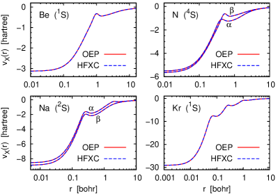
Figure 1: OEPs and HFXC potentials are visually indistinguishable. The same excellent agreement was observed for all atoms where comparison with OEPs was made.

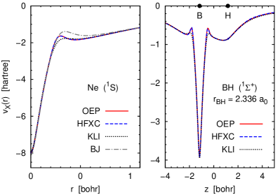
Figure 2: HFXC potentials are perfect representations of OEPs, unlike KLI and BJ potentials. The potentials for the BH molecule are shown along the internuclear axis.

In all cases where the UGBS (UGBS1P) was used, we found that HFXC potentials are virtually indistinguishable from exact OEPs (Figs. 1 and 2) and are dramatically better as approximations to OEPs than the KLI and BJ models (Fig. 2). Note that the performance of the LHF approximation is very similar to that of the KLI Della Sala and Görling (2001) scheme, so the LHF or ELP or CEDA curves (not shown in Fig. 2) would be almost superimposed with the KLI potentials. The excellent agreement between HFXC potentials and exact OEPs suggests that the ‘correlation’ part of an HFXC potential is negligibly small.

For quantitative comparison, we took the self-consistent Kohn–Sham orbitals generated by HFXC and other potentials and calculated the conventional total exchange-only energy, $E_{\text{conv}}$, which defined as the HF total energy expression in terms of Kohn–Sham orbitals. Table 1 shows that the KLI, ELP, and BJ potentials produce $E_{\text{conv}}$ values noticeably above the exact OEP energies. By contrast, conventional energies obtained from HFXC potentials are within 0.1 m$E_{\text{h}}$ of the OEP benchmarks for most atoms—closer than $E_{\text{conv}}$ values from WY-OEPs.

Table 1: Total ground-state energies of 12 representative atoms obtained with various exchange potentials. The numerical OEP and KLI results are from Refs. Engel and Vosko, 1993; Engel and Dreizler, 1999; Engel, . All other values were computed using a large Gaussian basis set (UGBS).

	$E_{\text{OEP}}$	$E_{\text{conv}}-E_{\text{OEP}}$ (units of m$E_{\text{h}}$)					$E_{\text{vir}}-E_{\text{conv}}$ (units of m$E_{\text{h}}$)
Atom	(units of $E_{\text{h}}$)	KLI	ELP	BJ	WY-OEP	HFXC	KLI	ELP	BJ	WY-OEP	HFXC
Li	$-7.43250$	$0.06$	$0.08$	$1.20$	$0.00$	$0.00$	$-5.28$	$4.61$	$50.45$	$-0.01$	$-0.04$
Be	$-14.57243$	$0.15$	$0.15$	$0.75$	$0.01$	$-0.01$	$-21.20$	$13.85$	$31.68$	$0.07$	$-0.10$
N	$-54.40340$	$0.36$	$0.34$	$4.14$	$0.01$	$0.00$	$24.74$	$78.47$	$250.56$	$-0.04$	$-0.21$
Ne	$-128.54541$	$0.58$	$0.57$	$9.59$	$0.02$	$0.01$	$155.62$	$197.51$	$781.68$	$-0.05$	$-0.14$
Na	$-161.85664$	$0.73$	$0.73$	$7.71$	$0.02$	$0.00$	$183.10$	$231.84$	$805.90$	$0.22$	$-0.28$
Mg	$-199.61158$	$0.87$	$0.87$	$5.86$	$0.02$	$0.00$	$182.26$	$267.70$	$799.35$	$-0.64$	$-0.26$
P	$-340.71500$	$1.28$	$1.28$	$3.99$	$0.02$	$-0.03$	$144.86$	$376.08$	$904.12$	$1.21$	$-1.84$
Ar	$-526.81222$	$1.74$	$1.83$	$3.36$	$0.09$	$-0.07$	$124.68$	$512.68$	$1182.26$	$2.54$	$-4.08$
Ca	$-676.75193$	$2.23$	$1.98$	$3.58$	$-0.03$	$-0.13$	$14.94$	$597.73$	$1126.91$	$-2.49$	$-5.86$
Zn	$-1777.83436$	$3.65$	$3.05$	$10.40$	$-0.07$	$-0.07$	$1047.87$	$1238.61$	$2130.22$	$-1.21$	$-5.93$
Kr	$-2752.04295$	$3.18$	$3.44$	$6.52$	$0.26$	$-0.07$	$1468.11$	$1657.32$	$3128.48$	$7.85$	$-7.43$
Cd	$-5465.11441$	$6.04$	$5.58$	$6.46$	$0.92$	$-0.26$	$1883.92$	$2374.14$	$3617.48$	$-4.25$	$-6.99$
m.a.v.		$1.74$	$1.66$	$5.30$	$0.12$	$0.05$	$438.0$	$629.2$	$1234.1$	$1.76$	$2.76$

A more stringent quality test Gaiduk and Staroverov (2008) for OEP approximations is the virial energy discrepancy, $\Delta_{\text{vir}}=E_{\text{vir}}-E_{\text{conv}}$, where $E_{\text{vir}}$ is the total energy with the exchange contribution obtained by the Levy–Perdew virial relation Levy and Perdew (1985),

$$E_{\text{X}}^{\text{vir}}=\int v_{\text{X}}(\mathbf{r})\left[3\rho(\mathbf{r})+\mathbf{r}\cdot\nabla\rho(\mathbf{r})\right]d\mathbf{r}.$$ (13)

For exact OEPs, $\Delta_{\text{vir}}=0$ Ou-Yang and Levy (1990). Table 1 shows that virial energy discrepancies for HFXC potentials do not exceed a few m$E_{\text{h}}$, that is, are three orders of magnitude smaller than for the LHF, ELP, and BJ approximations—as small as for WY-OEPs. These discrepancies are expected to be even smaller in the basis-set limit. (The numerical OEPs have $\Delta_{\text{vir}}$ values of the order of a few $\mu E_{\text{h}}$ Engel .)

Recall that to solve the OEP integral equation by the WY method one needs two sets of basis functions: a one-electron basis for the orbitals and an auxiliary basis for the OEP. The two sets must be “balanced” with respect to each other; otherwise, the resulting potential will be either suboptimal or highly oscillatory Staroverov et al. (2006a); Heßelmann et al. (2007); Görling et al. (2008); Heaton-Burgess et al. (2007). By employing the same large basis set in both roles one can usually Staroverov et al. (2006a) obtain OEPs that are smooth and correct everywhere except near the nucleus (the left panel in Fig. 3). However, the single-basis trick does not work for small and medium-sized one-electron basis sets such as 6-31G and cc-pVQZ, for which a suitable auxiliary basis can be found only in an ad hoc manner with considerable effort and some arbitrariness Heßelmann et al. (2007); Görling et al. (2008); Heaton-Burgess et al. (2007). Such problems do not exist in our method, where we automatically obtain a smooth HFXC potential for any one-electron basis (the right panel in Fig. 3). Since OEPs and HFXC potentials are nearly identical in the basis-set limit, one can even operationally define a finite-basis-set OEP (a fundamentally ambiguous quantity Staroverov et al. (2006a)) as the corresponding HFXC potential.

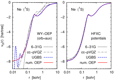
Figure 3: WY-OEPs and HFXC potentials obtained with small (6-31G), intermediate (cc-pVQZ), and large (UGBS) basis sets as approximations to the exact (numerical) OEP. The HFXC/UGBS curve is right on top of the OEP.

The reason the HFXC scheme is very robust is because the potential $v_{\text{XC}}^{\text{HF}}$ is built up directly as a sum of commensurate, well-behaved terms. Apart from being a tool for generating approximate OEPs, the HFXC method can be used to determine Kohn–Sham potentials from HF densities, provided that the HF and Kohn–Sham orbitals are expanded in a complete (in practice, very large) basis or represented on a dense grid. In Kohn–Sham calculations using a finite basis set, however, the potential given by Eq. (12) reproduces the target $\rho^{\text{HF}}(\mathbf{r})$ only approximately because Eq. (9) and its finite-dimensional matrix representation are not equivalent foo .

We can also identify the reason why HFXC potentials are much closer to OEPs than KLI, LHF, and related approximations. This happens because in our derivation we did not assume that $\phi_{i}=\phi_{i}^{\text{HF}}$ for all $i\leq N$. If, for the sake of argument, we make this assumption in Eq. (12), we immediately obtain a different potential,

$$\tilde{v}_{\text{XC}}(\mathbf{r})=v_{\text{S}}^{\text{HF}}(\mathbf{r})+\frac{1}{\rho^{\text{HF}}(\mathbf{r})}\sum_{i=1}^{N}(\epsilon_{i}-\epsilon_{i}^{\text{HF}})|\phi_{i}^{\text{HF}}(\mathbf{r})|^{2},$$ (14)

which was introduced and discussed by Nagy Nagy (1997) (with $\phi_{i}$ in place of $\phi_{i}^{\text{HF}}$) as an approximate equivalent of the KLI potential. The difference between HF and OEP orbitals may be small, but it gives rise to the crucial $(\tau^{\text{HF}}-\tau)/\rho$ term responsible for the atomic shell structure of the OEP. It follows that the KLI and LHF approximations would be greatly improved simply by including this term.

In conclusion, we have shown (a) how to construct HFXC potentials (i.e., model exchange-correlation potentials yielding HF densities in the basis-set limit) at the computational cost of the KLI, LHF, and BJ approximations; (b) that HFXC potentials are nearly exact approximations to exchange-only OEPs, much better than the KLI, LHF, BJ, and related models. The advantage of approximating OEPs with HFXC potentials is that it the HFXC method completely avoids the OEP equation, and so is free from numerical difficulties and basis-set artifacts that beset OEP techniques.

HFXC potentials obtained in finite basis sets exhibit no spurious oscillations and, for all intents and purposes, may be treated as solutions of the OEP equation. In this sense, the HFXC scheme solves the long-standing problem of unambiguous “black-box” construction of elusive finite-basis-set OEPs. We anticipate that our approach will be widely embraced as a practical substitute for OEP methods and as a superior alternative to existing model potentials for exact exchange.

Finally, we wish to remark that our approach can be generalized to any orbital-dependent exchange-correlation functional. One simply needs to start with the corresponding energy expression $E_{\text{XC}}[\{\phi_{i}\}]$ instead of $E_{\text{X}}^{\text{HF}}$ and modify appropriately all the steps in the derivation. For $\tau$-dependent functionals and hybrids (mixtures of exact exchange and semilocal approximations), this scheme is expected to produce even more accurate approximations to $\delta E_{\text{XC}}[\{\phi_{i}\}]/\delta\rho$ than for the exact-exchange functional itself.

The authors thank Profs. Eberhard Engel and Leeor Kronik for providing the OEP and KLI benchmarks. I.G.R. is grateful to Dr. Alex Gaiduk for help with the gaussian code. This work was supported by the Natural Sciences and Engineering Research Council of Canada (NSERC) through the Discovery Grants Program.

References

- Grabo et al. (2000) T. Grabo, T. Kreibich, S. Kurth, and E. K. U. Gross, in Strong Coulomb Correlations in Electronic Structure Calculations: Beyond the Local Density Approximation, edited by V. I. Anisimov (Gordon and Breach, Amsterdam, 2000).
- Kümmel and Kronik (2008) S. Kümmel and L. Kronik, Rev. Mod. Phys. 80, 3 (2008).
- Sharp and Horton (1953) R. T. Sharp and G. K. Horton, Phys. Rev. 90, 317 (1953).
- Sahni et al. (1982) V. Sahni, J. Gruenebaum, and J. P. Perdew, Phys. Rev. B 26, 4371 (1982).
- Hirata et al. (2001) S. Hirata, S. Ivanov, I. Grabowski, R. J. Bartlett, K. Burke, and J. D. Talman, J. Chem. Phys. 115, 1635 (2001).
- Staroverov et al. (2006a) V. N. Staroverov, G. E. Scuseria, and E. R. Davidson, J. Chem. Phys. 124, 141103 (2006a).
- Kümmel and Perdew (2003) S. Kümmel and J. P. Perdew, Phys. Rev. Lett. 90, 043004 (2003).
- Heßelmann et al. (2007) A. Heßelmann, A. W. Götz, F. Della Sala, and A. Görling, J. Chem. Phys. 127, 054102 (2007).
- Görling et al. (2008) A. Görling, A. Heßelmann, M. Jones, and M. Levy, J. Chem. Phys. 128, 104104 (2008).
- Heaton-Burgess et al. (2007) T. Heaton-Burgess, F. A. Bulat, and W. Yang, Phys. Rev. Lett. 98, 256401 (2007).
- Kollmar and Filatov (2007) C. Kollmar and M. Filatov, J. Chem. Phys. 127, 114104 (2007).
- Kollmar and Filatov (2008) C. Kollmar and M. Filatov, J. Chem. Phys. 128, 064101 (2008).
- Jacob (2011) C. R. Jacob, J. Chem. Phys. 135, 244102 (2011).
- Gidopoulos and Lathiotakis (2012) N. I. Gidopoulos and N. N. Lathiotakis, Phys. Rev. A 85, 052508 (2012).
- Krieger et al. (1992) J. B. Krieger, Y. Li, and G. J. Iafrate, Phys. Rev. A 45, 101 (1992).
- Della Sala and Görling (2001) F. Della Sala and A. Görling, J. Chem. Phys. 115, 5718 (2001).
- Grüning et al. (2002) M. Grüning, O. V. Gritsenko, and E. J. Baerends, J. Chem. Phys. 116, 6435 (2002).
- Holas and Cinal (2005) A. Holas and M. Cinal, Phys. Rev. A 72, 032504 (2005).
- Staroverov et al. (2006b) V. N. Staroverov, G. E. Scuseria, and E. R. Davidson, J. Chem. Phys. 125, 081104 (2006b).
- Izmaylov et al. (2007) A. F. Izmaylov, V. N. Staroverov, G. E. Scuseria, E. R. Davidson, G. Stoltz, and E. Cancès, J. Chem. Phys. 126, 084107 (2007).
- van Leeuwen et al. (1996) R. van Leeuwen, O. V. Gritsenko, and E. J. Baerends, Top. Curr. Chem. 180, 107 (1996).
- Gritsenko et al. (1999) O. V. Gritsenko, P. R. T. Schipper, and E. J. Baerends, Chem. Phys. Lett. 302, 199 (1999).
- Becke and Johnson (2006) A. D. Becke and E. R. Johnson, J. Chem. Phys. 124, 221101 (2006).
- Staroverov (2008) V. N. Staroverov, J. Chem. Phys. 129, 134103 (2008).
- Räsänen et al. (2010) E. Räsänen, S. Pittalis, and C. R. Proetto, J. Chem. Phys. 132, 044112 (2010).
- Payne (1979) P. W. Payne, J. Chem. Phys. 71, 490 (1979).
- Holas et al. (1993) A. Holas, N. H. March, Y. Takahashi, and C. Zhang, Phys. Rev. A 48, 2708 (1993).
- Görling and Ernzerhof (1995) A. Görling and M. Ernzerhof, Phys. Rev. A 51, 4501 (1995).
- Holas and March (1996) A. Holas and N. H. March, Top. Curr. Chem. 180, 57 (1996).
- Chen et al. (1994) J. Chen, R. O. Esquivel, and M. J. Stott, Philos. Mag. B 69, 1001 (1994).
- Filippi et al. (1996) C. Filippi, C. J. Umrigar, and X. Gonze, Phys. Rev. A 54, 4810 (1996).
- Zhao et al. (1994) Q. Zhao, R. C. Morrison, and R. G. Parr, Phys. Rev. A 50, 2138 (1994).
- van Leeuwen and Baerends (1994) R. van Leeuwen and E. J. Baerends, Phys. Rev. A 49, 2421 (1994).
- Tozer et al. (1996) D. J. Tozer, V. E. Ingamells, and N. C. Handy, J. Chem. Phys. 105, 9200 (1996).
- Wu and Yang (2003a) Q. Wu and W. Yang, J. Chem. Phys. 118, 2498 (2003a).
- Ryabinkin and Staroverov (2012) I. G. Ryabinkin and V. N. Staroverov, J. Chem. Phys. 137, 164113 (2012).
- Schipper et al. (1997) P. R. T. Schipper, O. V. Gritsenko, and E. J. Baerends, Theor. Chem. Acc. 98, 16 (1997).
- Bulat et al. (2007) F. A. Bulat, T. Heaton-Burgess, A. J. Cohen, and W. Yang, J. Chem. Phys. 127, 174101 (2007).
- Slater (1951) J. C. Slater, Phys. Rev. 81, 385 (1951).
- Bulat et al. (2009) F. A. Bulat, M. Levy, and P. Politzer, J. Phys. Chem. A 113, 1384 (2009).
- Holas and March (1997) A. Holas and N. H. March, Phys. Rev. B 55, 1295 (1997).
- Nagy (1997) Á. Nagy, Phys. Rev. A 55, 3465 (1997).
- Miao (2000) M. S. Miao, Philos. Mag. B 80, 409 (2000).
- G (09) M. J. Frisch, G. W. Trucks, H. B. Schlegel et al., gaussian 09, Revision B.01 (Gaussian, Inc., Wallingford, CT, 2010).
- (45) A. A. Kananenka, S. V. Kohut, A. P. Gaiduk, I. G. Ryabinkin, and V. N. Staroverov, unpublished.
- Wu and Yang (2003b) Q. Wu and W. Yang, J. Theor. Comput. Chem. 2, 627 (2003b).
- Engel and Vosko (1993) E. Engel and S. H. Vosko, Phys. Rev. A 47, 2800 (1993).
- Engel and Dreizler (1999) E. Engel and R. M. Dreizler, J. Comput. Chem. 20, 31 (1999).
- (49) E. Engel, private communication.
- Makmal et al. (2009) A. Makmal, S. Kümmel, and L. Kronik, J. Chem. Theory Comput. 5, 1731 (2009).
- Gaiduk and Staroverov (2008) A. P. Gaiduk and V. N. Staroverov, J. Chem. Phys. 128, 204101 (2008).
- de Castro and Jorge (1998) E. V. R. de Castro and F. E. Jorge, J. Chem. Phys. 108, 5225 (1998).
- Levy and Perdew (1985) M. Levy and J. P. Perdew, Phys. Rev. A 32, 2010 (1985).
- Ou-Yang and Levy (1990) H. Ou-Yang and M. Levy, Phys. Rev. Lett. 65, 1036 (1990).
- (55) Problems such as “find the multiplicative potential which reproduces the HF/6-31G density when the Kohn–Sham equations are solved in the 6-31G basis” are ill-posed. Using the method of Ref. Staroverov et al., 2006a it is easy to construct any number of potentials that satisfy the above requirement, but to decide which of these potentials is “the true one” is fundamentally impossible Harriman (1986).
- Harriman (1986) J. E. Harriman, Phys. Rev. A 34, 29 (1986).