Inter-valley scattering induced by Coulomb interaction and disorder in carbon-nanotube quantum dots

Abstract

We develop a theory of inter-valley Coulomb scattering in semiconducting carbon-nanotube quantum dots, taking into account the effects of curvature and chirality. Starting from the effective-mass description of single-particle states, we study the two-electron system by fully including Coulomb interaction, spin-orbit coupling, and short-range disorder. We find that the energy level splittings associated with inter-valley scattering are nearly independent of the chiral angle and, while smaller than those due to spin-orbit interaction, large enough to be measurable.

I Introduction

Carbon nanotubes DresselhausBook ; AndoReview (CNTs) have emerged in the last two decades as ideal realizations of one-dimensional (1D) quantum systems. Indeed, for electronic excitations close enough to the charge neutrality point, the longitudinal degrees of freedom are effectively decoupled from the transverse ones.IlaniAnnRev ; DeshpandeRev ; Kuemmeth10 Advances in employing as-grown suspended CNTs as Coulomb-blockade devicesCao05 allowed for dramatically reducing the disorder in the samples and the dielectric screening due to the environment. This breakthrough led to the recent observation of fascinating many-body states, such as the Wigner moleculeDeshpande08 ; Pecker13 —the finite-size analog of the Wigner crystal—and the Mott-Hubbard insulator,Deshpande09 as well as to the measurement of significant spin-orbit coupling.Kuemmeth08 ; Churchill09 ; Jhang10 ; Jespersen11 ; Steele13 The latter is enhanced with respect to graphene because of the curved topology of the CNT surface.Ando00 ; HuertasHernando06 ; Zhou09 ; Chico09 ; Jeong09 ; Izumida09 An important feature of CNTs is the absence of hyperfine interaction since C nuclei have zero spin.Bulaev08 This has fueled the pursuit of spin qubits in CNT quantum dots (QDs).Buitelaar08 ; Churchill09 ; Churchill09Nat ; Steele09 ; Palyi10 ; vonStecher10 ; Chorley11 ; Coish11 ; Reynoso11 ; Palyi11 ; Reynoso12 ; Pei12 Interestingly, spin-orbit interaction in CNTs may be useful for spintronics and quantum-information purposes. In fact, one could manipulate spins by means of either electric fields acting on the orbital degrees of freedomPalyi10 ; Jespersen11 ; Klinovaja11 or by exploiting bends,Flensberg10 or even encode information in the valley index.Palyi11

A remarkable property that distinguishes CNTs from other 1D devices is the occurrence of two spinorial degrees of freedom, one being the real electron spin $\sigma=\pm 1$, the other one being the isospin $\tau=\pm 1$ associated with the valley population in reciprocal space. The latter is well defined close to the two non-equivalent points K and K^′ at the border of the Brillouin zone, where the apices of graphene’s Dirac cones touch. The isospin is commonly assumed to be a good quantum number, which is true for electrons scattered by potentials that are slowly varying in space with respect to the graphene lattice constant $a$ (with $a=2.46$ Å).Wallace47 ; Luttinger55 ; Ando92 However, if the momentum transferred during scattering is $\sim 1/a$, it may make electrons to swap valleys, as the distance between the two valleys in momentum space is $\sim\left|{\bf{K}}-{\bf{K}}^{\prime}\right|=4\pi/(3a)$. The object of this Article is the theory of inter-valley scattering. We are mainly interested in the role of inter-valley scattering in Coulomb blockade experiments, hence we focus on gate-defined QDs embedded in semiconducting CNTs in the few-electron regime.

So far, the vaste majority of analytical or semi-analytical theories based on the envelope function in the effective mass approximationLuttinger55 has regarded inter-valley scattering as being either negligible or small with respect to other sources of scattering.Ando06 ; Secchi09 ; Wunsch09 ; Secchi10 ; Weiss10 ; Secchi12 ; Roy12 This should not come as a surprise, since inter-valley scattering is inherently not included in the envelope function theory, with the envelope being built as a superposition of Bloch states whose wave vectors lie close to the bottom of one valley. A few theories have considered the scattering induced by short-range disorder, such as atomic scale defects.Palyi10 ; Rudner10 A channel of inter-valley scattering of special interest here is the one induced by the short-range part of Coulomb interaction, also known as backward (BW) scattering.Egger97 ; Egger98 ; Ando06 ; Mayrhofer08 Indeed, BW Coulomb interaction exchanges the isospins of two electrons, since these degrees of freedom are ultimately related to the orbital component of the wave function: electrons with different isospins have different crystal momenta, and hence different microscopic Bloch states. With respect to the long-range part of Coulomb interaction, conserving valley quantum numbers [known as intra-valley, or forward (FW) scattering], the BW scattering term is much weaker.Secchi09 ; Wunsch09 ; Secchi10 ; Weiss10 Note that both FW and BW terms conserve the total crystal momentum in the scattering event.

On the experimental side, growing evidence shows that inter-valley scattering is significant and measurable. Low-temperature transport data rely on Coulomb blockade spectroscopy, based on the precise control of the electron number in CNT QDs down to the single electron.Reimann02 ; Hanson07 One connects source and drain electrodes to a CNT and operates on a capacitatively coupled electrostatic gate, allowing to rigidly shift the QD energy spectrum with respect to Fermi energies of the leads. If the QD chemical potential falls outside the transport energy window controlled by the source-drain bias, no current flows and the electron number $N$ in the dot is fixed. Otherwise, electrons may tunnel from the source to the drain trough the QD while its population fluctuates between $N$ and $N+1$. By recording the differential conductance as a function of the source-drain bias and gate voltage one measures the evolution of ground- and excited-state chemical potentials vs the external magnetic field, linking the slopes of the curves to (iso)spin quantum numbers.Minot04 ; Jarillo-Herrero04 ; Cao05 ; Deshpande08 ; Kuemmeth08 ; Churchill09 ; Steele09 ; Churchill09Nat ; Jespersen11 ; Pei12 ; Pecker13 ; Steele13 This spectroscopy allowed to clearly resolve the anticrossings between energy levels of opposite valleys, that were attributed to short-range disorder.Kuemmeth08 ; Jespersen11 Besides, the recent observation of a two-electron Wigner molecule in a CNT QD pointed out the significant role of BW scattering in the fine structure of the low-lying excited states, inducing energy splittings comparable to those associated with spin-orbit interaction.Pecker13

Moreover, the quantitative determination of BW interaction is important for studies of Pauli spin and valley blockade in coupled QDs,Buitelaar08 ; Churchill09 ; Churchill09Nat ; Palyi10 ; vonStecher10 ; Chorley11 ; Palyi11 ; Coish11 ; Reynoso11 ; Reynoso12 ; Pei12 aiming to realize spin-to-charge conversion useful for applications. If $(n_{L},n_{R})$ are the electronic populations of the left and right QD, respectively, the resonant tunneling sequence is the cycle $(0,1)\rightarrow(1,1)\rightarrow(0,2)\rightarrow(0,1)$, where the left (right) dot is the one close to the source (drain) electrode. A given intermediate state $(0,2)$ is Pauli-excluded from transport if its total (iso)spin is incompatible with the projection $\sigma$ ($\tau$) carried by the tunneling electron.Weimann95 ; Ono02 ; Churchill09 ; Pecker13 When the two electrons come close to each other in the right dot BW scattering becomes relevant, mixing the eigenstates of (iso)spin and hence relaxing the Pauli blockade.

Whereas optical properties of CNTs are beyond the scope ot this work, we mention that BW interaction crucially dictates the fine structure of excitons, controlling the sequence of bright and dark excitons as well as their energy splittings.Chang04 ; Perebeinos04 ; Zhao04 ; Maultzsch05 ; Wang05 ; Zaric06 ; Ando06 ; Mortimer07 ; Shaver07 ; Jiang07 ; Srivastava08 ; Matsunaga08 ; Torrens08 Computational approaches based on the full numerical solution of the Bethe-Salpeter equation were applied to the smaller CNTsChang04 ; Spataru04 together with simpler but more transparent theories for larger tubes, such as semi-empirical modelsZhao04 ; Aryanpour12 as well as treatments within the effective-mass approximationAndo06 or the tight-binding method.Perebeinos04 ; Jiang07 ; Goupalov11 Few experimental data are available since dark excitons are optically inactive and hence difficult to observe.Maultzsch05 ; Wang05 ; Zaric06 ; Mortimer07 ; Shaver07 ; Srivastava08 ; Matsunaga08 ; Torrens08

The main goal of this Article is the analysis of the impact of BW scattering on carbon-nanotube quantum dots. We model the gate-defined QD as a 1D harmonic trap, using sublattice envelope functions in the effective mass approximation. The exact diagonalizationRontani06 of the long-range part of Coulomb interaction for two electrons fully takes into account spin-orbit (SO) coupling, BW scattering, and disorder—in the form of a generic distribution of defects. In our detailed investigation we consider the dependence of BW interaction on the microscopic CNT structure (i.e., on the chiral angle $\alpha$ in addition to the radius $R$), going beyond the previous treatment of BW interaction as a contact force.Ando06 ; Secchi09 ; Wunsch09 ; Secchi10 ; Secchi12 We include BW scattering and defects at the level of first-order perturbation theory. Specifically, we present analytical expressions for the energies and the spin-isospin part of the two-electron wave function. Such expressions depend only on two parameters, related respectively to the orbital component of the wave function, which can be evaluated through exact diagonalization,Rontani06 ; Secchi09 ; Secchi10 ; Secchi12 ; Pecker13 and the distribution of disorder. We estimate that energy splittings due to BW scattering may be about one order of magnitude smaller than those induced by SO interaction but large enough to be measurable in experiments.

The short-range BW interaction is sensitive to the relative position of two electrons in the QD, which is controlled in turn by the competing effects of the long-range part of Coulomb interaction and confinement potential. Whereas Coulomb repulsion tends to push electrons aside, the QD confinement potential squeezes them towards the QD center. When Coulomb energy overcomes the sum of kinetic and confinement energy, electrons localize in space à la Wigner, arranging themselves in a geometrical configuration [a Wigner molecule (WM)] to minimize the electrostatic energy. Signatures of Wigner crystallization were predicted theoreticallySecchi09 ; Wunsch09 ; Secchi10 ; Roy10 ; Secchi12 ; Ziani12 ; Mantelli12 and observed experimentally.Deshpande08 ; Pecker13 Note that, as a consequence of localization, exchange interactions are suppressed, hence states with the same charge density and different (iso)spin projections become degenerate.

The fact that the energy cost needed to flip the (iso)spin is tiny makes the WM regime detrimental for device operations based on Pauli blockade. Therefore, in this Article we also consider the opposite, weakly interacting regime where confinement energy overcomes the Coulomb energy. This may be achieved if: Secchi10 (i) the QD is sufficiently small (ii) $R$ is large (iii) the effective dielectric screening due to the presence of leads and gates is significant. Our results show that the impact of the BW contact interaction increases going from the WM to the weakly interacting regime, consistently with the shrinking of the correlation hole.

This Article is organized as follows. In Sec. II we work out the coordinates of the atoms of a generic CNT in a frame oriented along the tube axis, which we later use to evaluate the BW scattering potential. After introducing the many-body Hamiltonian (Sec. III), Sec. IV provides an exhaustive discussion of BW scattering. In Section V we recall from Refs. Secchi09, ; Secchi10, the results on the two-electron system in the absence of SO coupling, BW scattering, and disorder. We include BW scattering and SO interaction in Sec. VI, and then compare our predictions with the available experimental results (Sec. VII). The final step is to include short-range disorder in the theory (Sec. VIII). After the Conclusion (Sec. IX), in the Appendixes we present the details of the derivation of atomic coordinates (App. A), the properties of the single-particle basis set (App. B), the BW term of the Hamiltonian (App. C), and the form of the Hamiltonian in the disordered case (App. D).

II Atomic coordinates of carbon nanotubes

In this section we determine the cylindrical coordinates of the carbon atoms of the CNT orienting the vertical coordinate along the tube axis $y$. This task, which is not trivial for a generic CNT, is needed to subsequently include the effects of curvature and chirality into the BW term of the Hamiltonian (cf. Sec. IV).

In graphene, the atomic coordinates for sublattices A and B, respectively ${\bf{R}}_{\text{A}}$ and ${\bf{R}}_{\text{B}}$, may be written as

$${\bf{R}}_{\text{A}}(n_{1},n_{2})=a\!\left[\left(n_{1}-\frac{1}{2}n_{2}\right)\overrightarrow{\bf{x}}^{\prime}+\left(\!\frac{\sqrt{3}}{2}n_{2}+\frac{1}{\sqrt{3}}\!\right)\overrightarrow{\bf{y}}^{\prime}\right],$$

$${\bf{R}}_{\text{B}}(n_{1},n_{2})=a\!\left[\left(n_{1}-\frac{1}{2}n_{2}\right)\overrightarrow{\bf{x}}^{\prime}+\frac{\sqrt{3}}{2}n_{2}\overrightarrow{\bf{y}}^{\prime}\right],$$ (1)

where $n_{1}$ and $n_{2}$ are integers, $a=2.46$ Å is the lattice parameter of graphene, and the unit vectors $\overrightarrow{\bf{x}}^{\prime}$ and $\overrightarrow{\bf{y}}^{\prime}$ are shown in Fig. 1. The two atoms A and B specified by the same couple of integers $(n_{1},n_{2})$ belong to the same graphene unit cell. Folowing the well known procedureDresselhausBook ; AndoReview of wrapping the graphene sheet to form the CNT, we define the chiral vector of the CNT, connecting now equivalent sites of the tube, as ${\bf{L}}\equiv n_{a}{\bf{a}}+n_{b}{\bf{b}}$, where

$${\bf{a}}=a\overrightarrow{\bf{x}}^{\prime},\quad\quad{\bf{b}}=a\left(-\frac{1}{2}\overrightarrow{\bf{x}}^{\prime}+\frac{\sqrt{3}}{2}\overrightarrow{\bf{y}}^{\prime}\right)$$

form a basis for the graphene lattice; the length of the chiral vector is $L=a\sqrt{n^{2}_{a}+n^{2}_{b}-n_{a}n_{b}}$. The chiral angle $\alpha$ is the angle between ${\bf{L}}$ and the unit vector $\overrightarrow{\bf{x}}^{\prime}$; because of the hexagonal symmetry, it can be always chosen to lie in the interval $[0,\pi/6]$. It is determined by

$$\cos(\alpha)=\frac{{\bf{L}}\cdot\overrightarrow{\bf{x}}^{\prime}}{L}=\frac{n_{a}-n_{b}/2}{\sqrt{n^{2}_{a}+n^{2}_{b}-n_{a}n_{b}}},$$

$$\sin(\alpha)=\frac{\sqrt{3}n_{b}}{2\sqrt{n^{2}_{a}+n^{2}_{b}-n_{a}n_{b}}}.$$ (2)

We now rotate the reference frame by the chiral angle $\alpha$, with the rotated unit vectors $\overrightarrow{\bf{x}}$ and $\overrightarrow{\bf{y}}$ given by

$$\left(\begin{matrix}\overrightarrow{\bf{x}}\\ \overrightarrow{\bf{y}}\end{matrix}\right)=\left(\begin{matrix}\cos(\alpha)&\sin(\alpha)\\ -\sin(\alpha)&\cos(\alpha)\end{matrix}\right)\left(\begin{matrix}\overrightarrow{\bf{x}}^{\prime}\\ \overrightarrow{\bf{y}}^{\prime}\end{matrix}\right)$$ (3)

(see Fig. 1). The arrangement of carbon atoms shows a new periodicity along the direction of $\overrightarrow{\bf{y}}$, perpendicular to the chiral vector $\bf{L}$. The new period is the length $T$ of the translation vector ${\bf{T}}$, equal to

$$T=\sqrt{3}a\frac{\sqrt{n^{2}_{a}+n^{2}_{b}-n_{a}n_{b}}}{\left|\text{GCD}\{(n_{a}-2n_{b}),(2n_{a}-n_{b})\}\right|},$$ (4)

where GCD$\{n,m\}$ is the greatest common divisor between $n$ and $m$. Vectors ${\bf{L}}$ and ${\bf{T}}$ define the CNT unit cell, which contains $N_{\text{A+B}}$ carbon atoms,

$$N_{\text{A+B}}=\frac{4(n^{2}_{a}+n^{2}_{b}-n_{a}n_{b})}{\left|\text{GCD}\{(n_{a}-2n_{b}),(2n_{a}-n_{b})\}\right|}.$$ (5)

One has $\overrightarrow{\bf{x}}={\bf{L}}/L$ and $\overrightarrow{\bf{y}}={\bf{T}}/T$.

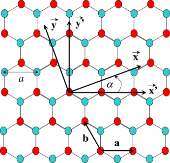
Figure 1: (Color online) Schematic representation of the graphene lattice and two useful reference frames. Here $\alpha$ is the CNT chiral angle. The $y$ axis is parallel to the nanotube axis, whereas the $x$ axis is parallel to the chiral vector.

The CNT is a cylinder of radius

$$R=\frac{L}{2\pi}=\frac{a}{2\pi}\sqrt{n^{2}_{a}+n^{2}_{b}-n_{a}n_{b}},$$ (6)

and axis parallel to ${\bf{T}}$. It is natural to use cylindrical coordinates, ${\bf{r}}=\left(\rho,\theta,y\right)$, where $\rho\in[0,\infty)$ is the distance from the nanotube axis, $\theta\in[0,2\pi)$ is the azimuthal angle, and $y\in(-\infty,+\infty)$ is the axial coordinate. A vector lying in the original 2D graphene plane, ${\bf{r}}=x\overrightarrow{\bf{x}}+y\overrightarrow{\bf{y}}$, is now described by coordinates $\rho=R$, $\theta=(x/R)\mod(2\pi)$, and $y$. The origin of the reference frame is chosen such that atom ${\bf{R}}_{\text{B}}(0,0)$ in Eq. (1) has coordinates $(\rho,\theta,y)=(R,0,0)$. The cylindrical coordinates obtained from (1) are given by

$$\theta_{\text{A}}(n_{1},n_{2})=\pi\!\left[\frac{n_{a}\left(2n_{1}\!-\!n_{2}\right)-n_{b}\left(n_{1}\!-\!2n_{2}\!-\!1\right)}{n^{2}_{a}+n^{2}_{b}-n_{a}n_{b}}\!\!\!\!\!\mod 2\right],$$

$$y_{\text{A}}(n_{1},n_{2})=a\frac{\sqrt{3}}{2}\frac{n_{a}\left(n_{2}+\frac{2}{3}\right)-n_{b}\left(n_{1}+\frac{1}{3}\right)}{\sqrt{n^{2}_{a}+n^{2}_{b}-n_{a}n_{b}}},$$

$$\theta_{\text{B}}(n_{1},n_{2})=\pi\!\left[\frac{n_{a}\left(2n_{1}-n_{2}\right)-n_{b}\left(n_{1}-2n_{2}\right)}{n^{2}_{a}+n^{2}_{b}-n_{a}n_{b}}\!\!\!\!\!\mod 2\right],$$

$$y_{\text{B}}(n_{1},n_{2})=a\frac{\sqrt{3}}{2}\frac{n_{a}n_{2}-n_{b}n_{1}}{\sqrt{n^{2}_{a}+n^{2}_{b}-n_{a}n_{b}}}.$$ (7)

The set of equations (7) maps the atomic positions of the original graphene plane into the locations of atoms on the CNT surface by letting $n_{1}$ and $n_{2}$ vary in $\mathbb{Z}$. A drawback is that there is an infinite number of atoms that are mapped into the same position on the CNT surface, i.e., those atoms with the same values of $y$ and $(x/R)\mod(2\pi)$. Since we will need to avoid multiple countings of atoms, it is more convenient to express atomic positions as a function of the two indexes $(n,j)$, unrelated to the original graphene geometry, defined as follows: $n$ fixes the axial coordinate and $j$ labels atoms lying on the same cross section of the CNT, given by $n$. The resulting expressions are

$$y_{\text{B}}(n)=\frac{\sqrt{3}a}{2\sqrt{\nu_{a}^{2}+\nu_{b}^{2}-\nu_{a}\nu_{b}}}n,$$

$$\theta_{\text{B}}(n,j)=\left\{\left[n\theta_{\text{B}}(1)\right]\mod\left(\frac{2\pi}{f_{ab}}\right)\right\}+j\frac{2\pi}{f_{ab}},$$

$$y_{\text{A}}(n)=y_{\text{B}}(n)+\Delta y_{\text{AB}},$$

$$\theta_{\text{A}}(n,j)=\left\{\left[n\theta_{\text{B}}(1)+\Delta\theta_{\text{AB}}\right]\mod\left(\frac{2\pi}{f_{ab}}\right)\right\}+j\frac{2\pi}{f_{ab}},$$ (8)

with $n\in\mathbb{Z}$ for a tube of indefinite length, $j\in\{0,1,\ldots,f_{ab}-1\}$, $f_{ab}=\text{GCD}\{n_{a},n_{b}\}$, with $n_{a}=f_{ab}\nu_{a}$ and $n_{b}=f_{ab}\nu_{b}$ so that integers $\nu_{a}$ and $\nu_{b}$ are coprime (if $n_{b}=0$ then $f_{ab}=n_{a}$, $\nu_{a}=1$, and $\nu_{b}=0$), $\theta_{\text{B}}(1)$ is an angular offset depending on $n_{a}$ and $n_{b}$, whose expression is given in App. A [Eq. (103)], and

$$\Delta y_{\text{AB}}=\frac{\sqrt{3}a}{2\sqrt{\nu_{a}^{2}+\nu_{b}^{2}-\nu_{a}\nu_{b}}}\frac{1}{3}\Big{(}2\nu_{a}-\nu_{b}\Big{)},$$

$$\Delta\theta_{\text{AB}}=\frac{\nu_{b}\pi}{f_{ab}(\nu_{a}^{2}+\nu_{b}^{2}-\nu_{a}\nu_{b})}.$$ (9)

Equations (8), (9), and (103) allow to uniquely determine the cylindrical coordinates of the atoms a nanotube of arbitrary chirality. Appendix A provides the details of the derivation of Eqs. (8) and (9) starting from Eq. (7).

III Many-body Hamiltonian

The many-body Hamiltonian, $\hat{H}=\hat{H}_{\text{SP}}+\hat{V}$, is the sum of two terms. The first one, $\hat{H}_{\text{SP}}$, is the single-particle Hamiltonian (121) of a quantum dot embedded in a semiconducting CNT, which includes kinetic energy, confinement potential, and spin-orbit coupling (see Appendix B for full details). The second one, $\hat{V}$, is the Coulomb interaction potential.

We consider a gate-defined QD, whose confinement potential is a soft harmonic trap of electrostatic origin:Kumar90 ; Reimann02

$$V_{\text{QD}}(y)=\frac{1}{2}m^{*}\omega_{0}^{2}y^{2},$$ (10)

with $m^{*}$ being the effective mass and $\omega_{0}$ the characteristic harmonic oscillator frequency. The QD size in real space is given by the characteristic length $\ell_{\text{QD}}=\sqrt{\hbar/(m^{*}\omega_{0})}$. The Hamiltonian $\hat{H}_{\text{SP}}$ is  written on the basis of the single-particle eigenstates as:

$$\hat{H}_{\text{SP}}=\sum_{n}\sum_{\tau}\sum_{\sigma}\varepsilon_{n\tau\sigma}\hat{c}^{\dagger}_{n\tau\sigma}\hat{c}_{n\tau\sigma},$$ (11)

where $\hat{c}_{n\tau\sigma}$ destroys a fermion occupying the $n$th harmonic-oscillator excited state with spin $\sigma$, isospin $\tau$, and energy $\varepsilon_{n\tau\sigma}$ given by Eq. (127).

The Coulomb potential $\hat{V}$, which scatters different states $\{n,\tau,\sigma\}$, is made of two terms,Secchi09 ; Secchi10

$$\hat{V}=\hat{V}_{\text{FW}}+\hat{V}_{\text{BW}},$$ (12)

respectively for forward

$$\hat{V}_{\text{FW}}=\frac{1}{2}\sum_{abcd}\sum_{\tau\tau^{\prime}}\sum_{\sigma\sigma^{\prime}}V_{a,b;c,d}^{(\text{FW})}\hat{c}^{\dagger}_{a\tau\sigma}\hat{c}^{\dagger}_{b\tau^{\prime}\sigma^{\prime}}\hat{c}_{c\tau^{\prime}\sigma^{\prime}}\hat{c}_{d\tau\sigma}$$ (13)

and backward scattering

$$\hat{V}_{\text{BW}}=\frac{1}{2}\sum_{abcd}\sum_{\tau}\sum_{\sigma\sigma^{\prime}}V_{a,b;c,d}^{(\text{BW})}(\tau)\hat{c}^{\dagger}_{a\tau\sigma}\hat{c}^{\dagger}_{b-\tau\sigma^{\prime}}\hat{c}_{c\tau\sigma^{\prime}}\hat{c}_{d-\tau\sigma}.$$ (14)

Note that the FW term scatters different orbital states while conserving the individual isospins of the interacting electrons, whereas the BW term also exchanges the (opposite) isospins of the interacting electrons. There is no BW term for electrons with like isospins. The quantities $V_{a,b;c,d}^{(\text{FW})}$ and $V_{a,b;c,d}^{(\text{BW})}(\tau)$, appearing respectively in Eqs. (13) and (14), are the two-body matrix elements of Coulomb interaction. We refer the reader to Ref. Secchi10, for a detailed discussion of the FW term and focus on the BW term in the following.

IV Backward scattering

This section is devoted to the analysis of the BW scattering term. The starting point is our previous treatment of the BW potential as a contact force, as reported in Ref. Secchi10, . Here we extend our theory to include the effect of the CNT curvature.

IV.1 Backward scattering for the curved tube geometry

We recall from Ref. Secchi10, [Eq. (B5)] the generic expression of the two-body BW scattering matrix element that appears in the operator (14),

$$V^{(\text{BW})}_{a,b;c,d}(\tau)\!=\!\frac{L_{y}^{2}}{4N_{c}^{2}}\ell_{\text{QD}}^{-2}\sum_{p,p^{\prime}}\text{e}^{\text{i}\tau\phi_{pp^{\prime}}}\!\!\sum_{\underline{R}_{p}}\!\sum_{\underline{R}^{\prime}_{p^{\prime}}}\text{e}^{\text{i}\tau\left(\underline{M}^{\prime}-\underline{M}\right)\cdot\left(\underline{R}_{p}-\underline{R}^{\prime}_{p^{\prime}}\right)}$$

$$\quad\times U\left(\left|\underline{R}_{p}-\underline{R}^{\prime}_{p^{\prime}}\right|\right)F^{*}_{a}(y_{p})F^{*}_{b}(y^{\prime}_{p^{\prime}})F_{c}(y^{\prime}_{p^{\prime}})F_{d}(y_{p}),$$ (15)

where $p,p^{\prime}\in\{\text{A},\text{B}\}$ are the sublattice indexes, $\phi_{\text{AA}}=\phi_{\text{BB}}=0$, $\phi_{\text{AB}}=-\phi_{\text{BA}}=2\alpha+\frac{2\pi}{3}$, $\underline{M}$ and $\underline{M}^{\prime}$ are the wave vectors of the conduction-band minima in the two valleys, $\underline{R}_{p}$ is the position of an atom of the $p$ sublattice, $U$ is the interaction potential, $N_{c}$ is the number of sublattice sites, $L_{y}$ is the CNT length, and $F_{n}$ is the envelope function of the $n$th harmonic-oscillator state (see also Appendix B). With respect to Eq. (B5) of Ref. Secchi10, here we have used cylindrical coordinates and included a minus sign into phases $\phi_{\text{AB}}$. Equation (15) is derived exploiting the localization of the $2p_{z}$ orbitals close to the atomic nuclei, whereas the envelope function $F_{n}(y)$ varies on the longer length scale $\ell_{\text{QD}}$, hence we assume $\left|\phi_{2p_{z}}({\bf{r}}-{\bf{R}}_{p})\right|^{2}\approx\delta({\bf{r}}-{\bf{R}}_{p})\mathcal{V}_{\text{CNT}}$. Since this approximation washes out all effects related to the atomic orbitals, as an improvement we replace in Eq. (15) the Coulomb potential with the Ohno potential,Ohno64 ; Ando06 ; Mayrhofer08

$$U({\bf{r}}-{\bf{r}}^{\prime})=U_{0}\left[1+\epsilon^{2}\left|{\bf{r}}-{\bf{r}}^{\prime}\right|^{2}U_{0}^{2}/e^{4}\right]^{-1/2},$$ (16)

which at short distances tends to the Hubbard-like value of the Coulomb repulsion between two electrons sitting on the $2p_{z}$ orbital, $U_{0}\approx 15$ eV, whereas at long distances evolves into the screened Coulomb potential with static dielectric constant $\epsilon$.

By making explicit the dependence of the atomic positions on the indexes $(n,j)$ as illustrated in Sec. II, we write the interaction potential in cylindrical coordinates in the following symbolic form:

$$U\left[\left|\underline{R}_{p}(n,j)-\underline{R}^{\prime}_{p^{\prime}}(n^{\prime},j^{\prime})\right|\right]$$

$$\equiv U\left\{\left[y_{p}(n)-y_{p^{\prime}}(n^{\prime})\right]^{2},\sin^{2}\left[\frac{\theta_{p}(n,j)-\theta_{p^{\prime}}(n^{\prime},j^{\prime})}{2}\right]\right\}.$$ (17)

After a lengthy calculation that is detailed in Appendix C, the matrix element (15) is transformed into

$$V^{(\text{BW})}_{a,b;c,d}(\tau)=\frac{\sqrt{3}a^{2}}{16\pi R}\ell_{\text{QD}}^{-2}\int_{-\infty}^{+\infty}\text{d}y\sum_{n\in\mathbb{Z}}\Big{\{}$$

$$2f_{\tau}(n)F^{*}_{a}[y+y_{\text{B}}(n)]F^{*}_{b}(y)F_{c}(y)F_{d}[y+y_{\text{B}}(n)]$$

$$+g_{\tau}(n)F^{*}_{a}[y+y_{\text{A}}(n)]F^{*}_{b}(y)F_{c}(y)F_{d}[y+y_{\text{A}}(n)]$$

$$+g_{-\tau}(n)F^{*}_{a}(y)F^{*}_{b}[y+y_{\text{A}}(n)]F_{c}[y+y_{\text{A}}(n)]F_{d}(y)\Big{\}},$$ (18)

where we have introduced two characteristic functions,

$$f_{\tau}(n)\equiv\text{e}^{\text{i}\tau\Delta M_{k}\cdot y_{\text{B}}(n)}\sum_{j=0}^{f_{ab}-1}\text{e}^{\text{i}\tau\Delta M_{\kappa}\cdot\theta_{\text{B}}(n,j)}U_{\text{B}}(n,j),$$

$$g_{\tau}(n)\equiv\text{e}^{\text{i}\tau\phi_{\text{AB}}}\text{e}^{\text{i}\tau\Delta M_{k}\cdot y_{\text{A}}(n)}\sum_{j=0}^{f_{ab}-1}\text{e}^{\text{i}\tau\Delta M_{\kappa}\cdot\theta_{\text{A}}(n,j)}U_{\text{A}}(n,j),$$ (19)

with

$$(\Delta M_{k},\Delta M_{\kappa})\equiv(M^{\prime}_{k}-M_{k},M^{\prime}_{\kappa}-M_{\kappa}),$$ (20)

and

$$U_{p}(n,j)\equiv U\left\{\left[y_{p}(n)\right]^{2},\sin^{2}\left[\frac{\theta_{p}(n,j)}{2}\right]\right\}$$ (21)

for $p\in\{\text{A, B}\}$.

The characteristic functions $f_{\tau}(n)$ and $g_{\tau}(n)$ determine the length scale and strength of BW interaction. In order to understand their physical meaning, we inspect the expression (18) of the matrix element for BW scattering. The function $f_{\tau}(n)$ [$g_{\tau}(n)$] is weighted by the envelope functions of the interacting electrons, evaluated in positions along the CNT axis which are separated by $y_{\text{B}}(n)$ [$y_{\text{A}}(n)$]. Recalling the expressions (8) of the axial coordinates, we see that two coordinates differing by $y_{\text{B}}(n)$ belong to the same sublattice, while two coordinates differing by $y_{\text{A}}(n)$ belong to different sublattices. Therefore, the functions $f_{\tau}(n)$ and $g_{\tau}(n)$ measure the strength, respectively, of the intra- and inter-sublattice contributions to BW scattering. Moreover, since the distance between $y$ and $y+y_{\text{B(A)}}(n)$ is linear with $\left|n\right|$ and BW interaction is short-ranged, we expect $f_{\tau}(n)$ and $g_{\tau}(n)$ to vanish rapidly with increasing $\left|n\right|$, as further discussed in subsection IV.3. To gain a deeper insight into the properties of $f_{\tau}(n)$ and $g_{\tau}(n)$, it is convenient to work out the form of the BW scattering operator in first quantization, which is done in the following subsection.

IV.2 BW scattering potential in first quantization

In this subsection we explicitly state the form of the BW scattering operator in the coordinate space representation.

Let us introduce the isospinor $\varphi_{\tau}(t)$, which depends on the coordinate $t=\pm 1$ and is eigenstate of the isospin operator $\hat{\tau}$, with $\hat{\tau}(t)\varphi_{\tau}(t)=\tau\varphi_{\tau}(t)$. The electron has three coordinates: position along the axis $y$, spin $s$, and isospin $t$, indicated as a whole by $\bm{z}\equiv(y,s,t)$. The wave function $\Psi_{n\sigma\tau}(\bm{z})$ is factorized as

$$\Psi_{n\sigma\tau}(\bm{z})=\left[\ell_{\text{QD}}^{-1/2}F_{n}(y)\right]\otimes\chi_{\sigma}(s)\otimes\varphi_{\tau}(t),$$ (22)

with the normalizations

$$\ell_{\text{QD}}^{-1}\int\text{d}y\;F^{*}_{n}(y)F_{n^{\prime}}(y)=\delta_{nn^{\prime}},$$

$$\sum_{s}\chi^{*}_{\sigma}(s)\chi_{\sigma^{\prime}}(s)=\delta_{\sigma\sigma^{\prime}},$$

$$\sum_{t}\varphi^{*}_{\tau}(t)\varphi_{\tau^{\prime}}(t)=\delta_{\tau\tau^{\prime}}.$$ (23)

As a straightforward generalization, the $N$-electron wave function, $\Psi(\bm{z}_{1},\bm{z}_{2},\ldots,\bm{z}_{N})$, depends on the set of orbital, $(y_{1},y_{2},\ldots,y_{N})$, spin, $(s_{1},s_{2},\ldots,s_{N})$, and isospin coordinates, $(t_{1},t_{2},\ldots,t_{N})$.

We look for the explicit expression of the BW scattering potential acting on $\bm{z}$ coordinates. It is easy to check that this must be a two-body potential of the form $\hat{V}_{\text{BW}}(y,t;y^{\prime},t^{\prime})$, acting on the orbital and isospin coordinates but not on spins. This is obtained by rewriting the second-quantized expression (14) with the help of the isospinor formalism. In fact, the field annihilation operator is

$$\hat{\Psi}(\bm{z})\equiv\sum_{n}\sum_{\sigma}\sum_{\tau}\hat{\Psi}_{n\sigma\tau}(\bm{z}),$$ (24)

with

$$\hat{\Psi}_{n\sigma\tau}(\bm{z})\equiv\Psi_{n\sigma\tau}(\bm{z})\hat{c}_{n\sigma\tau}.$$ (25)

The BW term of the Hamiltonian is written in terms of the operator $\hat{V}_{\text{BW}}(\bm{z};\bm{z}^{\prime})\equiv\hat{V}_{\text{BW}}(y,t;y^{\prime},t^{\prime})$ as

$$\hat{V}_{\text{BW}}=\frac{1}{2}\int\text{d}\bm{z}\int\text{d}\bm{z}^{\prime}\hat{\Psi}^{\dagger}(\bm{z})\hat{\Psi}^{\dagger}(\bm{z}^{\prime})\hat{V}_{\text{BW}}(\bm{z};\bm{z}^{\prime})\hat{\Psi}(\bm{z}^{\prime})\hat{\Psi}(\bm{z}),$$ (26)

where $\int\text{d}\bm{z}\equiv\int\text{d}y\sum_{s}\sum_{t}$ and we mix operator symbols of first- and second-quantization. After substituting the expansion (24) into (26), the result must be equal to (14). By further imposing the symmetry of the BW potential under coordinate permutation, $\hat{V}_{\text{BW}}(y,t;y^{\prime},t^{\prime})=\hat{V}_{\text{BW}}(y^{\prime},t^{\prime};y,t)$, we obtain

$$\hat{V}_{\text{BW}}(y,t;y^{\prime},t^{\prime}) =W_{\text{BW}}(y,y^{\prime})\hat{\tau}^{+}(t)\hat{\tau}^{-}(t^{\prime})$$

$$+W_{\text{BW}}(y^{\prime},y)\hat{\tau}^{-}(t)\hat{\tau}^{+}(t^{\prime}),$$ (27)

where $W_{\text{BW}}(y,y^{\prime})$ is an operator acting on the orbital coordinates only, given by

$$W_{\text{BW}}(y,y^{\prime})=\!\sum_{n\in\mathbb{Z}}\!\Big{\{}\left[f_{+1}(n)+f_{-1}(-n)\right]\delta\!\left[y^{\prime}-y+y_{\text{B}}(n)\right]$$

$$+g_{+1}(n)\delta\!\left[y^{\prime}-y+y_{\text{A}}(n)\right]+g_{-1}(n)\delta\!\left[y^{\prime}-y-y_{\text{A}}(n)\right]\Big{\}}$$

$$\times\frac{\sqrt{3}a^{2}}{16\pi R},$$ (28)

and we have introduced the ladder operators of isospin:

$$\begin{array}[]{ll}\hat{\tau}^{+}(t)\varphi_{-1}(t)=\varphi_{+1}(t),&\hat{\tau}^{+}(t)\varphi_{+1}(t)=0,\\ \hat{\tau}^{-}(t)\varphi_{-1}(t)=0,&\hat{\tau}^{-}(t)\varphi_{+1}(t)=\varphi_{-1}(t).\end{array}$$ (31)

These operators induce transitions between different conduction-band valleys as an effect of Coulomb interaction, exchanging the crystal momentum of electrons. We will see a similar effect with short-range disorder, which acts as a crystal momentum scatterer randomly placed in the CNT.

IV.3 Properties of functions $f$ and $g$

In this subsection we discuss the properties of the characteristic functions $f_{\tau}(n)$ and $g_{\tau}(n)$, especially relevant as their real parts determine the fine structure of two-electron energy levels (cf. Sec. V). We consider $\Re[f_{+1}]=\Re[f_{-1}]\equiv\Re[f]$ and $\Re[g_{+1}]=\Re[g_{-1}]\equiv\Re[g]$ for a few representative tube geometries. Throughout the section we fix the dielectric constant as $\epsilon=3.5$.

Equation (19) shows that $f$ ($g$) depends on the arrangement of the atoms in the B (A) sublattice. For semiconducting nanotubes, an examplar case is the zigzag configuration, with either $\alpha=0$ ($n_{b}=0$) or $\alpha=\pi/3$ ($n_{a}=n_{b}$). In this case $f$ as a function of the axial coordinate $y$ ($n$) is even with respect to the origin (Figs. 2 and 3), whereas the function $g$ does not have a definite symmetry, as shown in Figs. 4 and 5. Indeed, the A sublattice is asymmetric with respect to $y=0$: for example, if $n_{b}=0$, then for any $n_{a}$ we have $T=\sqrt{3}a$ and $\Delta y_{\text{AB}}=a/\sqrt{3}=T/3$, so the A axial coordinates most close to $0$ are respectively $y_{\text{A}}(0)=T/3$ and $y_{\text{A}}(-1)=-T/6$. The zigzag configuration also maximizes the number of atoms on each allowed cross section and, conversely, minimizes the density of allowed $y$ coordinates along the tube axis. On the other hand, for generic chiral tubes there are more allowed axial coordinates with fewer atoms contributing to the circumferential cross section. Since in those cases even the arrangement of B atoms is not symmetric around $y=0$, neither $f$ nor $g$ exhibit a well-defined symmetry.

Figure 2(a) shows $\Re[f]$ for the achiral ($\alpha=0$) zigzag tube $(n_{a},n_{b})=(92,0)$ (black bullets) and chiral tube $(n_{a},n_{b})=(91,1)$ (red curve) obtained by applying a small twist $(-1,1)$ to the zigzag one. The tube radius $R$ is approximately the same ($\approx 3.6$ nm) in both cases but the variation of the atom arrangement along the axis causes an appreciable variation of the profile of $f(n)$. In addition to the dominant maximum in the origin, $\Re[f]$ of the chiral tube exhibits many oscillations on the length scale of $a/100$, whereas the profile of the zigzag tube is smoother because only a few axial coordinates are allowed. Nevertheless, for such a large radius, the oscillations of $\Re[f]$ of the chiral tube are reminescent of those of the zigzag tube as the positions of the highest maxima overlap. For a smaller radius, the symmetry-breaking effect of a $(-1,1)$ twist of the zigzag tube is larger, as seen in Fig. 2(b) for the tube $(n_{a},n_{b})=(20,0)$. Apart from the central peak, the profiles of the chiral and zigzag tubes now deviate more significantly than in Fig. 2(a). Note that $\Re[f]$ with $\alpha=0$ depends very weakly on the radius $R$ (i.e., $n_{a}$).

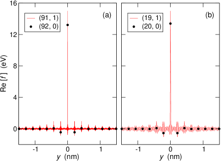
Figure 2: (Color online) $\Re[f]$ vs axial coordinate $y$, for CNTs with chiral angle close to $\alpha=0$. (a) Tubes with a large radius: zigzag CNT with $(n_{a},n_{b})=(92,0)$ and $R=3.602$ nm (black bullets) and chiral tube with $(n_{a},n_{b})=(91,1)$ and $R=3.543$ nm (red curve). (b) Tubes with a smaller radius: zigzag CNT with $(n_{a},n_{b})=(20,0)$ and $R=0.783$ nm (black bullets) and chiral tube with $(n_{a},n_{b})=(19,1)$ and $R=0.725$ nm (red curve). Lines are guides to the eye. The parameters are $\epsilon=3.5$ and $U_{0}=15$ eV.

Results for $\alpha=\pi/3$ zigzag tubes with $n_{a}=n_{b}$ are shown in Fig. 3 (black bullets) for different radii ($R\approx$ 1.8 and 0.4 nm respectively in panels a and b), together with data for tubes obtained by applying a $(1,-1)$ twist (red curves). Although the CNTs with $\alpha=0$ and $\alpha=\pi/3$ are equivalent, the functions plotted in Fig. 3 differ from those for $\alpha=0$ because the arrangement of the atoms is shifted with respect to $y=0$ in the two cases. This shows that $f$ depends strongly on the chiral angle. On the other hand, the comparison between chiral and achiral tubes exhibits the same features as in Fig. 2.

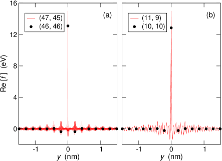
Figure 3: (Color online) $\Re[f]$ vs axial coordinate $y$, for CNTs with chiral angle close to $\alpha=\pi/3$. (a) Tubes with a large radius: zigzag CNT with $(n_{a},n_{b})=(46,46)$ and $R=1.801$ nm (black bullets) and chiral tube with $(n_{a},n_{b})=(47,45)$ and $R=1.802$ nm (red curve). (b) Tubes with a smaller radius: zigzag CNT with $(n_{a},n_{b})=(10,10)$ and $R=0.392$ nm (black bullets) and chiral tube with $(n_{a},n_{b})=(11,9)$ and $R=0.397$ nm (red curve). Lines are guides to the eye. The parameters are $\epsilon=3.5$ and $U_{0}=15$ eV.

In Figs. 4 and 5 we plot $\Re[g]$ for the eight nanotubes considered before. The $g$ function, which provides the scattering between sublattices A and B, gives generically a weaker contribution to the BW Hamiltonian than the $f$ function, which induces scattering within the same sublattice. This may be seen by the difference between the maximum values of $\Re[f]$ (Figs. 2 and 3) and $\Re[g]$ (Figs. 4 and 5). Inspection of figures Figs. 4 and 5 also reveals that the $g$ function for $\alpha=0$ or $\alpha=\pi/3$ depends very weakly on $R$ and that small distortions with respect to the zigzag configuration are sufficient to change significantly the profiles of $g(n)$, similarly to the features of function $f$.

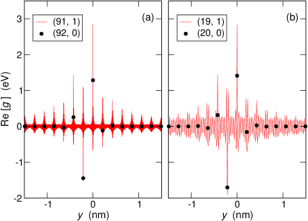
Figure 4: (Color online) $\Re[g]$ vs axial coordinate $y$, for CNTs with chiral angle close to $\alpha=0$. The tubes are the same as those studied in Fig. 2.

Figure 5: (Color online) $\Re[g]$ vs axial coordinate $y$, for CNTs with chiral angle close to $\alpha=\pi/3$. The tubes are the same as those studied in Fig. 3.

The plots of $f$ and $g$ provide an insight into the features of BW scattering. Both $f(n)$ and $g(n)$ are significantly different from zero only close to $n=0$, which confirms the short-range nature of BW interaction.Ando06 From Eq. (28) it is clear that the dominant contribution comes from values of $f(n)$ close to $n=0$, with $f(0)$ being of the order of the Hubbard parameter $U_{0}$. Function $g(n)$ has a nearly-zero average on a length scale of few nanometers (see Figs. 4 and 5), over which the QD envelope functions are not expected to vary appreciably, therefore its contribution is much smaller than that of $f$. Therefore, a first approximation is $f(n)\approx U_{0}\delta_{n0}$ and $g(n)\approx 0$, which, applied to (28), gives the approximated form of BW potential appearing in Eq. (27):

$$\hat{V}^{(0)}_{\text{BW}}(y,t;y^{\prime},t^{\prime}) \approx U_{0}\frac{\sqrt{3}a^{2}}{8\pi R}\delta(y-y^{\prime})$$

$$\times\left[\hat{\tau}^{+}(t)\hat{\tau}^{-}(t^{\prime})+\hat{\tau}^{-}(t)\hat{\tau}^{+}(t^{\prime})\right].$$ (32)

This form reproduces the results of Refs. Ando06, ; Secchi09, ; Secchi10, , showing that the BW scattering is expected to act significantly only on those many-body states in which electrons have a non-zero probability of being in contact. We study in detail the two-electron system in the next section.

V Two electrons in a carbon-nanotube quantum dot

In this section we recall from our previous studiesSecchi09 ; Secchi10 ; Pecker13 the main features of the two-electron system in the absence of BW scattering. The effect of the BW interaction potential will be analyzed in the next section.

The envelope-function Hamiltonian of two interacting electrons in a CNT QD is

$$\hat{H}(\bm{z}_{1},\bm{z}_{2}) =K\left(\partial^{2}_{y_{1}},\partial^{2}_{y_{2}}\right)+V_{\text{QD}}\left(y_{1},y_{2}\right)+V_{\text{FW}}\left(\left|y_{1}-y_{2}\right|\right)$$

$$+\hat{V}_{\text{BW}}\left(y_{1},t_{1};y_{2},t_{2}\right)+\hat{H}_{\text{SO}}\left(s_{1},t_{1};s_{2},t_{2}\right),$$ (33)

where we have put the hat symbol only on the operators acting on spins and isospins. Here $K$ is the kinetic energy, $V_{\text{QD}}$ is the QD confinement potential, $V_{\text{FW}}$ is the FW scattering interaction (acting on orbital coordinates only), $\hat{V}_{\text{BW}}$ is the BW scattering interaction, and $\hat{H}_{\text{SO}}$ is the SO interaction,

$$\hat{H}_{\text{SO}}\left(s_{1},s_{2};t_{1},t_{2}\right)=\nu\Delta_{\text{SO}}\frac{\gamma}{R}\left[\hat{\sigma}(s_{1})\hat{\tau}(t_{1})+\hat{\sigma}(s_{2})\hat{\tau}(t_{2})\right].$$ (34)

We set

$$\hat{H}\equiv H_{0}+\hat{H}^{\prime},$$

$$H_{0}\equiv K+V_{\text{QD}}+V_{\text{FW}},$$

$$\hat{H}^{\prime}\equiv\hat{V}_{\text{BW}}+\hat{H}_{\text{SO}},$$ (35)

assuming that $\hat{H}^{\prime}$ can be treated as a small perturbation of $H_{0}$, as confirmed a posteriori by numerical evidence.Secchi09 ; Secchi10 The eigenvalue equation for $H_{0}$ is

$$H_{0}\Psi_{k,j}(\bm{z}_{1},\bm{z}_{2})=E_{0}(k)\Psi_{k,j}(\bm{z}_{1},\bm{z}_{2}),$$ (36)

where the wave function may be factorized as

$$\Psi_{k,j}(\bm{z}_{1},\bm{z}_{2})=\ell_{\text{QD}}^{-1}\psi_{k}(y_{1},y_{2})\otimes\xi_{j}(s_{1},t_{1};s_{2},t_{2}),$$ (37)

with $\psi_{k}(y_{1},y_{2})$ being the orbital component and $\xi_{j}(s_{1},t_{1};s_{2},t_{2})$ the spin-valley component of the wave function. They are normalized as

$$\ell_{\text{QD}}^{-2}\int\!\!\text{d}y_{1}\!\!\!\int\!\!\text{d}y_{2}\,\psi^{*}_{k}(y_{1},y_{2})\psi_{k^{\prime}}(y_{1},y_{2})=\delta_{kk^{\prime}},$$

$$\sum_{s_{1},s_{2}}\sum_{t_{1},t_{2}}\xi_{j}^{*}(s_{1},t_{1};s_{2},t_{2})\xi_{j^{\prime}}(s_{1},t_{1};s_{2},t_{2})$$

$$\quad=\delta_{jj^{\prime}}.$$ (38)

The factorization (37) is always possible for two electrons, hence both orbital and spin-valley wave functions have a definite symmetry under coordinate permutation while the total product $\Psi_{k,j}(\bm{z}_{1},\bm{z}_{2})$ is antisymmetric. It follows that the orbital and spin-valley parts are one even and the other one odd under particle exchange. Since $H_{0}$ does not act on spin and isospin coordinates, the energy $E_{0}(k)$ depends only on the orbital component and is possibly degenerate with respect to different spin-valley projections. The complete set of spin-valley functions for two electrons consists of six antisymmetric and ten symmetric components.Secchi09 ; Pecker13 For example, the six antisymmetric spin-valley functions are obtained by multiplying either a spin singlet times an isospin triplet or a spin triplet times an isospin singlet (see also Tables 1 and 2). Therefore (in the absence of orbital degeneracy) $E_{0}(k)$ is either six-fold or ten-fold degenerate when $\psi_{k}$ is respectively even or odd under coordinate exchange.Secchi09 ; Secchi10 ; Pecker13

We next discuss the features of the spectrum $E_{0}(k)$ in the case of harmonic confinement,

$$V_{\text{QD}}(y_{1},y_{2})=\frac{1}{2}m^{*}\omega_{0}^{2}\left(y_{1}^{2}+y_{2}^{2}\right).$$ (39)

Since the QD potential is quadratic and the interaction potential $V_{\text{FW}}$ depends on $\left|y_{1}-y_{2}\right|$ only, the canonical transformation to (normalized) center-of-mass (CM) and relative-motion (RM) coordinates

$$y_{\text{CM}}=\frac{y_{1}+y_{2}}{\sqrt{2}},\quad y_{\text{RM}}=\frac{y_{1}-y_{2}}{\sqrt{2}}$$ (40)

allows to separate the Hamiltonian $H_{0}$ into the sum of two terms,

$$H_{0}\equiv H_{\text{CM}}+H_{\text{RM}},$$

$$H_{\text{CM}}\equiv-\frac{\hbar^{2}}{2m^{*}}\frac{\partial^{2}}{\partial y^{2}_{\text{CM}}}+\frac{1}{2}m^{*}\omega_{0}^{2}y^{2}_{\text{CM}},$$

$$H_{\text{RM}}\equiv-\frac{\hbar^{2}}{2m^{*}}\frac{\partial^{2}}{\partial y^{2}_{\text{RM}}}+\frac{1}{2}m^{*}\omega_{0}^{2}y^{2}_{\text{RM}}+V_{\text{FW}}\left(\sqrt{2}\left|y_{\text{RM}}\right|\right),$$ (41)

which depend separately on the coordinates $y_{\text{CM}}$ and $y_{\text{RM}}$. We may factorize the orbital wave function $\psi(y_{1},y_{2})\rightarrow\psi(y_{\text{CM}},y_{\text{RM}})$ as

$$\psi_{n_{\text{CM}},m}(y_{\text{CM}},y_{\text{RM}})\equiv F_{n_{\text{CM}}}(y_{\text{CM}})\psi_{m}(y_{\text{RM}}),$$ (42)

where the CM wave function is determined by $H_{\text{CM}}$ and is an eigenstate of the harmonic oscillator,

$$F_{n}(y)=u_{n}({\ell^{-1}_{\text{QD}}y}),$$

$$u_{n}(Y)=\left(\pi 2^{n}n!\right)^{-1/2}\text{e}^{-Y^{2}/2}\mathcal{H}_{n}(Y),$$ (43)

with eigenvalue

$$E\left(n_{\text{CM}}\right)=\left(n_{\text{CM}}+\frac{1}{2}\right)\hbar\omega_{0},$$ (44)

for $n\in\{0,1,2,\ldots\}$ ($\mathcal{H}_{n}(Y)$ is the Hermite polynomial of order $n$). The problem associated with the RM wave function $\psi_{m}$ depends on the interaction and must be solved numerically. Since the CM wave function is symmetric under the interchange of $y_{1}$ and $y_{2}$, the symmetry of the total orbital wave function is the same as that of the RM wave function.

Figure 6 shows the low-energy spectrum $E_{0}(k)$ associated to the Hamiltonian $H_{0}$ appearing in (41), obtained from exact diagonalization,Rontani06 ; Secchi09 ; Secchi10 ; Secchi12 ; Pecker13 as a function of the confinement strength $\hbar\omega_{0}$. The dielectric constant $\epsilon=3.5$ and the CNT radius $R=1$ nm are typical values for Coulomb blockade experiments. The quantity on the vertical axis is the excitation energy, i.e., $E_{0}(k)-E_{0}(k=0)$, in units of $\hbar\omega_{0}$. This is ruled by the competition between the energy scales respectively associated to the confinement potential, $\hbar\omega_{0}$, and FW Coulomb interaction. When $\hbar\omega_{0}$ is small the system is in the strongly-interacting Wigner molecule regime Secchi09 ; Secchi10 ; Secchi12 ; Pecker13 whereas when $\hbar\omega_{0}$ is large Coulomb interaction is negligible and the non-interacting (NI) picture holds. Below we consider in some detail the two limit regimes.

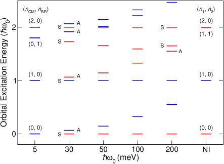
Figure 6: (Color online) Excitation energies of two electrons, in units of $\hbar\omega_{0}$, vs $\hbar\omega_{0}$ (NI labels the limit $\hbar\omega_{0}\rightarrow\infty$). Red (blue) levels point to states even (odd) under spatial reflection, $\{y_{1}\rightarrow-y_{1},y_{2}\rightarrow-y_{2}\}$, whereas labels S (A) point to the (anti)symmetry of the wave function orbital component under particle exchange, $\{y_{1}\rightarrow y_{2},y_{2}\rightarrow y_{1}\}$. The data are obtained from exact diagonalization, with $\epsilon=3.5$ and $R=1$ nm.

V.1 Non-interacting regime

The NI regime is naturally described in the independent-particle framework. Orbital states are obtained as symmetrized or antisymmetrized products of single-particle orbitals $F_{n}(y)$ [Eq. (43)]. The quantum numbers $n_{1}$ and $n_{2}$ of the two orbitals occupied identify the excited states whose wave functions are

$$\psi_{\{n_{1},n_{1}\}}=F_{n_{1}}(y_{1})F_{n_{1}}(y_{2}),$$ (45)

if $n_{1}=n_{2}$, and

$$\psi_{\{n_{1},n_{2}\}}^{\pm}=\frac{1}{\sqrt{2}}\left[F_{n_{1}}(y_{1})F_{n_{2}}(y_{2})\pm F_{n_{2}}(y_{1})F_{n_{1}}(y_{2})\right]$$ (46)

if $n_{1}\neq n_{2}$, with excitation energies given by

$$E^{*}(n_{1},n_{2})=\left(n_{1}+n_{2}\right)\hbar\omega_{0}.$$ (47)

This picture, of course, may be recovered by alternatively using CM and RM coordinates. Expressions (45) and (46) show that states with $n_{1}\neq n_{2}$ produce two orthogonal orbital wave functions $\psi_{\{n_{1},n_{2}\}}^{\pm}$, respectively symmetric $(+)$ and antisymmetric $(-)$ under particle exchange, whereas if $n_{1}=n_{2}$ only the symmetric function is allowed (cf. Fig. 6). Therefore, a couple $(n_{1},n_{2})$ with $n_{1}\neq n_{2}$ specifies a set of sixteen states, obtained by summing the ten-fold degenerate A states with the six-fold degenerate S states, while if $n_{1}=n_{2}$ there are only six S states. Since energies depend on $(n_{1}+n_{2})$, we see that, e.g., the sets $(n_{1},n_{2})=(2,0)$ and $(n_{1},n_{2})=(1,1)$ are degenerate, with total degeneracy twenty-two. Note that states belonging to a same shell have all the same orbital parity, equal to $(-1)^{n_{1}+n_{2}}$, as seen in the NI column of Fig. 6.

V.2 Wigner molecule

The limit opposite to the NI regime is that of strong Coulomb repulsion. The low-energy states are then understood in terms of a Wigner molecule made of electrons localized in space, arranged in the geometrical configuration that minimizes the Coulomb repulsion in the presence of the confinement potential.Secchi09 ; Secchi10 ; Secchi12 ; Pecker13 The competition between Coulomb potential and quantum confinement tunes the classical equilibrium positions of the two electrons, $\pm\Lambda$, where

$$\Lambda=\left(\frac{e^{2}}{4\epsilon\omega_{0}^{2}m^{*}}\right)^{1/3}$$ (48)

is located at the maximum of the particle density along the axis. Indeed, the density weight is concentrated in Gaussians centered at $\pm\Lambda$, whose finite widths originate from the quantum fluctuations of the two electrons around their equilibrium positions. For a well-formed WM the Gaussian width is smaller than $\Lambda$, so the overlap between the localized electrons is small. In this limit, one may safely expand the dominant long-range part of Coulomb interaction, which goes like $\approx 1/\left(\epsilon\left|y_{1}-y_{2}\right|\right)$, around the equilibrium positions up to quadratic order.Secchi10

The approximated wave function is

$$\psi^{\pm}_{\{n_{\text{CM}},n_{\text{BR}}\}}=F_{n_{\text{CM}}}(y_{\text{CM}})\frac{3^{1/8}}{\sqrt{2}\mathcal{N}^{\pm}_{n_{\text{BR}}}}$$

$$\times\left\{F_{n_{\text{BR}}}[3^{1/4}(y_{\text{RM}}-\sqrt{2}\Lambda)]\pm F_{n_{\text{BR}}}[3^{1/4}(-y_{\text{RM}}-\sqrt{2}\Lambda)]\right\},$$ (49)

where the integer quantum number $n_{\text{BR}}$ counts the harmonic oscillation quanta of the antiphase normal mode known as breathing mode (BR). The BR characteristic frequency is $\sqrt{3}\omega_{0}$ and the total WM excitation energies are

$$E^{*}(n_{\text{CM}},n_{\text{BR}})=\left(n_{\text{CM}}+n_{\text{BR}}\sqrt{3}\right)\hbar\omega_{0},$$ (50)

as it may be checked in the $\hbar\omega_{0}=$ 5 meV column of Fig. 6. Symmetric $(+)$ and antisymmetric $(-)$ WM states with the same quantum numbers $(n_{\text{CM}},n_{\text{BR}})$ are sixteen-fold degenerate, since the overlap between localized electrons is negligible. This overlap enters Eq. (49) through the normalization constant $\mathcal{N}^{\pm}_{n_{\text{BR}}}$, which in turn depends on $n_{\text{BR}}$ and the symmetry $\pm$ of the RM wave function: for strong correlations, $\mathcal{N}^{\pm}_{n_{\text{BR}}}\approx 1$. The formula (50) loses accuracy with increasing $n_{\text{BR}}$, since at higher energy the harmonic approximation for the interaction potential breaks down.

In summary, in both the NI and WM regimes the allowed energy states are specifyed by two integer quantum numbers, respectively $(n_{1},n_{2})$ and $(n_{\text{CM}},n_{\text{BR}})$. Figure 6 shows the evolution of the energy spectrum between these two limits as $\hbar\omega_{0}$ is increased. The large dot with $\hbar\omega_{0}=5$ is in the WM regime, as recognized from the degeneracies of even and odd states and their spacings, understood in terms of CM and BR excitations—see e.g. the first BR excitation labelled $(n_{\text{CM}},n_{\text{BR}})=(0,1)$ and the CM excitations $(1,0)$ and $(2,0)$. As $\hbar\omega_{0}$ is increased the degeneracy of even and odd states is lifted, so the spectrum is a sequence of multiplets of even (red color) or odd (blue) spatial parity and symmetry (S or A) under particle exchange. The spectrum then merges the NI regime, whose excitations $n\hbar\omega_{0}$ are equally spaced, each one with a well-defined spatial parity.

Table 1: Antisymmetric spin-valley wave functions for two electrons in CNTs.

$\eta$	$\xi(s_{1},t_{1};s_{2},t_{2})$	$\xi^{\eta}_{\sigma,\tau}$
-2	$\frac{1}{\sqrt{2}}\left[\chi_{-1}(s_{1})\chi_{+1}(s_{2})\cdot\varphi_{+1}(t_{1})\varphi_{-1}(t_{2})-\chi_{+1}(s_{1})\chi_{-1}(s_{2})\cdot\varphi_{-1}(t_{1})\varphi_{+1}(t_{2})\right]$	$\xi^{-2}_{0,0}$
0	$\chi_{-1}(s_{1})\chi_{-1}(s_{2})\cdot\frac{1}{\sqrt{2}}\left[\varphi_{+1}(t_{1})\varphi_{-1}(t_{2})-\varphi_{-1}(t_{1})\varphi_{+1}(t_{2})\right]$	$\xi^{0}_{-2,0}$
	$\frac{1}{\sqrt{2}}\left[\chi_{+1}(s_{1})\chi_{-1}(s_{2})-\chi_{-1}(s_{1})\chi_{+1}(s_{2})\right]\cdot\varphi_{-1}(t_{1})\varphi_{-1}(t_{2})$	$\xi^{0}_{0,-2}$
	$\frac{1}{\sqrt{2}}\left[\chi_{+1}(s_{1})\chi_{-1}(s_{2})-\chi_{-1}(s_{1})\chi_{+1}(s_{2})\right]\cdot\varphi_{+1}(t_{1})\varphi_{+1}(t_{2})$	$\xi^{0}_{0,+2}$
	$\chi_{+1}(s_{1})\chi_{+1}(s_{2})\cdot\frac{1}{\sqrt{2}}\left[\varphi_{+1}(t_{1})\varphi_{-1}(t_{2})-\varphi_{-1}(t_{1})\varphi_{+1}(t_{2})\right]$	$\xi^{0}_{+2,0}$
+2	$\frac{1}{\sqrt{2}}\left[\chi_{-1}(s_{1})\chi_{+1}(s_{2})\cdot\varphi_{-1}(t_{1})\varphi_{+1}(t_{2})-\chi_{+1}(s_{1})\chi_{-1}(s_{2})\cdot\varphi_{+1}(t_{1})\varphi_{-1}(t_{2})\right]$	$\xi^{+2}_{0,0}$

Table 2: Symmetric spin-valley wave functions for two electrons in CNTs.

$\eta$	$\zeta(s_{1},t_{1};s_{2},t_{2})$	$\zeta^{\eta}_{\sigma,\tau}$
-2	$\chi_{-1}(s_{1})\chi_{-1}(s_{2})\cdot\varphi_{+1}(t_{1})\varphi_{+1}(t_{2})$	$\zeta^{-2}_{-2,+2}$
	$\frac{1}{\sqrt{2}}\left[\chi_{-1}(s_{1})\chi_{+1}(s_{2})\cdot\varphi_{+1}(t_{1})\varphi_{-1}(t_{2})+\chi_{+1}(s_{1})\chi_{-1}(s_{2})\cdot\varphi_{-1}(t_{1})\varphi_{+1}(t_{2})\right]$	$\zeta^{-2}_{0,0}$
	$\chi_{+1}(s_{1})\chi_{+1}(s_{2})\cdot\varphi_{-1}(t_{1})\varphi_{-1}(t_{2})$	$\zeta^{-2}_{+2,-2}$
0	$\chi_{-1}(s_{1})\chi_{-1}(s_{2})\cdot\frac{1}{\sqrt{2}}\left[\varphi_{+1}(t_{1})\varphi_{-1}(t_{2})+\varphi_{-1}(t_{1})\varphi_{+1}(t_{2})\right]$	$\zeta^{0}_{-2,0}$
	$\frac{1}{\sqrt{2}}\left[\chi_{+1}(s_{1})\chi_{-1}(s_{2})+\chi_{-1}(s_{1})\chi_{+1}(s_{2})\right]\cdot\varphi_{-1}(t_{1})\varphi_{-1}(t_{2})$	$\zeta^{0}_{0,-2}$
	$\frac{1}{\sqrt{2}}\left[\chi_{+1}(s_{1})\chi_{-1}(s_{2})+\chi_{-1}(s_{1})\chi_{+1}(s_{2})\right]\cdot\varphi_{+1}(t_{1})\varphi_{+1}(t_{2})$	$\zeta^{0}_{0,+2}$
	$\chi_{+1}(s_{1})\chi_{+1}(s_{2})\cdot\frac{1}{\sqrt{2}}\left[\varphi_{+1}(t_{1})\varphi_{-1}(t_{2})+\varphi_{-1}(t_{1})\varphi_{+1}(t_{2})\right]$	$\zeta^{0}_{+2,0}$
+2	$\chi_{-1}(s_{1})\chi_{-1}(s_{2})\cdot\varphi_{-1}(t_{1})\varphi_{-1}(t_{2})$	$\zeta^{+2}_{-2,-2}$
	$\frac{1}{\sqrt{2}}\left[\chi_{-1}(s_{1})\chi_{+1}(s_{2})\cdot\varphi_{-1}(t_{1})\varphi_{+1}(t_{2})+\chi_{+1}(s_{1})\chi_{-1}(s_{2})\cdot\varphi_{+1}(t_{1})\varphi_{-1}(t_{2})\right]$	$\zeta^{+2}_{0,0}$
	$\chi_{+1}(s_{1})\chi_{+1}(s_{2})\cdot\varphi_{+1}(t_{1})\varphi_{+1}(t_{2})$	$\zeta^{+2}_{+2,+2}$

VI Backward scattering in the two-electron system

So far we discussed orbital excitations $E_{0}(k)$ of two electrons that are highly degenerate in the spin-valley sector. The perturbation $\hat{H}^{\prime}$, as defined in Eq. (35), includes SO and BW interactions that act on the spin-valley component of the wave function, splitting the energy levels within each orbital multiplet. Assuming that the energy spacings $E_{0}(k^{\prime})-E_{0}(k)$ between orbital multiplets for any $k^{\prime}\neq k$ are large with respect to the perturbation strength, in this section we apply first-order degenerate perturbation theory to derive the multiplet fine structure.

Table 1 (2) lists the six antisymmetric (ten symmetric) spin-valley wave functions $\xi(s_{1},t_{1};s_{2},t_{2})$ [$\zeta(s_{1},t_{1};s_{2},t_{2})$]. SO interaction splits the levels according to the total helicity $\eta\in\{-2,0,+2\}$, defined as $\eta=\sigma_{1}\tau_{1}+\sigma_{2}\tau_{2}$, shown in the left column of both Tables. We consider the two-electron ground state, whose orbital wave function is symmetric (S), diagonalizing $\hat{H}^{\prime}$ on the basis of the six spin-valley antisymmetric wave functions $\xi(s_{1},t_{1};s_{2},t_{2})$ of Table 1. It is convenient to represent $\xi(1,2)$ vectorially in the following. Introducing the column vectors

$$\chi_{+1}(s_{j})\rightarrow\left(\begin{matrix}1\\ 0\end{matrix}\right)_{j}\!\equiv\chi_{+1}(j),\quad\chi_{-1}(s_{j})\rightarrow\left(\begin{matrix}0\\ 1\end{matrix}\right)_{j}\!\equiv\chi_{-1}(j),$$

$$\varphi_{+1}(t_{j})\rightarrow\left[\begin{matrix}1\\ 0\end{matrix}\right]_{j}\equiv\varphi_{+1}(j),\quad\varphi_{-1}(t_{j})\rightarrow\left[\begin{matrix}0\\ 1\end{matrix}\right]_{j}\equiv\varphi_{-1}(j),$$ (51)

we compactly write their product as

$$\chi_{\sigma_{1}}(s_{1})\chi_{\sigma_{2}}(s_{2})\varphi_{\tau_{1}}(t_{1})\varphi_{\tau_{2}}(t_{2})$$

$$\rightarrow\chi_{\sigma_{1}}(1)\otimes\chi_{\sigma_{2}}(2)\otimes\varphi_{\tau_{1}}(1)\otimes\varphi_{\tau_{2}}(2)\equiv\xi(1,2),$$ (52)

with $\xi_{i}^{\dagger}(1,2)\cdot\xi_{j}(1,2)=\delta_{i,j}$. Consistently, the isospin operators assume a matrix form:

$$\hat{\tau}(t_{j})\rightarrow\left[\begin{matrix}1&0\\ 0&-1\end{matrix}\right]_{j}\equiv\hat{\tau}_{j},$$

$$\hat{\tau}^{+}(t_{j})\rightarrow\left[\begin{matrix}0&1\\ 0&0\end{matrix}\right]_{j}\equiv\hat{\tau}_{j}^{+},$$

$$\hat{\tau}^{-}(t_{j})\rightarrow\left[\begin{matrix}0&0\\ 1&0\end{matrix}\right]_{j}\equiv\hat{\tau}_{j}^{-}.$$ (53)

The perturbation matrix elements may then be written as

$$H^{\prime}_{ij}(k) =\ell_{\text{QD}}^{-2}\int\text{d}y_{1}\int\text{d}y_{2}\;\xi_{i}^{\dagger}(1,2)\otimes\psi_{k}^{*}(y_{1},y_{2})$$

$$\times\left[\hat{H}_{\text{SO}}(1,2)+\hat{V}_{\text{BW}}(1,2)\right]\psi_{k}(y_{1},y_{2})\otimes\xi_{j}(1,2)$$

$$=\xi_{i}^{\dagger}(1,2)\cdot\hat{H}_{\text{SO}}(1,2)\cdot\xi_{j}(1,2)$$

$$+\xi_{i}^{\dagger}(1,2)\cdot\left(\hat{\tau}^{+}_{1}\hat{\tau}^{-}_{2}+\hat{\tau}^{-}_{1}\hat{\tau}^{+}_{2}\right)\cdot\xi_{j}(1,2)$$

$$\times\ell_{\text{QD}}^{-2}\int\text{d}y_{1}\int\text{d}y_{2}\;\left|\psi_{k}(y_{1},y_{2})\right|^{2}W_{\text{BW}}(y_{1},y_{2}),$$ (54)

where we have used the symmetry of $\left|\psi_{k}(y_{1},y_{2})\right|^{2}$ under the permutation of $y_{1}$ and $y_{2}$ ($k=0$ for the ground state). Substituting Eq. (28) into Eq. (54), and noting that $f_{+1}(n)=f^{*}_{-1}(n)$, $g_{+1}(n)=g^{*}_{-1}(n)$, one obtains

$$H^{\prime}_{ij}(k)= \xi_{i}^{\dagger}(1,2)\cdot\hat{H}_{\text{SO}}(1,2)\cdot\xi_{j}(1,2)$$

$$+\Delta E_{\text{BW}}(k)\,\xi_{i}^{\dagger}(1,2)\cdot\left[\hat{\tau}^{+}_{1}\hat{\tau}^{-}_{2}+\hat{\tau}^{-}_{1}\hat{\tau}^{+}_{2}\right]\cdot\xi_{j}(1,2).$$ (55)

The key quantity $\Delta E_{\text{BW}}(k)$ appearing in (55) is defined as

$$\Delta E_{\text{BW}}(k) \equiv\ell_{\text{QD}}^{-2}\sum_{n\in\mathbb{Z}}\;\Big{\{}\Re[f(n)]\int\Big{|}\psi_{k}[y,y+y_{\text{B}}(n)]\Big{|}^{2}\text{d}y$$

$$+\Re[g(n)]\int\Big{|}\psi_{k}[y,y+y_{\text{A}}(n)]\Big{|}^{2}\text{d}y\Big{\}}\frac{\sqrt{3}a^{2}}{8\pi R},$$ (56)

where

$$P_{k}(x)\equiv\int\Big{|}\psi_{k}(y,y+x)\Big{|}^{2}\text{d}y$$ (57)

is the pair correlation function associated with the orbital wave function $\psi_{k}(y_{1},y_{2})$.

Since functions $f(n)$ and $g(n)$ are peaked close to $n=0$ and decrease fast with increasing $\left|n\right|$ (cf. Sec. IV.3), the leading contribution to $\Delta E_{\text{BW}}(k)$ is given by $P_{k}(x)$ for $x\approx 0$. This is consistent with the fact that BW interaction is short-range, as $P_{k}(0)$ is the probability for the two electrons to be in the same position along the axis. For this very reason BW scattering is inefficient in the excited A multiplet, as $P_{k=\text{A}}(0)=0$. Therefore, we shall focus on the S low-energy multiplet only.

It is useful to make the notation more compact, labelling the spin-valley functions as $\xi^{\eta}_{\sigma,\tau}$, according to the right column of Table 1. This allows to link the levels to the corresponding eigenstates of $H_{0}+\hat{H}_{\text{SO}}$, identified by the quantum numbers $\eta=\eta_{1}+\eta_{2}$, $\sigma=\sigma_{1}+\sigma_{2}$, and $\tau=\tau_{1}+\tau_{2}$, as shown in column (a) of Fig. 7. It is clear from the structure of Eq. (55) that BW scattering acts on states with $\tau=0$ only, whereas SO coupling acts on states with $\eta\neq 0$. Note that the total spin projection $\sigma=\sigma_{1}+\sigma_{2}$ remains a good quantum number.

Among the six states of the $\psi_{k=\text{S}}$ multiplet:

1. states $\xi^{0}_{0,+2}$ and $\xi^{0}_{0,-2}$ are not affected by $\hat{H}^{\prime}$;

2. states $\xi^{0}_{+2,0}$ and $\xi^{0}_{-2,0}$ are affected only by $\hat{V}_{\text{BW}}$ but not mixed;

3. states $\xi^{+2}_{0,0}$ and $\xi^{-2}_{0,0}$ are affected by $\hat{H}_{\text{SO}}$ and mixed by $\hat{V}_{\text{BW}}$.

Focusing on those states affected by BW interaction, the two states $\xi^{0}_{+2,0}$ and $\xi^{0}_{-2,0}$ untouched by SO coupling,

$$\xi^{0}_{\pm 2,0}(1,2)= \frac{1}{\sqrt{2}}\left[\varphi_{+1}(1)\varphi_{-1}(2)-\varphi_{-1}(1)\varphi_{+1}(2)\right]$$

$$\otimes\chi_{\pm 1}(1)\chi_{\pm 1}(2),$$ (58)

remain unchanged in their form and are shifted in energy by the expectation value of $\hat{V}_{\text{BW}}$. Since

$$\left(\hat{\tau}^{+}_{1}\hat{\tau}^{-}_{2}+\hat{\tau}^{-}_{1}\hat{\tau}^{+}_{2}\right)\xi^{0}_{\pm 2,0}(1,2)=-\xi^{0}_{\pm 2,0}(1,2),$$ (59)

we obtain

$$\left<\hat{H}^{\prime}\right>_{\sigma=\pm 2}^{\eta=0}=-\Delta E_{\text{BW}}.$$ (60)

Therefore, the two states are degenerate with a total energy equal to $E_{0}-\Delta E_{\text{BW}}$.

The other two states with $\eta\neq 0$,

$$\xi^{\pm 2}_{0,0}(1,2)=\frac{1}{\sqrt{2}}\sum_{\alpha=-1,+1}\alpha\chi_{\alpha}(1)\chi_{-\alpha}(2)\otimes\varphi_{\pm\alpha}(1)\varphi_{\mp\alpha}(2),$$ (61)

are mixed by $\hat{V}_{\text{BW}}$. Since

$$\left(\hat{\tau}^{+}_{1}\hat{\tau}^{-}_{2}+\hat{\tau}^{-}_{1}\hat{\tau}^{+}_{2}\right)\xi^{\pm 2}_{0,0}(1,2)=\xi^{\mp 2}_{0,0}(1,2)$$ (62)

the mixing matrix is given by

$$\mathbb{H}^{\prime}_{\eta\neq 0}=\left(\begin{matrix}\nu\Delta E_{\text{SO}}&\Delta E_{\text{BW}}\\ \Delta E_{\text{BW}}&-\nu\Delta E_{\text{SO}}\end{matrix}\right),$$ (63)

with $\Delta E_{\text{SO}}=2\Delta_{\text{SO}}\gamma/R$. Diagonalization of (63) yields the eigenvalues

$$\pm\sqrt{(\Delta E_{\text{SO}})^{2}+(\Delta E_{\text{BW}})^{2}}\equiv\pm\lambda,$$ (64)

whose eigenstates are

$$\xi_{0,0}^{(+)}(1,2)=\frac{\Delta E_{\text{BW}}\,\xi^{+2}_{0,0}(1,2)+\left(\lambda-\nu\Delta E_{\text{SO}}\right)\,\xi^{-2}_{0,0}(1,2)}{\sqrt{2\lambda\left(\lambda-\nu\Delta E_{\text{SO}}\right)}}$$

$$\xi_{0,0}^{(-)}(1,2)=\frac{\left(\lambda-\nu\Delta E_{\text{SO}}\right)\,\xi^{+2}_{0,0}(1,2)-\Delta E_{\text{BW}}\,\xi^{-2}_{0,0}(1,2)}{\sqrt{2\lambda\left(\lambda-\nu\Delta E_{\text{SO}}\right)}}.$$ (65)

The above results for the fine structure of the lowest S multiplet are illustrated in Fig. 7 in the presence of SO coupling only (a) as well as in combination with BW interaction (b).

Figure 7: Fine structure of the two lowest orbital multiplets of two electrons. $E_{0}(\text{S})$ and $E_{0}(\text{A})$ are the energies of symmetric (S) and antisymmetric (A) orbital levels, respectively, with $E_{0}(\text{A})-E_{0}(\text{S})>2\Delta E_{\text{SO}}$. (a) Only SO coupling is taken into account, hence the total helicity $\eta$ is a good quantum number and each multiplet is split into three equally spaced energy levels. In order of increasing energy, the level degeneracy of the S (A) multiplet is 1, 4, 1 (3, 4, 3). (b) Both SO coupling and BW scattering are considered, hence S states with $\eta=0$ are split by $\Delta E_{\text{BW}}$, while the highest and lowest S levels have now energies $E_{0}(\text{S})\pm\lambda$ [see Eq. (64)] with mixed helicities. BW interaction hardly affects the A multiplet, unaltered with respect to the case (a). In order of increasing energy, the level degeneracy of the S (A) multiplet is 1, 2, 2, 1 (3, 4, 3).

We have evaluated the quantity $\Delta E_{\text{BW}}$ by first performing exact diagonalization calculationsSecchi09 ; Secchi10 ; Secchi12 ; Pecker13 in order to find the eigenstates of the two-electron Hamiltonian $H_{0}+\hat{H}_{\text{SO}}$ [cf. (35)], from which we obtain the pair correlation functions $P_{k}(x)$, as defined in Eq. (57), and then apply the formula (56). To evaluate the impact of the BW term, we have considered realistic values of the confinement potential, $\hbar\omega_{0}\in\{5,10,15\}$ meV, dielectric constant $\epsilon\in\{2.4,3.5,4.5\}$, and radius $R\in\{1.018,2.036,2.976\}$ nm, combining them in all possible ways. For each value of radius we have found all chiral numbers $(n_{a},n_{b})$ corresponding to tubes with $\alpha\in[0,\pi/3]$ with a tolerance of $0.01$ nm on $R$. In this manner we have obtained respectively 10, 18 and 18 CNTs for $R=$ 1.018, 2.036, and 2.976 nm.

Some significant results are reported in Table 3, showing that $\Delta E_{\text{BW}}$ is nearly insensitive to the chiral angle $\alpha$ and depends only on the confinement potential $\hbar\omega_{0}$. Indeed, $\Delta E_{\text{BW}}$ is of the order of some $\mu$eV up to a few tens of $\mu$eV, and the variation with $\alpha$ is of the order of a few tenths of $\mu$eV at most over the whole range $\alpha\in[0,\pi/3]$. More generally, $\Delta E_{\text{BW}}$ depends significantly on the radius $R$ and $\epsilon$ as well as on $\hbar\omega_{0}$ but very weakly on $\alpha$ (data not shown)—likely an effect of the slowly-varying confinement potential.

An overview of our systematic analysis is presented in Table 4, where for each set of parameters $(R,\hbar\omega_{0},\epsilon)$ we report the value of $\Delta E_{\text{BW}}$ (in $\mu$eV), averaged over the different chiral angles. It turns out that $\Delta E_{\text{BW}}$ is in a range between a few $\mu$eV up to tens of $\mu$eV. As a reference, measured values of $\Delta E_{\text{SO}}$ are of the order of some hundreds of $\mu$eV (e.g., $\Delta E_{\text{SO}}\approx 370\,\mu$eV in Ref. Kuemmeth08, ), so the predicted value of $\Delta E_{\text{BW}}$ is within one order of magnitude.

Whereas $\Delta E_{\text{SO}}$ is inversely proportional to $R$ we find that $\Delta E_{\text{BW}}$ increases with $R$. This is due to the fact that the long-ranged FW interaction is reduced,Secchi09 ; Wunsch09 ; Secchi10 thereby favoring electrons to be closer one to the other, which in turn makes the short-ranged BW interaction more effective. The increase of the dielectric constant $\epsilon$ and/or confinement energy $\hbar\omega_{0}$ produce a similar effect, as seen in Table 4.

Table 3: Selected values of $\Delta E_{\text{BW}}$ as a function of chirality $\alpha$ and confinement energy $\hbar\omega_{0}$. The dielectric constant is $\epsilon=3.5$ and the radius is $R=(2.036\pm 0.005)$ nm.

$(n_{a},n_{b})$	$\alpha$	$\Delta E_{\text{BW}}(\mu\text{eV})$	$\Delta E_{\text{BW}}(\mu\text{eV})$	$\Delta E_{\text{BW}}(\mu\text{eV})$
		at $\hbar\omega_{0}=15$ meV	at $\hbar\omega_{0}=10$ meV	at $\hbar\omega_{0}=5$ meV
$(52,0)$	$0.000^{\circ}$	$31.100$	$11.216$	$1.482$
$(53,2)$	$1.908^{\circ}$	$31.089$	$11.210$	$1.466$
$(54,4)$	$3.811^{\circ}$	$31.014$	$11.193$	$1.481$
$(56,9)$	$8.606^{\circ}$	$30.732$	$11.090$	$1.481$
$(58,16)$	$15.490^{\circ}$	$30.935$	$11.162$	$1.485$
$(59,20)$	$19.467^{\circ}$	$31.061$	$11.203$	$1.461$
$(60,26)$	$25.598^{\circ}$	$30.817$	$11.125$	$1.482$
$(60,28)$	$27.796^{\circ}$	$30.962$	$11.166$	$1.476$
$(60,29)$	$28.897^{\circ}$	$30.956$	$11.176$	$1.497$
$(60,31)$	$31.103^{\circ}$	$30.956$	$11.176$	$1.498$
$(60,32)$	$32.204^{\circ}$	$30.962$	$11.166$	$1.476$
$(60,34)$	$34.402^{\circ}$	$30.817$	$11.125$	$1.482$
$(59,39)$	$40.533^{\circ}$	$31.061$	$11.203$	$1.461$
$(58,42)$	$44.510^{\circ}$	$30.935$	$11.162$	$1.484$
$(56,47)$	$51.394^{\circ}$	$30.732$	$11.090$	$1.481$
$(54,50)$	$56.189^{\circ}$	$31.014$	$11.193$	$1.481$
$(53,51)$	$58.092^{\circ}$	$31.089$	$11.210$	$1.465$
$(52,52)$	$60.000^{\circ}$	$31.100$	$11.216$	$1.482$

Table 4: Selected values of $\Delta E_{\text{BW}}$, in $\mu$eV, averaged over the set of tubes of all possible chiralities $\alpha$ consistent with the value of the radius $R\pm 0.005$ nm. The confinement energy $\hbar\omega_{0}$ is given in meV.

$\epsilon$ $\rightarrow$	$4.5$	$4.5$	$4.5$	$3.5$	$3.5$	$3.5$	$2.5$	$2.5$	$2.5$
$R$ (nm)	$\hbar\omega_{0}=15$	$\hbar\omega_{0}=10$	$\hbar\omega_{0}=5$	$\hbar\omega_{0}=15$	$\hbar\omega_{0}=10$	$\hbar\omega_{0}=5$	$\hbar\omega_{0}=15$	$\hbar\omega_{0}=10$	$\hbar\omega_{0}=5$
$1.018$	$47.0$	$17.5$	$1.9$	$21.6$	$6.0$	$0.4$	$4.5$	$0.8$	$<0.1$
$2.036$	$59.7$	$23.3$	$4.3$	$31.0$	$11.2$	$1.5$	$10.9$	$3.1$	$0.2$
$2.976$	$62.6$	$26.0$	$4.9$	$35.4$	$13.4$	$2.3$	$14.2$	$4.7$	$0.4$

VII Comparison with experiments

So far, only one experiment Pecker13 was able to observe clear signatures of BW interaction in the fine structure of the two-electron excitation spectrum. The evidence relied on Coulomb blockade spectroscopy of unprecedented resolution applied to a suspended small-gap CNT. In such device the disorder was negligible, as demonstrated by the substantial electron-hole symmetry of the measured spectrum. It is sensible to expect further results in the near future as a consequence of advances in device concept and implementation.Waissman13

The observation of Ref. Pecker13, builds on the comparison between the predicted energy spectrum and the spectroscopic signal associated with the measured differential conductance. This is a non trivial task, as Coulomb peak positions point to the tunneling resonances between states with one and two electrons. In a clean sample many of these resonances turn out to be ‘dark’, as a consequence of the orthogonality between the states with one and two electrons involved in the tunneling process. Such orthogonality is associated to either (iso)spin or orbital degrees of freedom.Secchi12 ; RontaniFriedel For example, if the initial one-electron state has isospin $\tau=1$ and the final two-electron state has total isospin $\tau=-2$, then the isospin blockade prevents current from flowing, as the isospin change in the tunneling transition $N=1\rightarrow N=2$ is $\Delta\tau=(-2)-(1)=-3$, which differs from the allowed value $\pm 1$ associated to ‘bright’ transitions. Another difficulty is linked to the non-equilibrium character of the measurement, as one has to consider the metastability of initial one-electron excited states.

With the above provisos, the following three features of BW interaction were identified experimentally: (i) The energy splitting $\Delta E_{\text{BW}}$ between the two central doublets of the S multiplet [which is shown in column (b) of Fig. 7; in reference Pecker13, we adopted the notation $\Delta E_{\text{VBS}}\equiv\Delta_{\text{BW}}$]. (ii) The increase of the effective spin-orbit energy splitting $\lambda$ with respect to its pristine value $\Delta E_{\text{SO}}$. (iii) The short-range nature of BW interaction, as the states belonging to the AS multiplet, which share an orbital wave function with a node, were unaffected by BW scattering.

Overall, the energy structure measured in Ref. Pecker13, was consistent with the general framework outlined in this Article and illustrated in Fig. 7, with the parameters $\hbar\omega_{0}\approx 8$ meV, $R\approx 3.6$ nm, and $\epsilon\approx 4.1$. For electrons, it was found $\lambda=0.40$ meV and $\Delta E_{\text{BW}}=-0.21\pm 0.01$ meV, whereas for holes $\lambda=0.26$ meV and $\Delta E_{\text{BW}}=-0.19\pm 0.01$ meV. Such measured values of $\Delta E_{\text{BW}}$ are at least one order of magnitude larger than our predictions and have the wrong sign. Possible drawbacks of our theory are the neglect of orbital hybridization induced by the tube curvature and the parametrization of Coulomb interaction through the Ohno potential.

VIII Short-range disorder

In this section we consider the effect of short-range disorder in CNTs, as that induced by a random distribution of atomic defects. The scattering centers may transfer large crystal momenta to the conduction electrons and then mix isospins. As a consequence, the Hamiltonian acquires a new term acting in the isospin space, whose effect adds to SO and BW interactions.

VIII.1 Hamiltonian for short-range disorder

We model an atomic defect at position ${\bf{R}}^{\circledast}\equiv(R,\theta^{\circledast},y^{\circledast})$ as a local single-particle scattering potential:Palyi10

$$\left<{\bf{r}}^{\prime}\right|\hat{V}_{d}\left({\bf{R}}^{\circledast}\right)\left|{\bf{r}}\right> =\delta\left({\bf{r}}-{\bf{r}}^{\prime}\right)V_{d}\left({\bf{r}}-{\bf{R}}^{\circledast}\right)$$

$$\approx\delta\left({\bf{r}}-{\bf{r}}^{\prime}\right)V_{\delta}({\bf{R}}^{\circledast})\delta\left({\bf{r}}-{\bf{R}}^{\circledast}\right)\mathcal{V}_{\text{CNT}},$$ (66)

where $V_{\delta}$, which has the dimensions of an energy, is the scattering strength of the defect. This defect generates in the Hamiltonian the new term

$$\hat{V}_{d}\left({\bf{R}}^{\circledast}\right)=\sum_{nn^{\prime}}\sum_{\sigma\sigma^{\prime}}\sum_{\tau\tau^{\prime}}\left<n^{\prime}\sigma^{\prime}\tau^{\prime}\right|\hat{V}_{d}\left({\bf{R}}^{\circledast}\right)\left|n\sigma\tau\right>\hat{c}^{\dagger}_{n^{\prime}\sigma^{\prime}\tau^{\prime}}\hat{c}_{n\sigma\tau}.$$ (67)

The evaluation of matrix elements $\left<n^{\prime}\sigma^{\prime}\tau^{\prime}\right|\hat{V}_{d}\left({\bf{R}}^{\circledast}\right)\left|n\sigma\tau\right>$ is detailed in Appendix D. The final expression of the Hamiltonian for a single atomic defect is

$$\hat{V}_{d}({\bf{R}}^{\circledast})=V_{\Delta}({\bf{R}}^{\circledast})\sum_{nn^{\prime}}F^{*}_{n^{\prime}}(y^{\circledast})F_{n}(y^{\circledast})\sum_{\sigma}\sum_{\tau}$$

$$\quad\quad\quad\quad\left[\hat{c}_{n^{\prime}\sigma\tau}^{\dagger}\hat{c}_{n\sigma\tau}+\frac{1}{2}\,\text{e}^{-\text{i}\tau\phi({\bf{R}}^{\circledast})}\hat{c}_{n^{\prime}\sigma-\tau}^{\dagger}\hat{c}_{n\sigma\tau}\right],$$ (68)

where $\phi({\bf{R}}^{\circledast})$ is a phase that depends on the position ${\bf{R}}^{\circledast}$ of the atomic defect and $V_{\Delta}({\bf{R}}^{\circledast})=L_{y}V_{\delta}({\bf{R}}^{\circledast})/\ell_{\text{QD}}$. The distribution of defects in the sample produces a sum of scattering potentials centered at random positions ${\bf{R}}^{\circledast}$

$$\hat{V}_{d}=\sum_{{\bf{R}}^{\circledast}}\hat{V}_{d}({\bf{R}}^{\circledast}).$$ (69)

The first-quantization analog of Eq. (69) is expressed in terms of the axial orbital coordinate $y$ and isospin coordinate $t$:

$$\hat{V}_{d}(y,t)\! =\sum_{{\bf{R}}^{\circledast}}V_{\Delta}({\bf{R}}^{\circledast})\,\delta\!\left(\frac{y-y^{\circledast}}{\ell_{\text{QD}}}\right)\left\{1+\frac{1}{2}\left[\text{e}^{\text{i}\phi({\bf{R}}^{\circledast})}\hat{\tau}^{+}(t)\right.\right.$$

$$\left.\left.+\text{e}^{-\text{i}\phi({\bf{R}}^{\circledast})}\hat{\tau}^{-}(t)\right]\right\}.$$ (70)

VIII.2 Short-range disorder and SO interaction in the one-electron system

Similarly to the treatment of BW interaction illustrated in Sec. VI, here we use first-order perturbation theory to solve the single-particle problem in the presence of disorder. Therefore, assuming that the orbital excitation energies are larger than the splittings due to SO coupling and disorder, we restrict the calculation to a single orbital wave function $\psi(y)$.

The single-particle Hamiltonian, projected on the spin-valley subspace of $\psi(y)$, is

$$\hat{H}_{\text{SP}}^{\psi}=\frac{\Delta E_{\text{SO}}}{2}\nu\hat{\sigma}\hat{\tau}+\frac{1}{2}\left(\Delta_{d}\hat{\tau}^{+}+\Delta_{d}^{*}\hat{\tau}^{-}\right),$$ (71)

with

$$\Delta E_{\text{SO}}\equiv 2\Delta_{\text{SO}}\frac{\gamma}{R},$$

$$\Delta_{d}\equiv\sum_{{\bf{R}}^{\circledast}}V_{\Delta}({\bf{R}}^{\circledast})\left|\psi\left(y^{\circledast}\right)\right|^{2}\text{e}^{\text{i}\phi({\bf{R}}^{\circledast})}$$ (72)

after omitting a constant term. Note that the spin projection is still a good quantum number but the isospin is not. The two eigenvalues of the Hamiltonian $\hat{H}_{\text{SP}}^{\psi}$ are

$$\pm\frac{1}{2}\sqrt{\left|\Delta_{d}\right|^{2}+\Delta E_{\text{SO}}^{2}}\equiv\pm\frac{1}{2}\lambda_{d},$$ (73)

both twofold degenerate. For $-\lambda_{d}/2$ the eigenstates are

$$\left|-\,\uparrow\right>=\chi_{+1}\otimes\frac{\Delta_{d}\,\varphi_{+1}-\left(\nu\Delta E_{\text{SO}}+\lambda_{d}\right)\varphi_{-1}}{\sqrt{2\lambda_{d}\left(\lambda_{d}+\nu\Delta E_{\text{SO}}\right)}},$$

$$\left|-\,\downarrow\right>=\chi_{-1}\otimes\frac{\Delta_{d}^{*}\,\varphi_{-1}-\left(\nu\Delta E_{\text{SO}}+\lambda_{d}\right)\varphi_{+1}}{\sqrt{2\lambda_{d}\left(\lambda_{d}+\nu\Delta E_{\text{SO}}\right)}};$$ (74)

for $+\lambda_{d}/2$ the eigenstates are

$$\left|+\,\uparrow\right>=\chi_{+1}\otimes\frac{\Delta_{d}\,\varphi_{+1}-\left(\nu\Delta E_{\text{SO}}-\lambda_{d}\right)\varphi_{-1}}{\sqrt{2\lambda_{d}\left(\lambda_{d}-\nu\Delta E_{\text{SO}}\right)}},$$

$$\left|+\,\downarrow\right>=\chi_{-1}\otimes\frac{\Delta_{d}^{*}\,\varphi_{-1}-\left(\nu\Delta E_{\text{SO}}-\lambda_{d}\right)\varphi_{+1}}{\sqrt{2\lambda_{d}\left(\lambda_{d}-\nu\Delta E_{\text{SO}}\right)}}.$$ (75)

Even if each state has a non-trivial expectation value of $\hat{\tau}$ the sum of the expectation values for the two states of each eigenvalue is zero.

VIII.3 Short-range disorder, SO and BW interaction in the two-electron system

Short-range disorder has important consequences for two electrons, since it mixes states within the same orbital multiplet as well as among multiplets of different orbital symmetries. In the following we consider the two limiting cases in which the S and A multiplets are either almost degenerate or well separated in energy.

The first limit occurs if the two electrons are far apart from each other, which can be realized either in a single quantum dot in the Wigner-molecule regimeSecchi09 ; Secchi10 ; Secchi12 ; Pecker13 or in a double quantum dot in the $(1,1)$ charge configuration.Weiss10 ; Palyi10 ; vonStecher10 In both cases the S and A orbital multiplets are nearly degenerate and the orbital wave functions are well approximated by

$$\psi_{\text{S}}(y_{1},y_{2})\approx\frac{1}{\sqrt{2}}\Big{[}\psi_{\text{L}}(y_{1})\,\psi_{\text{R}}(y_{2})+\psi_{\text{R}}(y_{1})\,\psi_{\text{L}}(y_{2})\Big{]},$$

$$\psi_{\text{A}}(y_{1},y_{2})\approx\frac{1}{\sqrt{2}}\Big{[}\psi_{\text{L}}(y_{1})\,\psi_{\text{R}}(y_{2})-\psi_{\text{R}}(y_{1})\,\psi_{\text{L}}(y_{2})\Big{]},$$ (76)

where $\psi_{\text{L(R)}}(y)$ is an appropriate single-particle wave function centered on the left (right) classical equilibrium position. Such position is either given by Eq. (48) in the WM regime or it is the location of the QD minima in double quantum dots.

Approximation (76) holds if the overlap between $\psi_{\text{L}}$ and $\psi_{\text{R}}$ is small, $\int\psi_{\text{R}}^{*}(y)\psi_{\text{L}}(y)\text{d}y\approx 0$. In this case, each of the two electrons is sensitive only to the distribution of defects in the region where its individual wave function significantly differs from zero. Therefore, it is sufficient to solve the problem in the presence of defects separately for the two electrons—according to the procedure described in the previous subsection—and then combine $\psi_{\text{R}}(y)$ and $\psi_{\text{L}}(y)$ so obtained to form the two-electron eigenstates, after Eq. (76).

The second limit occurs if the orbital multiplets S and A are well separated in energy. In this case we may apply degenerate perturbation theory separately to the S and A multiplets, including disorder, SO and BW interaction, and ignoring inter-multiplet coupling. The matrix elements of the disorder potential between states with the same orbital wave function $\psi_{k}(y_{1},y_{2})$, with $k\in\{\text{S, A}\}$, are:

$$V_{d}(k)_{ij} =\delta_{ij}2\epsilon_{d}(k)+\frac{1}{2}\xi_{i}^{\dagger}(1,2)\cdot\Big{[}\Delta_{d}(k)\left(\hat{\tau}^{+}_{1}+\hat{\tau}^{+}_{2}\right)$$

$$+\Delta_{d}^{*}(k)\left(\hat{\tau}^{-}_{1}+\hat{\tau}^{-}_{2}\right)\Big{]}\cdot\xi_{j}(1,2),$$ (77)

where $\rho_{k}(y^{\circledast})\equiv\ell_{\text{QD}}^{-1}\int\left|\psi_{k}(y,y^{\circledast})\right|^{2}\text{d}y$, and we have defined

$$\epsilon_{d}(k)\equiv\sum_{{\bf{R}}^{\circledast}}V_{\Delta}({\bf{R}}^{\circledast})\rho_{k}(y^{\circledast}),$$

$$\Delta_{d}(k)\equiv\sum_{{\bf{R}}^{\circledast}}V_{\Delta}({\bf{R}}^{\circledast})\rho_{k}(y^{\circledast})\text{e}^{\text{i}\phi({\bf{R}}^{\circledast})}.$$ (78)

Below we analyze the multiplet fine structure.

VIII.3.1 S multiplet

We consider the six states of a generic S multiplet, written in the basis that diagonalizes $(\hat{H}_{\text{SO}}+\hat{V}_{\text{BW}})$. We reckon energies from $E_{\text{S}}+2\epsilon_{d}(\text{S})$, where $E_{\text{S}}$ is the orbital energy of the S multiplet and $\epsilon_{d}(\text{S})$ is a rigid energy shift for all the states of the multiplet [see Eq. (77)]. The disorder operator acts only on those states with $\sigma=0$, that we labeled as $\xi^{(+)}_{0,0}$, $\xi^{(-)}_{0,0}$, $\xi^{0}_{0,+2}$, $\xi^{0}_{0,-2}$. On this restricted subspace the Hamiltonian, including disorder as well as SO and BW interaction, reads as

$$\mathbb{H}(\text{S})^{\sigma=0}=\left(\begin{matrix}\lambda&0&-a\Delta_{d}^{*}/2&-a\Delta_{d}/2\\ 0&-\lambda&b\Delta_{d}^{*}/2&b\Delta_{d}/2\\ -a\Delta_{d}/2&b\Delta_{d}/2&0&0\\ -a\Delta_{d}^{*}/2&b\Delta_{d}^{*}/2&0&0\end{matrix}\right),$$ (79)

where

$$a\equiv\frac{\lambda-\nu\Delta E_{\text{SO}}+\Delta E_{\text{BW}}}{\sqrt{2\lambda\left(\lambda-\nu\Delta E_{\text{SO}}\right)}},$$

$$b\equiv\frac{\lambda-\nu\Delta E_{\text{SO}}-\Delta E_{\text{BW}}}{\sqrt{2\lambda\left(\lambda-\nu\Delta E_{\text{SO}}\right)}},$$ (80)

and $\lambda=\sqrt{(\Delta E_{\text{SO}})^{2}+(\Delta E_{\text{BW}})^{2}}$, as in Eq. (64). All the matrix elements in (79) depend on the multiplet orbital wave function $\psi_{\text{S}}$.

To proceed, we note that $a^{2}+b^{2}=2$ and $\lambda(b^{2}-a^{2})=-2\Delta E_{\text{BW}}$, so one eigenvalue is

$$E_{0}=0,$$ (81)

and the remaining three eigenvalues satisfy the following equation:

$$E^{3}-\left(\Delta E_{\text{SO}}^{2}+\Delta E_{\text{BW}}^{2}+\left|\Delta_{d}\right|^{2}\right)E-\Delta E_{\text{BW}}\left|\Delta_{d}\right|^{2}=0.$$ (82)

This equation has one positive root, $E_{+}$, and two negative roots, that we call $E_{<}$ and $E_{-}$, with $E_{<}>E_{-}$. The complete list of the energy levels reckoned from $E_{\text{S}}+2\epsilon_{d}(\text{S})$, in decreasing order with $E_{-}$ being the ground state, is:

$$E_{+}=\mathcal{L}\frac{2}{\sqrt{3}}\cos\left[\frac{\arctan\left(\mu\right)}{3}\right],$$

$$E_{0}=0,$$

$$E_{<}=-\mathcal{L}\frac{2}{\sqrt{3}}\cos\left[\frac{\arctan\left(\mu\right)+\pi}{3}\right],$$

$$E_{\text{BW}}=-\Delta E_{\text{BW}},$$

$$E_{-}=-\mathcal{L}\frac{2}{\sqrt{3}}\cos\left[\frac{\arctan\left(\mu\right)-\pi}{3}\right],$$ (83)

with

$$\mathcal{L}\equiv\sqrt{\Delta E^{2}_{\text{SO}}+\Delta E^{2}_{\text{BW}}+\left|\Delta_{d}\right|^{2}}$$ (84)

and

$$\mu\equiv\sqrt{\frac{4\left(\Delta E^{2}_{\text{SO}}+\Delta E^{2}_{\text{BW}}+\left|\Delta_{d}\right|^{2}\right)^{3}}{27\Delta E^{2}_{\text{BW}}\left|\Delta_{d}\right|^{4}}-1}.$$ (85)

The energy levels (83) are all non degenerate but $E_{\text{BW}}$ that is two-fold degenerate. In the limit of negligible disorder, $\left|\Delta_{d}\right|^{2}\rightarrow 0$, one recovers the previous results in the presence of SO and BW interaction only, with $E_{+}\rightarrow+\sqrt{\Delta E^{2}_{\text{SO}}+\Delta E^{2}_{\text{BW}}}$, $E_{<}\rightarrow 0$, $E_{-}\rightarrow-\sqrt{\Delta E^{2}_{\text{SO}}+\Delta E^{2}_{\text{BW}}}$.

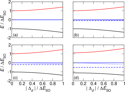
Figure 8: (Color online) Energy fine structure of the S multiplet vs $\left|\Delta_{d}\right|$ for selected values of $\Delta E_{\text{BW}}$. Energies are renormalized to $\Delta E_{\text{SO}}>0$. The selected values of $\Delta E_{\text{BW}}/\left|\Delta E_{\text{SO}}\right|$ are: (a) $0$, (b) $0.1$, (c) $0.2$, (d) $0.5$. The black curve is $E_{-}$, blue dashed is $E_{\text{BW}}$, blue dotted is $E_{<}$, blue solid is $E_{0}\equiv 0$, red is $E_{+}$. For $\Delta E_{\text{BW}}=0$ [case (a)], $E_{\text{BW}}=E_{<}=0=E_{0}$.

Equation (83) shows that the combined action of SO coupling, BW interaction, and disorder produces a non-trivial fine structure made of five resolved energy levels. To study the dependence of the eigenvalues (83) on the different contributions to isospin mixing, we consider ultraclean devices where disorder is a weak perturbation,Kuemmeth08 hence $\left|\Delta_{d}\right|$ is typically much smaller than $\left|\Delta E_{\text{SO}}\right|$. Besides, we have $\left|\Delta E_{\text{BW}}\right|\ll\left|\Delta E_{\text{SO}}\right|$, hence $\left|\Delta E_{\text{SO}}\right|$ is the dominant energy scale that we use to renormalize all energies in Figs. 8 and 9.

Figures 8 and 9 show the energy levels of the S multiplet as a function of $\left|\Delta_{d}\right|/\left|\Delta E_{\text{SO}}\right|$ for selected values of $\Delta E_{\text{BW}}/\left|\Delta E_{\text{SO}}\right|$. Since the distribution of atomic defects is random, here we assume the three quantities $\Delta E_{\text{SO}}$, $\Delta E_{\text{BW}}$, and $\Delta_{d}$ to be uncorrelated, although they all depend on the orbital wave function ($\Delta_{d}$ through the density, $\Delta E_{\text{BW}}$ through the pair correlation function, and $\Delta E_{\text{SO}}$ through the kinetic energy).

Specifically, Fig. 8 focuses on the evolution of the level sequence vs $\Delta_{d}$ with the increase of BW scattering, starting from $\Delta E_{\text{BW}}=0$ [Fig. 8(a)]. We see that BW interaction splits the central line at $E=0$ into two curves, whereas disorder further splits discernibly the zero-energy eigenvalue when $\left|\Delta_{d}\right|/\left|\Delta E_{\text{SO}}\right|>0.4$ [dotted line in Figs. 8(c) and (d)].

In the absence of disorder, the energies of the two outer levels are symmetric with respect to $E=0$. Disorder breaks this symmetry, as shown in Fig. 9. The centroid $(E_{+}+E_{-})$, in fact, deviates from zero as $\Delta_{d}$ increases, although for moderate disorder, say $\left|\Delta_{d}\right|\lesssim 0.2\left|\Delta E_{\text{SO}}\right|$, the discrepancy is small, $(E_{+}+E_{-})\lesssim 10^{-2}\left|\Delta E_{\text{SO}}\right|$.

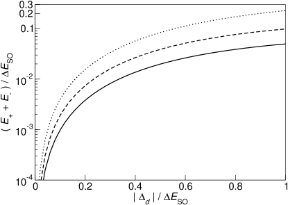
Figure 9: $(E_{+}+E_{-})$ vs $\left|\Delta_{d}\right|$ for selected values of $\Delta E_{\text{BW}}$. Energies are normalized to $\Delta E_{\text{SO}}>0$. The values of $\Delta E_{\text{BW}}/\left|\Delta E_{\text{SO}}\right|$ are: $0.1$ (solid curve), $0.2$ (dashed curve), $0.5$ (dotted curve). For either $\Delta E_{\text{BW}}=0$ or $\Delta_{d}=0$ one has $(E_{+}+E_{-})=0$.

Putting $\Delta_{d}\equiv\left|\Delta_{d}\right|\text{e}^{\text{i}\phi}$, we obtain that the eigenstates associated with eigenvalues $E=E_{+}$, $E_{<}$, and $E_{-}$ are given by

$$\xi_{E} =\Bigg{\{}\frac{E}{E+\Delta E_{\text{BW}}}\left[(\lambda+E)a\,\xi_{0,0}^{(+)}+(\lambda-E)b\,\xi_{0,0}^{(-)}\right]$$

$$\quad\quad-\left|\Delta_{d}\right|\left(\text{e}^{\text{i}\phi}\xi_{0,+2}^{0}+\text{e}^{-\text{i}\phi}\xi_{0,-2}^{0}\right)\Bigg{\}}$$

$$\Bigg{/}\sqrt{2E^{2}\left[1+\frac{\Delta E^{2}_{\text{SO}}}{\left(E+\Delta E_{\text{BW}}\right)^{2}}\right]+2\left|\Delta_{d}\right|^{2}},$$ (86)

the eigenstate of $E_{0}$ is

$$\xi_{0}=\frac{1}{\sqrt{2}}\left(\text{e}^{\text{i}\phi}\xi_{0,+2}^{0}-\text{e}^{-\text{i}\phi}\xi_{0,-2}^{0}\right),$$ (87)

and the two eigenstates corresponding to $E_{\text{BW}}$ are

$$\xi^{\pm}_{E_{\text{BW}}}=\xi^{0}_{\pm 2,0},$$ (88)

as in the absence of disorder.

VIII.3.2 A multiplet

We now consider the ten states of a generic A orbital multiplet, reckoning energies from $E_{\text{A}}+2\epsilon_{d}(\text{A})$. The disorder operator mixes states having like spin projections $\sigma$. Since the probability for the two electrons to be close in space is tiny, we neglect BW scattering.mynote Here we use the notation $\zeta^{\eta}_{\sigma,\tau}$ for the symmetric spin-valley wave functions. The sector with $\sigma=\pm 2$ consists of states $\zeta^{\mp 2}_{\pm 2,-2},\zeta^{0}_{\pm 2,0},\zeta^{\pm 2}_{\pm 2,+2}$. In this subspace, the Hamiltonian matrix is

$$\mathbb{H}(\text{A})^{\sigma=\pm 2}=\left(\begin{matrix}\mp\nu\Delta E_{\text{SO}}&\Delta_{d}^{*}/\sqrt{2}&0\\ \Delta_{d}/\sqrt{2}&0&\Delta_{d}^{*}/\sqrt{2}\\ 0&\Delta_{d}/\sqrt{2}&\pm\nu\Delta E_{\text{SO}}\\ \end{matrix}\right).$$ (89)

The eigenvalues are

$$E_{+}=\sqrt{\Delta E_{\text{SO}}^{2}+\left|\Delta_{d}\right|^{2}}\equiv\lambda_{d},$$

$$E_{0}=0,$$

$$E_{-}=-\sqrt{\Delta E_{\text{SO}}^{2}+\left|\Delta_{d}\right|^{2}}\equiv-\lambda_{d},$$ (90)

and the corresponding eigenstates are

$$\zeta^{(+)}_{\sigma=\pm 2} =\frac{1}{2E_{+}\sqrt{\gamma_{\pm}(\text{A})}}\Big{[}\text{e}^{-\text{i}\phi}\gamma_{\pm}^{2}(\text{A})\zeta^{\mp 2}_{\pm 2,-2}$$

$$+\!\sqrt{2}\left|\Delta_{d}\right|\left(E_{+}-\nu\Delta E_{\text{SO}}\right)\zeta^{0}_{\pm 2,0}+\left|\Delta_{d}\right|^{2}\text{e}^{\text{i}\phi}\zeta^{\pm 2}_{\pm 2,+2}\Big{]},$$

$$\zeta^{(0)}_{\sigma=\pm 2} =\frac{1}{E_{+}}\Big{[}\frac{1}{\sqrt{2}}\left(\Delta^{*}_{d}\zeta^{\mp 2}_{\pm 2,-2}-\Delta_{d}\zeta^{\pm 2}_{\pm 2,+2}\right)$$

$$\pm\nu\Delta E_{\text{SO}}\zeta^{0}_{\pm 2,0}\Big{]},$$

$$\zeta^{(-)}_{\sigma=\pm 2} =\frac{1}{2E_{+}\sqrt{\gamma_{\mp}(\text{A})}}\Big{[}\text{e}^{-\text{i}\phi}\gamma_{\mp}^{2}(\text{A})\zeta^{\mp 2}_{\pm 2,-2}$$

$$-\!\sqrt{2}\left|\Delta_{d}\right|\left(E_{+}+\nu\Delta E_{\text{SO}}\right)\zeta^{0}_{\pm 2,0}+\left|\Delta_{d}\right|^{2}\text{e}^{\text{i}\phi}\zeta^{\pm 2}_{\pm 2,+2}\Big{]},$$ (91)

where we have defined

$$\gamma_{\pm}(\text{A})\equiv\left|\Delta_{d}\right|^{2}+2\Delta E_{\text{SO}}\left(\Delta E_{\text{SO}}\mp\nu E_{+}\right).$$ (92)

The subspace with $\sigma=0$ consists of states $\zeta^{-2}_{0,0},\zeta^{+2}_{0,0},\zeta^{0}_{0,-2},\zeta^{0}_{0,+2}$. In this sector the Hamiltonian matrix is

$$\mathbb{H}(\text{A})^{\sigma=0}=\left(\begin{matrix}-\nu\Delta E_{\text{SO}}&0&\Delta_{d}/2&\Delta_{d}^{*}/2\\ 0&\nu\Delta E_{\text{SO}}&\Delta_{d}/2&\Delta_{d}^{*}/2\\ \Delta_{d}^{*}/2&\Delta_{d}^{*}/2&0&0\\ \Delta_{d}/2&\Delta_{d}/2&0&0\\ \end{matrix}\right).$$ (93)

The eigenvalues are the same as for $\sigma=\pm 2$. The eigenstates are:

$$\zeta_{\sigma=0}^{(+)} =\frac{1}{2\lambda_{d}}\left[\frac{\gamma_{+}(\text{A})\zeta_{0,0}^{-2}+\left|\Delta_{d}\right|^{2}\zeta_{0,0}^{+2}}{\lambda_{d}-\nu\Delta E_{\text{SO}}}\right.$$

$$\left.+\frac{\lambda_{d}-\nu\Delta E_{\text{SO}}}{\sqrt{\gamma_{+}(\text{A})}}\left(\Delta_{d}^{*}\zeta_{0,-2}^{0}+\Delta_{d}\zeta_{0,+2}^{0}\right)\right],$$

$$\zeta_{\sigma=0}^{(0,u)} =\frac{1}{\sqrt{2}}\left(\text{e}^{-\text{i}\phi}\zeta_{0,-2}^{0}-\text{e}^{\text{i}\phi}\zeta_{0,+2}^{0}\right),$$

$$\zeta_{\sigma=0}^{(0,g)} =\frac{1}{\sqrt{2}\lambda_{d}}\left[\left|\Delta_{d}\right|\left(\zeta_{0,0}^{-2}-\zeta_{0,0}^{+2}\right)\right.$$

$$\left.+\nu\Delta E_{\text{SO}}\left(\text{e}^{-\text{i}\phi}\zeta_{0,-2}^{0}+\text{e}^{\text{i}\phi}\zeta_{0,+2}^{0}\right)\right],$$

$$\zeta_{\sigma=0}^{(-)} =\frac{1}{2\lambda_{d}}\left[\frac{\gamma_{-}(\text{A})\zeta_{0,0}^{-2}+\left|\Delta_{d}\right|^{2}\zeta_{0,0}^{+2}}{\lambda_{d}+\nu\Delta E_{\text{SO}}}\right.$$

$$\left.-\frac{\lambda_{d}+\nu\Delta E_{\text{SO}}}{\sqrt{\gamma_{-}(\text{A})}}\left(\Delta_{d}^{*}\zeta_{0,-2}^{0}+\Delta_{d}\zeta_{0,+2}^{0}\right)\right],$$ (94)

where the apex $(0,g)$ [$(0,u)$] labels the eigenspace with $E_{0}=0$ corresponding to the (anti)symmetric combination of states of opposite isospins (in the absence of disorder).

IX Conclusion

In conclusion, we have provided a theory of inter-valley scattering induced by Coulomb interaction in semiconducting carbon-nanotube quantum dots, which takes explicitly into account tube chirality. Focusing on two electrons, we have shown that BW scattering depends on the pair correlation function of the interacting state. We have predicted previously overlooked energy splittings of the order of some tens of $\mu$eV in the fine structure of the lowest symmetric orbital multiplet in typical regimes, whereas the effect of BW interaction is negligible for antisymmetric orbital wave functions.

As a by-product, we have presented analytical expressions for the atomic coordinates on an arbitrary CNT surface that depend on two indexes unrelated to the graphene geometry. This could be useful for evaluating microscopic and mechanical properties of CNTs.

We have included in our model the effect of short-range disorder due to a random distribution of atomic defects, being an additional source of inter-valley scattering. The interplay between SO coupling, BW scattering and disorder leads to a rich energy spectrum for S multiplets. In particular, two-electron states are no more eigenstates of the isospin, which has implications for the studies of spin-valley blockade. Our findings are useful for the interpretation of Coulomb blockade experiments in ultraclean carbon nanotubes as well as for designing two-electron qubits.

Appendix A Atomic coordinates

In this Appendix we detail the derivation of Eqs. (8) and (9), starting from Eq. (7). Within sublattice A (B), we first determine the allowed axial coordinates $y_{\text{A}}$ ($y_{\text{B}}$), expressed as a function of the integer number $n$, and then determine the angular coordinate $\theta_{\text{A}}$ ($\theta_{\text{B}}$) of all the atoms located on the tube circumference at $y_{\text{A}}$ ($y_{\text{B}}$).

A.1 Axial coordinate

The axial coordinate $y_{\text{A}}(n_{1},n_{2})$ [$y_{\text{B}}(n_{1},n_{2})$] appearing in Eq. (7) may be put in one-to-one correspondence with the integer index $n$, varying in $(-\infty,+\infty)$ if the nanotube length is infinite. In order to show this we write

$$n_{a}\equiv f_{ab}\nu_{a},\quad n_{b}\equiv f_{ab}\nu_{b},$$ (95)

where $f_{ab}$ is the greatest common divisor of $n_{a}$ and $n_{b}$, and the integers $\nu_{a}$ and $\nu_{b}$ are coprime. Simplifying Eq. (7) accordingly, we obtain

$$y_{\text{A}}(n_{1},n_{2})=y_{\text{B}}(n_{1},n_{2})+\Delta y_{\text{AB}},$$

$$y_{\text{B}}(n_{1},n_{2})=\frac{\sqrt{3}a}{2\sqrt{\nu^{2}_{a}+\nu^{2}_{b}-\nu_{a}\nu_{b}}}\Big{(}\nu_{a}n_{2}-\nu_{b}n_{1}\Big{)},$$ (96)

where

$$\Delta y_{\text{AB}}=\frac{\sqrt{3}a}{2\sqrt{\nu_{a}^{2}+\nu_{b}^{2}-\nu_{a}\nu_{b}}}\frac{1}{3}\Big{(}2\nu_{a}-\nu_{b}\Big{)}=\frac{a}{\sqrt{3}}\cos(\alpha).$$ (97)

The allowed values of the axial coordinate depend on those assumed by the integer quantity $(\nu_{a}n_{2}-\nu_{b}n_{1})$, with both $n_{1}$ and $n_{2}$ belonging to $\mathbb{Z}$. To find out these values, we use a result of discrete mathematics known as Bézout’s lemma:Tignol01 If $a$ and $b$ are non-zero integers with greatest common divisor $d$, then there exist two integers $n_{x}$ and $n_{y}$ such that $an_{x}+bn_{y}=d$. Hence, replace $a$, $b$ and $d$, respectively, by $\nu_{a}$, $\nu_{b}$, and $1$. This lemma implies that there exists a couple $(n^{*}_{1},n^{*}_{2})$ such that $\nu_{a}n^{*}_{2}-\nu_{b}n^{*}_{1}=1$. It follows that for any integer $n$, there is a couple of integers $(n_{1}=nn^{*}_{1},n_{2}=nn^{*}_{2})$ such that $\nu_{a}n_{2}-\nu_{b}n_{1}=n$. In other words, the domain for the quantity $(\nu_{a}n_{2}-\nu_{b}n_{1})$ is the whole $\mathbb{Z}$. It follows that the allowed axial coordinates of the carbon atoms may be written as

$$y_{\text{A}}(n)=y_{\text{B}}(n)+\Delta y_{\text{AB}},$$

$$y_{\text{B}}(n)=\frac{\sqrt{3}a}{2\sqrt{\nu^{2}_{a}+\nu^{2}_{b}-\nu_{a}\nu_{b}}}n,$$ (98)

for any $n\in\mathbb{Z}$.

A.2 Angular coordinate

We proceed to identify the atoms lying on the nanotube circumference at the axial coordinate $y_{\text{A}}(n)$ [$y_{\text{B}}(n)]$. Consider two sites of the B sublattice at $\underline{R}_{\text{B}}\equiv\underline{R}_{\text{B}}(n_{1},n_{2})$ and $\underline{R}^{\prime}_{\text{B}}\equiv\underline{R}_{\text{B}}(n^{\prime}_{1},n^{\prime}_{2})$. From Eqs. (96), the two sites have the same axial coordinate if

$$y_{\text{B}}=y^{\prime}_{\text{B}}\Rightarrow\nu_{a}(n_{2}-n^{\prime}_{2})=\nu_{b}(n_{1}-n^{\prime}_{1}),$$ (99)

with an analogous condition for A sublattice. Since $\nu_{a}$ and $\nu_{b}$ are coprime, condition (99) holds if there exists an integer $\bar{n}$ such that

$$\left\{\begin{matrix}n_{2}-n^{\prime}_{2}=\bar{n}\nu_{b}\\ n_{1}-n^{\prime}_{1}=\bar{n}\nu_{a}\end{matrix}\right..$$ (100)

On the other hand, the difference between the two angular coordinates is:

$$\theta_{\text{B}}\!-\theta^{\prime}_{\text{B}} =\!\left\{\!\pi\frac{\left(2\nu_{a}-\nu_{b}\right)\!\left(n_{1}-n^{\prime}_{1}\right)+\left(2\nu_{b}-\nu_{a}\right)\!\left(n_{2}-n^{\prime}_{2}\right)}{f_{ab}\left(\nu^{2}_{a}+\nu^{2}_{b}-\nu_{a}\nu_{b}\right)}\!\right\}$$

$$\mod(2\pi).$$ (101)

Substituting the condition (100) into (101), we obtain that the angular distance between two B sites with the same axial coordinate is

$$\Big{[}\theta_{\text{B}}-\theta^{\prime}_{\text{B}}\Big{]}\Bigg{|}_{y_{\text{L}}=y^{\prime}_{\text{L}}}=\frac{2\pi}{f_{ab}}\bar{n}\mod(2\pi).$$ (102)

This shows that there are $f_{ab}$ distinct sublattice atoms on the nanotube circumference [obtained for $\bar{n}=0,1,\ldots(f_{ab}-1)$], with the angular distance between two first neighbours given by $2\pi/f_{ab}$. To summarize, atoms belonging to a given sublattice are identified by two integers: $n\in\mathbb{Z}$, specifying the axial coordinate $y_{p}(n)$ plus an angular offset [cf. Eq. (8)], and $j\in\{0,1,\ldots,f_{ab}-1\}$, labelling the $f_{ab}$ atoms lying on the $y=y_{p}(n)$ cross section.

Suppose now that the couple $(\bar{n}_{1},\bar{n}_{2})$ specifies an atom lying on the tube circumference at $y=y_{B}(1)$. From Eq. (96), this means that $\nu_{a}\bar{n}_{2}-\nu_{b}\bar{n}_{1}=1$. Then, the couple $(n_{1}=n\bar{n}_{1},n_{2}=n\bar{n}_{2})$, for any arbitrary $n$, specifies an atom lying on the circumference at $y=y_{B}(n)$, since $\nu_{a}n_{2}-\nu_{b}n_{1}=n$. Therefore, the task of determining the allowed angular coordinates reduces to finding a couple $(\bar{n}_{1},\bar{n}_{2})$ satisfying $\nu_{a}\bar{n}_{2}-\nu_{b}\bar{n}_{1}=1$: once this is done, we compute the quantity

$$\theta_{\text{B}}(1)\equiv\pi\frac{\nu_{a}\left(2\bar{n}_{1}-\bar{n}_{2}\right)-\nu_{b}\left(\bar{n}_{1}-2\bar{n}_{2}\right)}{f_{ab}\left(\nu_{a}^{2}+\nu_{b}^{2}-\nu_{a}\nu_{b}\right)}$$ (103)

and we obtain all the angular coordinates of the atoms of the B sublattice as

$$\theta_{\text{B}}(\bar{n}_{1},\bar{n}_{2})=\theta_{\text{B}}(1)\mod(2\pi),$$

$$\theta_{\text{B}}(n_{1},n_{2})=[n\theta_{\text{B}}(1)]\mod(2\pi),$$ (104)

where $(n_{1},n_{2})=(n\bar{n}_{1},n\bar{n}_{2})$. Finally, the couple $(\bar{n}_{1},\bar{n}_{2})$ needed to evaluate $\theta_{\text{B}}(1)$ can be obtained by applying directly the extended Euclidean algorithm. Combining Eqs. (97), (98), (103) and (104), and considering the offset between A and B angular coordinates that can be evaluated directly from (7), we obtain the expressions (8) and (9).

Appendix B Single-particle states

In this Appendix we recall the properties of the eigenstates of the one-electron Hamiltonian of a quantum dot embedded in a semiconducting carbon nanotube.

B.1 Energy dispersion and Bloch states

The energy dispersion $\varepsilon_{\pm}({\bf{k}})$ of graphene conduction ($+$) and valence ($-$) bands in the proximity of the non-equivalent special points $\bf{K}$ and $\bf{K}^{\prime}$ of the first Brillouin zone is characterized by the occurrence of Dirac cones:CastroNeto09

$$\varepsilon_{\pm}({\bf{k}})\cong\left\{\begin{matrix}\pm\gamma\left|{\bf{k}}-{\bf{K}}\right|\quad\text{for }{\bf{k}}\approx{\bf{K}}\\ \pm\gamma\left|{\bf{k}}-{\bf{K}^{\prime}}\right|\quad\text{for }{\bf{k}}\approx{\bf{K}^{\prime}}\end{matrix}\right.,$$ (105)

where $\gamma\cong 533\text{ meV}\cdot\text{nm}$ is the $\pi$-band parameter of graphene, and ${\bf{k}}=k_{x}\overrightarrow{\bf{x}}+k_{y}\overrightarrow{\bf{y}}$. The dispersion (105), due to the honeycomb lattice of graphene,Wallace47 may be derived most simply by applying the tight-binding method, building Bloch states as superpositions of atomic orbitals centered on the sublattice sites. If the orbital hybridization induced by the CNT curvature is neglected, one may use graphene band structure to derive the energy bands of CNTs. This is reduced to applying a simple folding procedure to take into account the CNT cylinder topology.DresselhausBook

We write the direct-space vectors lying on the CNT surface as ${\bf{R}}_{p}\equiv\left(R,\underline{R}_{p}\right)$, $p\in\{\text{A, B}\}$, with $\underline{R}_{p}\equiv\left(\theta_{p},y_{p}\right)$ and $R$ fixed. Using the azimuthal and axial coordinates, chiral and translation vectors are $\underline{L}=(2\pi,0)$ and $\underline{T}=(0,T)$ [note the bar symbol labelling vectors in the $\left(\theta,y\right)$ frame]. We introduce generalized wave vectors of the form $\underline{k}\equiv\left(\kappa,k\right)$, where $\kappa$ is the dimensionless wave vector along the nanotube circumference ($\kappa=k_{x}R$) and $k$ is the wave vector along the nanotube axis (with the dimension of the inverse of a length). The scalar product between $\underline{k}$ and generalized position vectors, of the form $\underline{r}\equiv\left(\theta,y\right)$, is defined as $\underline{k}\cdot\underline{r}=\kappa\theta+ky$. Sublattice Bloch states DresselhausBook in CNTs are written as

$$\psi_{p}(\underline{k},{\bf{r}})=\text{e}^{\text{i}\theta_{p}(\underline{k})}\frac{1}{\sqrt{N_{c}}}\sum_{{\bf{R}}_{p}}\text{e}^{\text{i}\underline{k}\cdot\underline{R}_{p}}\phi_{2p_{z}}\!\!\left({\bf{r}}-{\bf{R}}_{p}\right),$$ (106)

where $p\in\{\text{A},\text{B}\}$, $\phi_{2p_{z}}\!\!\left({\bf{r}}-{\bf{R}}_{p}\right)$ is a single-particle $\pi$-band orbital centered at ${\bf{R}}_{p}$, $\theta_{p}(\underline{k})$ is a phase factor depending on $\underline{k}$, and $N_{c}$ is the number of sublattice sites of the CNT (i.e., the number of curved hexagons made of two carbon atoms each). We assume $2p_{z}$ atomic orbitals to be normalized as

$$\int_{\text{CNT}}\left|\phi_{2p_{z}}\!\!\left({\bf{r}}-{\bf{R}}_{p}\right)\right|^{2}\text{d}{\bf{r}}=\mathcal{V}_{\text{CNT}},$$ (107)

where the integration is over the whole CNT and $\mathcal{V}_{\text{CNT}}=(2\pi R)L_{y}L_{z}$, where $L_{y}$ is the CNT length and $L_{z}$ is the characteristic length associated with $2p_{z}$ orbitals. Secchi10

The proviso to include the effect of CNT curvature into the band structure is that wave functions trasform into themselves under a $2\pi$-rotation around the axis, $\underline{r}\rightarrow\underline{r}+\underline{L}$, which restricts the allowed values of the circumferential wave vector $\kappa$ to integer values. This condition singles out a set of one-dimensional energy subbands, one subband for each value of $\kappa=n$,DresselhausBook ; AndoReview which are the sections of the Dirac cones at $k_{x}(n)=n/R$. The intersections closest to graphene high-symmetry points $\bf{K}$ and $\bf{K}^{\prime}$ exhibit conduction-band absolute minima and valence-band maxima. These extremal points occur at the following wave vectors:

$$\underline{M}=\left(\frac{n_{a}+n_{b}-\nu}{3},\frac{n_{a}-n_{b}}{\sqrt{3}R}\right),$$

$$\underline{M}^{\prime}=\left(\frac{2n_{a}-n_{b}+\nu}{3},\frac{-n_{b}}{\sqrt{3}R}\right),$$ (108)

where $\nu\in\{-1,0,+1\}$ is such that $n_{a}+n_{b}=3n^{*}+\nu$, and $n^{*}$ is the integer closest to $(n_{a}+n_{b})/3$. The $\kappa$ components of $\underline{M}$ and $\underline{M}^{\prime}$ are integer numbers (respectively, $M_{\kappa}=n^{*}$ and $M^{\prime}_{\kappa}=n_{a}-n^{*}$), labelling the two one-dimensional bands in which the conduction-band minima lie.

The number $\nu$ determines the electronic properties of the nanotube: if $\nu=0$, the nanotube is a metal, while if $\nu=\pm 1$ the nanotube is a semiconductor. We label the two non-equivalent minima by means of the isospin index $\tau=+1$ $(-1)$ for point $\underline{M}$ $(\underline{M}^{\prime})$. The Bloch states corresponding to the conduction-band minima are given by Secchi10

$$\psi_{\tau}({\bf{r}})=\sum_{p=\text{A,B}}\!\!f^{p}_{\tau}\text{e}^{\text{i}\theta^{p}_{\tau}}\frac{1}{\sqrt{N_{c}}}\sum_{{\bf{R}}_{p}}\text{e}^{\text{i}\underline{M}_{\tau}\cdot\underline{R}_{p}}\phi_{2p_{z}}\!\left({\bf{r}}-{\bf{R}}_{p}\right),$$ (109)

where coefficients are given byAndo98

$$f^{\text{A}}_{+1}=1,\quad f^{\text{B}}_{+1}=\nu,\quad f^{\text{A}}_{-1}=1,\quad f^{\text{B}}_{-1}=-\nu,$$

$$\theta^{\text{A}}_{+1}=0,\quad\theta^{\text{B}}_{+1}=\alpha+5\pi/3,\quad\theta^{\text{A}}_{-1}=\alpha,\quad\theta^{\text{B}}_{-1}=0.$$ (110)

Explicitly, the CNT dispersion, close to the charge neutrality points, is:

$$\varepsilon_{\pm}(\tau,n,k_{y})=\pm\gamma\sqrt{\left[k_{x}(n)_{\tau}\right]^{2}+k_{y}^{2}},$$ (111)

where the $k_{x}$ and $k_{y}$ wave vectors are now reckoned from $\bf{K}$ and $\bf{K}^{\prime}$ in valleys $\tau=+1$ and $\tau=-1$, respectively. The quantized circumferential wave vector is

$$k_{x}(n)_{\tau}\equiv\frac{1}{R}\left(n-\frac{\nu\tau}{3}\right),$$ (112)

where $n\in\{0,\pm 1,\pm 2,\ldots\}$. Note the difference between the two vectors $k_{x}(n)_{\tau}$ and $k_{x}(n)=n/R$.

B.2 Spin-orbit coupling

Spin-orbit coupling is the first-order relativistic correction to the Hamiltonian and has a topological origin in CNTs due to their curvature, as established both theoreticallyAndo00 ; HuertasHernando06 ; Zhou09 ; Chico09 ; Jeong09 ; Izumida09 and experimentally.Kuemmeth08 ; Churchill09 ; Jhang10 ; Jespersen11 ; Steele13 Even in the absence of external magnetic fields the combined spin and isospin fourfold degeneracy of one-electron states is lifted, originating two Kramers doublets, each one composed of two levels sharing the same value of the product $\eta\equiv\sigma\tau=\pm 1$.

Including SO, the CNT dispersion may be written asAndo00 ; HuertasHernando06 ; Zhou09 ; Chico09 ; Jeong09 ; Izumida09 ; Jespersen11

$$\varepsilon_{\pm}(\sigma,\tau,n,k_{y})=\Delta_{\text{SO}}^{(0)}\cos(3\alpha)\frac{\gamma}{R}\sigma\tau\pm\gamma\sqrt{\left[k_{x}(n)_{\sigma\tau}\right]^{2}+k_{y}^{2}}.$$ (113)

Here $k_{x}$ depends on SO coupling,

$$k_{x}(n)_{\sigma\tau}\equiv\frac{1}{R}\left(n-\frac{\nu\tau}{3}\right)-\sigma\frac{\Delta^{(1)}_{\text{SO}}}{R},$$ (114)

where $\Delta^{(0)}_{\text{SO}}$ and $\Delta^{(1)}_{\text{SO}}$ are two spin-orbit dimensionless parameters of the same order of magnitude, $\left|\Delta^{(0)}_{\text{SO}}\right|\approx\left|\Delta^{(1)}_{\text{SO}}\right|\approx 10^{-3}$. While the existence of the $\Delta^{(1)}_{\text{SO}}$ term was predicted long ago,Ando00 the occurrence of the $\Delta_{\text{SO}}^{(0)}$ term was proposed only recently.Zhou09 ; Chico09 ; Jeong09 ; Izumida09 The $\Delta^{(0)}_{\text{SO}}$ term has the same sign for electrons and holes, therefore it breaks the electron-hole symmetry, i.e., $\varepsilon_{-}(\sigma,\tau,n,k_{y})\neq-\varepsilon_{+}(\sigma,\tau,n,k_{y})$, consistently with its experimental observation.Kuemmeth08 In the following, we will show how the theoretical formalism that we have employed in our previous worksSecchi09 ; Secchi10 ; Secchi12 ; Pecker13 may be extended to account for the new term $\Delta_{\text{SO}}^{(0)}$, as well as for the coupling with the axial orbital degree of freedom $y$, as recently observed.Jespersen11

B.3 Effective mass approximation

We now introduce a confinement potential that forms a 1D QD, varying slowly with respect to the scale of $a$. We focus on semiconducting CNTs, treating the low-energy states close to the charge neutrality point using the envelope functions in the effective mass approximation.Luttinger55 This is obtained by expanding (113) for $k_{y}^{2}\ll\left[k_{x}(n)_{\sigma\tau}\right]^{2}$, retaining only terms up to order $\left[k_{y}/k_{x}(n)_{\sigma\tau}\right]^{2}$. Therefore,

$$\sqrt{\left[k_{x}(n)_{\sigma\tau}\right]^{2}+k_{y}^{2}}\approx\left|k_{x}(n)_{\sigma\tau}\right|+\frac{k_{y}^{2}}{2\left|k_{x}(n)_{\sigma\tau}\right|}.$$ (115)

We consider only $n=0$, corresponding to the lowest subband for both electrons and holes. We have

$$\left|k_{x}(0)_{\sigma\tau}\right|=\frac{1}{R}\left|\frac{\nu\tau}{3}+\Delta_{\text{SO}}^{(1)}\sigma\right|=\frac{1}{3R}+\frac{\Delta_{\text{SO}}^{(1)}}{R}\nu\sigma\tau,$$ (116)

since $\left|\nu\tau\right|=1$ for semiconducting CNTs ($\nu=\pm 1$), and $\left|\Delta_{\text{SO}}^{(1)}\right|\ll 1/3$. Therefore, the conduction and valence bands (113) may be approximated as:

$$\varepsilon_{\pm}\cong\pm\frac{\gamma}{3R}+\frac{\Delta_{\text{SO}\pm}\gamma}{R}\nu\sigma\tau\pm\frac{1}{2}\frac{3R\gamma}{1+3\Delta_{\text{SO}}^{(1)}\nu\sigma\tau}k_{y}^{2},$$ (117)

where $\Delta_{\text{SO}\pm}\equiv\nu\Delta_{\text{SO}}^{(0)}\cos(3\alpha)\pm\Delta_{\text{SO}}^{(1)}$. Now we make the operatorial substitution $k_{y}^{2}\rightarrow-\partial^{2}/\partial y^{2}$ and define the spin- and isospin-dependent effective mass $m^{*}_{\sigma\tau}$ as

$$m^{*}_{\sigma\tau}\equiv\frac{\hbar^{2}}{3R\gamma}\left(1+3\Delta_{\text{SO}}^{(1)}\nu\sigma\tau\right).$$ (118)

Focusing on the conduction band, we write the effective single-particle Hamiltonian $H_{\text{SP}}$, including the QD confinement potential $V_{\text{QD}}(y)$, as

$$H_{\text{SP}}=\frac{\gamma}{3R}+\frac{\Delta_{\text{SO}+}\gamma}{R}\nu\sigma\tau-\frac{\hbar^{2}}{2m^{*}_{\sigma\tau}}\frac{\partial^{2}}{\partial y^{2}}+V_{\text{QD}}(y).$$ (119)

We note from Eq. (118) that the spin- and isospin- dependent part of $m^{*}_{\sigma\tau}$ is of the order of $\approx 10^{-3}m^{*}$, where $m^{*}$ is the orbital effective mass,

$$m^{*}\equiv\frac{\hbar^{2}}{3R\gamma}.$$ (120)

Therefore, we can expand $1/m^{*}_{\sigma\tau}$ in Eq. (119) to the first order in $\Delta_{\text{SO}}^{(1)}$, obtaining

$$H_{\text{SP}}\cong \frac{\gamma}{3R}+\nu\sigma\tau\left(\frac{\Delta_{\text{SO}+}\gamma}{R}+3\Delta_{\text{SO}}^{(1)}\frac{\hbar^{2}}{2m^{*}}\frac{\partial^{2}}{\partial y^{2}}\right)$$

$$-\frac{\hbar^{2}}{2m^{*}}\frac{\partial^{2}}{\partial y^{2}}+V_{\text{QD}}(y).$$ (121)

In the case of a gate-defined QD embedded in a CNT the confinement potential is parabolic:

$$V_{\text{QD}}(y)=\frac{1}{2}m^{*}\omega_{0}^{2}y^{2},$$ (122)

with $\omega_{0}$ being the characteristic harmonic oscillator frequency. The QD size in real space is given by the characteristic length $\ell_{\text{QD}}=\sqrt{\hbar/(m^{*}\omega_{0})}$.

A QD single-particle state is the product of the microscopic Bloch function (109) times the slowly-varying envelope function $F_{n\tau\sigma}(y)$ times the spinor $\chi_{\sigma}$,

$$\psi_{n\tau\sigma}({\bf{r}},s)=\mathcal{N}F_{n\sigma\tau}(y)\psi_{\tau}({\bf{r}})\chi_{\sigma}(s),$$ (123)

where $\mathcal{N}$ is a normalization constant that will be specified later. The envelope function $F_{n\sigma\tau}(y)$ satisfies the eigenvalue equation

$$H_{\text{SP}}F_{n\tau\sigma}=\epsilon_{n\tau\sigma}F_{n\tau\sigma},$$ (124)

with $n$ labelling the orbital states. For simplicity, we use again first-order perturbation theory, assuming that the orbital functions do not depend on $\sigma$ and $\tau$. Therefore, we assume that $F_{n}$ solves the eigenvalue problem

$$\left[-\frac{\hbar^{2}}{2m^{*}}\frac{\partial^{2}}{\partial y^{2}}+V_{\text{QD}}(y)\right]F_{n}(y)=\epsilon_{n}F_{n}(y),$$ (125)

where $\epsilon_{n}$ is a QD discrete level and the envelope function normalization is

$$\int_{-\infty}^{+\infty}F^{*}_{n}(y)F_{n^{\prime}}(y)\text{d}y=\ell_{\text{QD}}\delta_{n,n^{\prime}}.$$ (126)

The orbital envelope function can be multiplied by the four microscopic states $\psi_{\tau}({\bf{r}})\chi_{\sigma}(s)$, with $\tau\in\{+1,-1\}$ and $\sigma\in\{+1,-1\}$. Each one of these states has energy $\varepsilon_{n\tau\sigma}$, with

$$\varepsilon_{n\tau\sigma} =\frac{\gamma}{3R}+\varepsilon_{n}+\left(\frac{\Delta_{\text{SO}+}\gamma}{R}-3\Delta_{\text{SO}}^{(1)}\left<E_{n}^{\text{kin}}\right>\right)\nu\sigma\tau$$

$$\equiv\frac{\gamma}{3R}+\varepsilon_{n}+\frac{\Delta_{\text{SO}}\gamma}{R}\nu\sigma\tau,$$ (127)

and

$$\left<E_{n}^{\text{kin}}\right>=-\frac{\hbar^{2}}{2m^{*}}\ell_{\text{QD}}^{-1}\int_{-\infty}^{+\infty}F^{*}_{n}(y)\frac{\partial^{2}}{\partial y^{2}}F_{n}(y)\text{d}y$$ (128)

is a kinetic-energy correction to the effective spin-orbit parameter,

$$\Delta_{\text{SO}}\equiv\Delta_{\text{SO}+}-3\Delta_{\text{SO}}^{(1)}\frac{R\left<E_{n}^{\text{kin}}\right>}{\gamma}.$$ (129)

According to Eq. (127), the single-particle orbital energy $\varepsilon_{n\tau\sigma}$ is split into two levels, corresponding respectively to $\sigma\tau=+1$ and $\sigma\tau=-1$. The gap between such states is $2\Delta_{\text{SO}}\gamma/R$, where, as shown by Eq. (129), the SO parameter $\Delta_{\text{SO}}$ varies with the orbital multiplet under consideration through the kinetic term (128). This effect has also been observed experimentally: Jespersen11 in particular, it has been shown that the SO gap changes as the confinement potential is modified by an electrostatic gate. In the following we will just take $\Delta_{\text{SO}}$ as a parameter, keeping in mind that it can change in magnitude and sign with the orbital multiplet under consideration.

Finally, the normalization constant $\mathcal{N}$ in Eq. (123) is evaluated with a procedure Secchi10 that exploits the localization of the atomic orbitals $\phi_{2p_{z}}$ appearing in the Bloch states (109) around the positions of the respective carbon nuclei; the result is

$$\mathcal{N}=\frac{1}{2\sqrt{\pi RL_{z}\ell_{\text{QD}}}},$$ (130)

providing the following normalization of the orbital wave functions:

$$\mathcal{N}^{2}\int_{\text{CNT}}\left[F^{*}_{n}(y)\psi^{*}_{\tau}({\bf{r}})\right]\left[F_{n^{\prime}}(y)\psi_{\tau^{\prime}}({\bf{r}})\right]\text{d}{\bf{r}}=\delta_{n,n^{\prime}}\delta_{\tau,\tau^{\prime}}.$$ (131)

Appendix C The BW scattering term of the Hamiltonian

In this Appendix we detail the passages that lead from the expression (15) to the form (18) of BW scattering matrix elements.

Using Eqs. (17) and (20), we write (15) as

$$V^{(\text{BW})}_{a,b;c,d}(\tau)=\frac{L_{y}^{2}}{4N_{c}^{2}}\ell_{\text{QD}}^{-2}\sum_{p,p^{\prime}}\text{e}^{\text{i}\tau\phi_{pp^{\prime}}}\sum_{n\in\mathbb{Z}}\sum_{j=0}^{f_{ab}-1}\sum_{n^{\prime}\in\mathbb{Z}}\sum_{j^{\prime}=0}^{f_{ab}-1}$$

$$\text{e}^{\text{i}\tau\Delta M_{\kappa}\cdot\left[\theta_{p}(n,j)-\theta_{p^{\prime}}(n^{\prime},j^{\prime})\right]}\text{e}^{\text{i}\tau\Delta M_{k}\cdot\left[y_{p}(n)-y_{p^{\prime}}(n^{\prime})\right]}$$

$$\times U\!\left\{\left[y_{p}(n)-y_{p^{\prime}}(n^{\prime})\right]^{2},\sin^{2}\!\left[\frac{\theta_{p}(n,j)-\theta_{p^{\prime}}(n^{\prime},j^{\prime})}{2}\right]\right\}$$

$$\times F_{a}^{*}[y_{p}(n)]F_{b}^{*}[y_{p^{\prime}}(n^{\prime})]F_{c}[y_{p^{\prime}}(n^{\prime})]F_{d}[y_{p}(n)].$$ (132)

To simplify this expression, we note that it contains both quantities that vary slowly (the envelope functions) and quantities that vary rapidly (the exponentials and the interaction potential) with respect to the indexes $n$ and $n^{\prime}$ labelling the axial coordinates. Nevertheless, the dependence of the rapidly-varying quantities on the axial coordinates occurs through the difference

$$y_{p}(n)-y_{p^{\prime}}(n^{\prime})=\Delta y_{pp^{\prime}}+y_{\text{B}}(n-n^{\prime}),$$ (133)

with $\Delta y_{\text{BA}}=-\Delta y_{\text{AB}}$, and $\Delta y_{\text{AA}}=\Delta y_{\text{BB}}=0$, hence the expression on the left hand side of (133) depends only on $(n-n^{\prime})$.

Now consider the dependence of the expression (132) on the angular coordinates, namely on the quantity $\theta_{p}(n,j)-\theta_{p^{\prime}}(n^{\prime},j^{\prime})$. This must be investigated with some care. Below we show that, if $p=p^{\prime}$, the angular difference is an angle pointing to the B sublattice, otherwise it points to the A sublattice. This is seen most easily by considering the representation of angles in terms of indexes $(n_{1},n_{2})$, Eq. (7). Specifically, given $(n,j)$ and $(n^{\prime},j^{\prime})$, consider two couples $(\bar{n}_{1},\bar{n}_{2})$ and $(\bar{n}^{\prime}_{1},\bar{n}^{\prime}_{2})$ such that

$$y_{p}(\bar{n}_{1},\bar{n}_{2})=y_{p}(n),\quad\theta_{p}(\bar{n}_{1},\bar{n}_{2})=\theta_{p}(n,j),$$

$$y_{p^{\prime}}(\bar{n}^{\prime}_{1},\bar{n}^{\prime}_{2})=y_{p^{\prime}}(n^{\prime}),\quad\theta_{p^{\prime}}(\bar{n}^{\prime}_{1},\bar{n}^{\prime}_{2})=\theta_{p^{\prime}}(n^{\prime},j^{\prime}).$$ (134)

We need to evaluate

$$\theta_{p}(n,j)-\theta_{p^{\prime}}(n^{\prime},j^{\prime})=\theta_{p}(\bar{n}_{1},\bar{n}_{2})-\theta_{p^{\prime}}(\bar{n}^{\prime}_{1},\bar{n}^{\prime}_{2}).$$ (135)

We distinguish two possibilities: $p=p^{\prime}$ and $p\neq p^{\prime}$.

We first show that, if $p=p^{\prime}$, (135) is equal to

$$\theta_{p}(\bar{n}_{1},\bar{n}_{2})-\theta_{p}(\bar{n}^{\prime}_{1},\bar{n}^{\prime}_{2})=\theta_{\text{B}}(\bar{n}_{1}-\bar{n}^{\prime}_{1},\bar{n}_{2}-\bar{n}^{\prime}_{2})+2\pi m$$ (136)

for some integer $m$. Certainly, one of the axial coordinates consistent with the angle $\theta_{\text{B}}(\bar{n}_{1}-\bar{n}^{\prime}_{1},\bar{n}_{2}-\bar{n}^{\prime}_{2})$ is

$$y_{\text{B}}(\bar{n}_{1}-\bar{n}^{\prime}_{1},\bar{n}_{2}-\bar{n}^{\prime}_{2}) =y_{p}(\bar{n}_{1},\bar{n}_{2})-y_{p}(\bar{n}^{\prime}_{1},\bar{n}^{\prime}_{2})$$

$$=y_{p}(n)-y_{p}(n^{\prime})=y_{\text{B}}(n-n^{\prime}).$$ (137)

This means that there exist integers $j^{*}$ and $q$, depending on $j$ and $j^{\prime}$, such that

$$\theta_{p}(n,j)-\theta_{p}(n^{\prime},j^{\prime})=\theta_{\text{B}}[n-n^{\prime},j^{*}(j,j^{\prime})]+2\pi q(j,j^{\prime}),$$ (138)

where $j^{*}$ is not necessarily equal to $j-j^{\prime}$, but it can be constrained to lie in the interval $\{0,\ldots,f_{ab}-1\}$ by means of an appropriate choice of $q$. Since we must evaluate the following double sum in (132),

$$v_{pp}\equiv \sum_{j=0}^{f_{ab}-1}\sum_{j^{\prime}=0}^{f_{ab}-1}\text{e}^{\text{i}\tau\Delta M_{\kappa}\cdot\left[\theta_{p}(n,j)-\theta_{p}(n^{\prime},j^{\prime})\right]}$$

$$\times U\left\{\left[y_{\text{B}}(n-n^{\prime})\right]^{2},\sin^{2}\left[\frac{\theta_{p}(n,j)-\theta_{p}(n^{\prime},j^{\prime})}{2}\right]\right\},$$ (139)

it is easy to see that, for every fixed $j$, as $j^{\prime}$ varies in $\{0,\ldots,f_{ab}-1\}$, the quantity $j^{*}(j,j^{\prime})$ in eq. (138) may be let to vary in the same interval $\{0,\ldots,f_{ab}-1\}$ by appropriately choosing the integers $q(j,j^{\prime})$. The key observation is that the actual values of $q(j,j^{\prime})$ do not matter in the evaluation of eq. (139), since $\Delta M_{\kappa}$ is an integer number and the interaction potential is periodic in the angular coordinates. So, the quantity (139) is equal to:

$$v_{pp}= f_{ab}\sum_{j=0}^{f_{ab}-1}\text{e}^{\text{i}\tau\Delta M_{\kappa}\cdot\theta_{\text{B}}(n-n^{\prime},j)}$$

$$\times U\left\{\left[y_{\text{B}}(n-n^{\prime})\right]^{2},\sin^{2}\left[\frac{\theta_{\text{B}}(n-n^{\prime},j)}{2}\right]\right\}.$$ (140)

We now consider Eq. (135) for $p\neq p^{\prime}$. If $p=\text{A}$ and $p^{\prime}=\text{B}$, we obtain

$$\theta_{\text{A}}(\bar{n}_{1},\bar{n}_{2})-\theta_{\text{B}}(\bar{n}^{\prime}_{1},\bar{n}^{\prime}_{2})=\theta_{\text{A}}(\bar{n}_{1}-\bar{n}^{\prime}_{1},\bar{n}_{2}-\bar{n}^{\prime}_{2})+2\pi m$$ (141)

for some integer $m$. Similarly to the case $p=p^{\prime}$ it can be shown that this angle is consistent with $y_{\text{A}}(n-n^{\prime})$, and we obtain

$$v_{AB} \equiv\sum_{j=0}^{f_{ab}-1}\sum_{j^{\prime}=0}^{f_{ab}-1}\text{e}^{\text{i}\tau\Delta M_{\kappa}\cdot\left[\theta_{\text{A}}(n,j)-\theta_{\text{B}}(n^{\prime},j^{\prime})\right]}$$

$$\times U\left\{\left[y_{\text{A}}(n-n^{\prime})\right]^{2},\sin^{2}\left[\frac{\theta_{\text{A}}(n,j)-\theta_{\text{B}}(n^{\prime},j^{\prime})}{2}\right]\right\}$$

$$=f_{ab}\sum_{j=0}^{f_{ab}-1}\text{e}^{\text{i}\tau\Delta M_{\kappa}\cdot\theta_{\text{A}}(n-n^{\prime},j)}$$

$$\times U\left\{\left[y_{\text{A}}(n-n^{\prime})\right]^{2},\sin^{2}\left[\frac{\theta_{\text{A}}(n-n^{\prime},j)}{2}\right]\right\}.$$ (142)

Analogously, if $p=\text{B}$ and $p^{\prime}=\text{A}$, we can write

$$\theta_{\text{B}}(\bar{n}_{1},\bar{n}_{2})-\theta_{\text{A}}(\bar{n}^{\prime}_{1},\bar{n}^{\prime}_{2})=-\theta_{\text{A}}(\bar{n}^{\prime}_{1}-\bar{n}_{1},\bar{n}^{\prime}_{2}-\bar{n}_{2})+2\pi m.$$ (143)

This is similar to the case $(p,p^{\prime})=(\text{A},\text{B})$ by exchanging $n$ with $n^{\prime}$ and $j$ with $j^{\prime}$ in the corresponding term of Eq. (132).

We next combine the above results for $v_{pp^{\prime}}$ with the definitions of $U_{p}(n,j)$, $f_{\tau}(n)$, and $g_{\tau}(n)$, given respectively in Eqs. (21) and (19), to rewrite the BW scattering matrix elements (132) as

$$V^{(\text{BW})}_{a,b;c,d}(\tau)=\frac{L_{y}^{2}}{4N_{c}^{2}}\ell_{\text{QD}}^{-2}f_{ab}\sum_{n\in\mathbb{Z}}\sum_{n^{\prime}\in\mathbb{Z}}\Bigg{\{}$$

$$f_{\tau}(n)\left\{F_{a}^{*}[y_{\text{A}}(n+n^{\prime})]F_{b}^{*}[y_{\text{A}}(n^{\prime})]F_{c}[y_{\text{A}}(n^{\prime})]\right.$$

$$\times F_{d}[y_{\text{A}}(n+n^{\prime})]+F_{a}^{*}[y_{\text{B}}(n+n^{\prime})]F_{b}^{*}[y_{\text{B}}(n^{\prime})]$$

$$\left.\times F_{c}[y_{\text{B}}(n^{\prime})]F_{d}[y_{\text{B}}(n+n^{\prime})]\right\}$$

$$+g_{\tau}(n)F_{a}^{*}[y_{\text{A}}(n+n^{\prime})]F_{b}^{*}[y_{\text{B}}(n^{\prime})]F_{c}[y_{\text{B}}(n^{\prime})]$$

$$\times F_{d}[y_{\text{A}}(n+n^{\prime})]+g_{-\tau}(n)F_{a}^{*}[y_{\text{B}}(n^{\prime})]F_{b}^{*}[y_{\text{A}}(n+n^{\prime})]$$

$$\times F_{c}[y_{\text{A}}(n+n^{\prime})]F_{d}[y_{\text{B}}(n^{\prime})]\Bigg{\}}.$$ (144)

We put $y_{\text{A}}(n+n^{\prime})=y_{\text{A}}(n^{\prime})+y_{\text{B}}(n)$ in the first addendum, $y_{\text{B}}(n+n^{\prime})=y_{\text{B}}(n^{\prime})+y_{\text{B}}(n)$ in the second addendum, $y_{\text{A}}(n+n^{\prime})=y_{\text{B}}(n^{\prime})+y_{\text{A}}(n)$ in the third and fourth addenda, and observe that the quantities varying rapidly along the axis depend only on $n$, whereas the coordinates depending on $n^{\prime}$ appear only as arguments of the slowly varying envelope functions. Therefore, we evaluate the sum over $n^{\prime}$ in the continuum limit as an integral,

$$f_{ab}\sum_{n^{\prime}\in\mathbb{Z}}w[y_{p}(n^{\prime})]\approx\frac{N_{c}}{L_{y}}\int^{+\infty}_{-\infty}w(y^{\prime})\text{d}y^{\prime},$$ (145)

where $N_{c}$ is the number of lattice sites of the CNT, i.e., the number of atoms of each sublattice $p=$ A or B. Using the identity $L_{y}/N_{c}=(\sqrt{3}a^{2}/2)/(2\pi R)$, where $\sqrt{3}a^{2}/2$ is the area of the graphene unit cell, we eventually obtain Eq. (18).

Appendix D Matrix elements for short-range disorder

In this Appendix we derive the matrix elements of the single-particle disorder Hamiltonian (67). Considering both the envelope functions and Bloch states, the matrix element between single-particle states is

$$\left<n^{\prime}\sigma^{\prime}\tau^{\prime}\right| \hat{V}_{d}\left({\bf{R}}^{\circledast}\right)\left|n\sigma\tau\right>=\delta_{\sigma\sigma^{\prime}}V_{\delta}({\bf{R}}^{\circledast})$$

$$\times\!\left[\ell_{\text{QD}}^{-1}F^{*}_{n^{\prime}}(y^{\circledast})F_{n}(y^{\circledast})\right]\left[\mathcal{V}_{\text{CNT}}\psi^{*}_{\tau^{\prime}}({\bf{R}}^{\circledast})\psi_{\tau}({\bf{R}}^{\circledast})\right].$$ (146)

Expanding the Bloch states $\psi_{\tau}({\bf{R}}^{\circledast})$ over the localized $2p_{z}$ orbitals and neglecting off-diagonal contributions, the above expression is turned into

$$\left<n^{\prime}\sigma^{\prime}\tau^{\prime}\right|\hat{V}_{d}({\bf{R}}^{\circledast})\left|n\sigma\tau\right>\approx\delta_{\sigma\sigma^{\prime}}\frac{V_{\Delta}({\bf{R}}^{\circledast})}{2N_{c}}F_{n^{\prime}}^{*}(y^{\circledast})F_{n}(y^{\circledast})$$

$$\times\!\sum_{p}\!f^{p}_{\tau^{\prime}}f^{p}_{\tau}\text{e}^{\text{i}(\theta^{p}_{\tau}-\theta^{p}_{\tau^{\prime}})}\!\sum_{\{{\bf{R}}_{p}\}}\!\text{e}^{\text{i}\left(\underline{M}_{\tau}-\underline{M}_{\tau^{\prime}}\right)\cdot\underline{R}_{p}}\!\left|\phi_{2p_{z}}\!\left({\bf{R}}^{\circledast}-{\bf{R}}_{p}\right)\right|^{2},$$ (147)

with $V_{\Delta}({\bf{R}}^{\circledast})\equiv L_{y}V_{\delta}({\bf{R}}^{\circledast})/\ell_{\text{QD}}$.

We now distinguish two cases: $\tau^{\prime}=\tau$ (isospin conserved) and $\tau^{\prime}=-\tau$ (isospin flipped). For $\tau^{\prime}=\tau$, Eq. (147) becomes

$$\left<n^{\prime}\sigma^{\prime}\tau\right|\hat{V}_{d}\left({\bf{R}}^{\circledast}\right)\left|n\sigma\tau\right> =\delta_{\sigma\sigma^{\prime}}\frac{V_{\Delta}({\bf{R}}^{\circledast})}{2N_{c}}F_{n^{\prime}}^{*}(y^{\circledast})F_{n}(y^{\circledast})$$

$$\times\sum_{\{{\bf{R}}\}}\left|\phi_{2p_{z}}\left({\bf{R}}^{\circledast}-{\bf{R}}\right)\right|^{2},$$ (148)

where $\{{\bf{R}}\}=\{{\bf{R}}_{A}\}\bigcup\{{\bf{R}}_{B}\}$ is the set of all atomic positions. We evaluate the summation over $\{{\bf{R}}\}$ in the continuum limit,

$$\sum_{\{{\bf{R}}\}}w\left({\bf{r}}-{\bf{R}}\right)\approx\left(\frac{\Delta N}{\Delta\mathcal{V}}\right)\int_{\text{NT}}w\left({\bf{r}}-{\bf{R}}\right){\text{d}}R^{(3)},$$ (149)

where

$$\left(\frac{\Delta N}{\Delta\mathcal{V}}\right)=\frac{2N_{c}}{\mathcal{V}_{\text{CNT}}}$$

is the density of atomic sites. The localization of $2p_{z}$-orbitals is exploited by adopting the usual approximation:

$$\left|\phi_{2p_{z}}\left({\bf{R}}^{\circledast}-{\bf{R}}\right)\right|^{2}\approx\delta\left({\bf{R}}^{\circledast}-{\bf{R}}\right)\mathcal{V}_{\text{CNT}},$$ (150)

which is consistent with the chosen normalization of the atomic orbitals.Secchi10 The result is:

$$\left<n^{\prime}\sigma^{\prime}\tau\right|\hat{V}_{d}({\bf{R}}^{\circledast})\left|n\sigma\tau\right>=\delta_{\sigma\sigma^{\prime}}V_{\Delta}({\bf{R}}^{\circledast})F_{n^{\prime}}^{*}(y^{\circledast})F_{n}(y^{\circledast}).$$ (151)

In the case $\tau^{\prime}=-\tau$, the matrix element (147) evaluated for $\tau=-1$ is equal to the complex conjugate of the matrix element evaluated for $\tau=+1$. The latter is given by

$$\left<n^{\prime},\sigma^{\prime},-1\right|\hat{V}_{d}({\bf{R}}^{\circledast})\!\left|n,\sigma,+1\right>$$

$$=\delta_{\sigma,\sigma^{\prime}}\frac{V_{\Delta}({\bf{R}}^{\circledast})}{2N_{c}}F_{n^{\prime}}^{*}(y^{\circledast})F_{n}(y^{\circledast})\sum_{p}f^{p}_{-1}f^{p}_{+1}\text{e}^{\text{i}(\theta^{p}_{+1}-\theta^{p}_{-1})}$$

$$\times\sum_{\{{\bf{R}}_{p}\}}\!\text{e}^{\text{i}\left(\underline{M}-\underline{M}^{\prime}\right)\cdot\underline{R}_{p}}\!\left|\phi_{2p_{z}}\left({\bf{R}}^{\circledast}-{\bf{R}}_{p}\right)\right|^{2}$$ (152)

We evaluate the lattice summation in the continuum limit (the density of sublattice atoms is $N_{c}/\mathcal{V}_{\text{NT}}$), obtaining

$$\left<n^{\prime},\sigma^{\prime},-1\right|\hat{V}_{d}({\bf{R}}^{\circledast})\left|n,\sigma,+1\right>$$

$$=\delta_{\sigma,\sigma^{\prime}}\frac{V_{\Delta}({\bf{R}}^{\circledast})}{2}F_{n^{\prime}}^{*}(y^{\circledast})F_{n}(y^{\circledast})\text{e}^{\text{i}\left(\underline{M}-\underline{M}^{\prime}\right)\cdot{\bf{R}}^{\circledast}}$$

$$\quad\times\left\{\text{e}^{-\text{i}\alpha}\Theta\left({\bf{R}}^{*}\in\{{\bf{R}}_{A}\}\right)+\text{e}^{\text{i}\alpha}\text{e}^{\text{i}\frac{2\pi}{3}}\Theta\left({\bf{R}}^{*}\in\{{\bf{R}}_{B}\}\right)\right\}$$

$$\equiv\delta_{\sigma,\sigma^{\prime}}\frac{V_{\Delta}({\bf{R}}^{\circledast})}{2}F_{n^{\prime}}^{*}(y^{\circledast})F_{n}(y^{\circledast})\text{e}^{-\text{i}\phi\left({\bf{R}}^{\circledast}\right)},$$ (153)

where $\Theta(x)=1$ if the argument $x$ is true otherwise $\Theta(x)=0$ and $\phi\left({\bf{R}}^{\circledast}\right)$ is a phase factor dependent on the specific position of the atomic defect. Combining Eqs. (151) and (153), one obtains the total Hamiltonian for an atomic defect at position ${\bf{R}}^{\circledast}$, Eq. (68).

References

- (1) R. Saito, G. Dresselhaus, and M. S. Dresselhaus, Physical Properties of Carbon Nanotubes (Imperial College Press, London, 1998).
- (2) T. Ando, J. Phys. Soc. Jpn. 74, 777 (2005).
- (3) S. Ilani and P. L. McEuen, Ann. Rev. of Cond. Mat. Phys. 1, 1 (2010).
- (4) V. V. Deshpande, M. Bockrath, L. I. Glazman, and A. Yacoby, Nature 464, 209 (2010).
- (5) F. Kuemmeth, H. O. H. Churchill, P. K. Herring, and C. M. Marcus, Mater. Today, 13, 18 (2010).
- (6) J. Cao, Q. Wang, and H. Dai, Nat. Mater. 4, 745 (2005).
- (7) V. V. Deshpande and M. Bockrath, Nat. Phys. 4, 314 (2008).
- (8) S. Pecker, F. Kuemmeth, A. Secchi, M. Rontani, D. C. Ralph, P. L. McEuen, and S. Ilani, Nat. Phys. advance online publication, 28 July 2013 (DOI: 10.1038/nphys2692).
- (9) V. V. Deshpande, B. Chandra, R. Caldwell, D. S. Novikov, J. Hone, and M. Bockrath, Science 323, 106 (2009).
- (10) F. Kuemmeth, S. Ilani, D. C. Ralph, and P. L. McEuen, Nature 452, 448 (2008).
- (11) H. O. H. Churchill, F. Kuemmeth, J. W. Harlow, A. J. Bestwick, E. I. Rashba, K. Flensberg, C. H. Stwertka, T. Taychatanapat, S. K. Watson, and C. M. Marcus, Phys. Rev. Lett. 102, 166802 (2009).
- (12) S. H. Jhang, M. Marganska, Y. Skourski, D. Preusche, B. Witkamp, M. Grifoni, H. van der Zant, J. Wosnitza, and C. Strunk, Phys. Rev. B 82, 041404(R) (2010).
- (13) T. S. Jespersen, K. Grove-Rasmussen, J. Paaske, K. Muraki, T. Fujisawa, J. Nygård, and K. Flensberg, Nat. Phys. 7, 348 (2011).
- (14) G. A. Steele, F. Pei, E. A. Laird, J. M. Jol, H. B. Meerwaldt, and L. P. Kouwenhoven, Nat. Commun. 4:1573 doi: 10.1038/ncomms2584 (2013).
- (15) T. Ando, J. Phys. Soc. Jpn. 69, 1757 (2000).
- (16) D. Huertas-Hernando, F. Guinea, and A. Brataas, Phys. Rev. B 74, 155426 (2006).
- (17) J. Zhou, Q. Liang, and J. Dong, Phys. Rev. B 79, 195427 (2009).
- (18) L. Chico, M. P. López-Sancho, and M. C. Muñoz, Phys. Rev. B 79, 235423 (2009).
- (19) J.-S. Jeong and H.-W. Lee, Phys. Rev. B 80, 075409 (2009).
- (20) W. Izumida, K. Sato, and R. Saito, J. Phys. Soc. Jpn. 78, 074707 (2009).
- (21) D. V. Bulaev, B. Trauzettel, and D. Loss, Phys. Rev. B 77, 235301 (2008).
- (22) M. R. Buitelaar, J. Fransson, A. L. Cantone, C. G. Smith, D. Anderson, G. A. C. Jones, A. Ardavan, A. N. Khlobystov, A. A. R. Watt, K. Porfyrakis, and G. A. D. Briggs, Phys. Rev. B 77, 245439 (2008).
- (23) H. O. H. Churchill, A. J. Bestwick, J. W. Harlow, F. Kuemmeth, D. Marcos, C. H. Stwertka, S. K. Watson, and C. M. Marcus, Nat. Phys. 5, 321 (2009).
- (24) G. A. Steele, G. Gotz, and L. P. Kouwenhoven, Nat. Nanotech. 4, 363 (2009).
- (25) A. Pályi and G. Burkard, Phys. Rev. B 82, 155424 (2010).
- (26) J. von Stecher, B. Wunsch, M. Lukin, E. Demler, and A. M. Rey, Phys. Rev. B 82, 125437 (2010).
- (27) S. J. Chorley, G. Giavaras, J. Wabnig, G. A. C. Jones, C. G. Smith, G. A. D. Briggs, and M. R. Buitelaar, Phys. Rev. Lett. 106, 206801 (2011).
- (28) W. A. Coish and F. Qassemi, Phys. Rev. B 84, 245407 (2011).
- (29) A. A. Reynoso and K. Flensberg, Phys. Rev. B 84, 205449 (2011).
- (30) A. Pályi and G. Burkard, Phys. Rev. Lett. 106, 086801 (2011).
- (31) A. A. Reynoso and K. Flensberg, Phys. Rev. B 85, 195441 (2012).
- (32) F. Pei, E. A. Laird, G. A. Steele, and L. P. Kouwenhoven, Nat. Nanotech 7, 630 (2012).
- (33) J. Klinovaja, M. J. Schmidt, B. Braunecker, and D. Loss, Phys. Rev. Lett. 106, 156809 (2011).
- (34) K. Flensberg and C. M. Marcus, Phys. Rev. B 81, 195418 (2010).
- (35) P. R. Wallace, Phys. Rev. 71, 622 (1947).
- (36) J. M. Luttinger and W. Kohn, Phys. Rev. 97, 869 (1955).
- (37) H. Ajiki and T. Ando, J. Phys. Soc. Jpn. 62, 1255 (1992).
- (38) T. Ando, J. Phys. Soc. Jpn. 75, 024707 (2006).
- (39) A. Secchi and M. Rontani, Phys. Rev. B 80, 041404(R) (2009).
- (40) B. Wunsch, Phys. Rev. B 79, 235408 (2009).
- (41) A. Secchi and M. Rontani, Phys. Rev. B 82, 035417 (2010).
- (42) S. Weiss, E. I. Rashba, F. Kuemmeth, H. O. H. Churchill, and K. Flensberg, Phys. Rev. B 82, 165427 (2010).
- (43) A. Secchi and M. Rontani, Phys. Rev. B 85, 121410(R) (2012).
- (44) M. Roy and P. A. Maksym, Phys. Rev. B 85, 205432 (2012).
- (45) M. S. Rudner and E. I. Rashba, Phys. Rev. B 81, 125426 (2010).
- (46) R. Egger and A. O. Gogolin, Phys. Rev. Lett. 79, 5082 (1997).
- (47) R. Egger and A. O. Gogolin, Eur. Phys. J. B 3, 281 (1998).
- (48) L. Mayrhofer and M. Grifoni, Eur. Phys. J. B 63, 43 (2008).
- (49) S. M. Reimann and M. Manninen, Rev. Mod. Phys. 74, 1283 (2002).
- (50) R. Hanson, L. P. Kouwenhoven, J. R. Petta, S. Tarucha, and L. M. K. Vandersypen, Rev. Mod. Phys. 79, 1217 (2007).
- (51) E. D. Minot, Y. Yaish, V. Sazonova, and P. L. McEuen, Nature 428, 536 (2004).
- (52) P. Jarillo-Herrero, S. Sapmaz, C. Dekker, L. P. Kouwenhoven, and H. S. J. van der Zant, Nature 429, 389 (2004).
- (53) D. Weinmann, W. Hausler, and B. Kramer, Phys. Rev. Lett. 74, 984 (1995).
- (54) K. Ono, D. G. Austing, Y. Tokura, and S. Tarucha, Science 297, 1313 (2002).
- (55) E. Chang, G. Bussi, A. Ruini, and E. Molinari, Phys. Rev. Lett. 92, 196401 (2004).
- (56) V. Perebeinos, J. Tersoff, and P. Avouris, Phys. Rev. Lett. 92, 257402 (2004).
- (57) H. Zhao and S. Mazumdar, Phys. Rev. Lett. 93, 157402 (2004).
- (58) J. Maultzsch, R. Pomraenke, S. Reich, E. Chang, D. Prezzi, A. Ruini, E. Molinari, M. S. Strano, C. Thomsen, and C. Lienau, Phys. Rev. B 72, 241402(R) (2005).
- (59) F. Wang, G. Dukovic, L. E. Brus, T. Heinz, Science 308, 838 (2005).
- (60) S. Zaric, G. N. Ostojic, J. Shaver, J. Kono, O. Portugall, P. H. Frings, G. L. J. A. Rikken, M. Furis, S. A. Crooker, X. Wei, V. C. Moore, R. H. Hauge, and R. E. Smalley, Phys. Rev. Lett. 96, 016406 (2006).
- (61) I. B. Mortimer and R. J. Nicholas, Phys. Rev. Lett. 98, 027404 (2007).
- (62) J. Shaver, J. Kono, O. Portugall, V. Krstić, G. L. J. A. Rikken, Y. Miyauchi, S. Maruyama, and V. Perebeinos, Nano Lett. 7, 1851 (2007).
- (63) J. Jiang, R. Saito, Ge. G. Samsonidze, A. Jorio, S. G. Chou, G. Dresselhaus, and M. S. Dresselhaus, Phys. Rev. B 75, 035407 (2007).
- (64) A. Srivastava, H. Htoon, V. I. Klimov, and J. Kono, Phys. Rev. Lett. 101, 087402 (2008).
- (65) R. Matsunaga, K. Matsuda, and Y. Kanemitsu, Phys. Rev. Lett. 101, 147404 (2008).
- (66) O. N. Torrens, M. Zheng, and J. M. Kikkawa, Phys. Rev. Lett. 101, 157401 (2008).
- (67) C. D. Spataru, S. Ismail-Beigi, L. X. Benedict, and S. G. Louie, Phys. Rev. Lett. 92, 077402 (2004).
- (68) K. Aryanpour, S. Mazumdar, and H. Zhao, Phys. Rev. B 85, 085438 (2012).
- (69) S. V. Goupalov, Phys. Rev. B 84, 125407 (2011).
- (70) M. Rontani, C. Cavazzoni, D. Bellucci, and G. Goldoni, J. Chem. Phys. 124, 124102 (2006).
- (71) M. Roy and P. A. Maksym, Europhys. Lett. 86, 37001 (2009).
- (72) N. Traverso Ziani, F. Cavaliere, and M. Sassetti, Phys. Rev. B 86, 125451 (2012).
- (73) D. Mantelli, F. Cavaliere, and M. Sassetti, J. Phys.: Condens. Matter 24, 432202 (2012).
- (74) A. Kumar, S. E. Laux, and F. Stern, Phys. Rev. B 42, 5166 (1990).
- (75) K. Ohno, Theor. Chim. Acta 2, 219 (1964).
- (76) J. Waissman, M. Honig, S. Pecker, A. Benyamini, A. Hamo, and S. Ilani, Nat. Nanotech. 8, 569 (2013).
- (77) M. Rontani, Phys. Rev. Lett. 97, 076801 (2006).
- (78) We verified that for A multiplets the splitting between states with is of the order of eV, therefore completely negligible.
- (79) See for example J. P. Tignol, Galois’ Theory of Algebraic Equations (World Scientific, Singapore, 2001).
- (80) A. H. Castro Neto, F. Guinea, N. M. R. Peres, K. S. Novoselov, and A. K. Geim, Rev. Mod. Phys. 81, 109 (2009).
- (81) T. Ando and T. Nakanishi, J. Phys. Soc. Jpn. 67, 1704 (1998).