Fundamental parameters of 16 late-type stars derived from their angular diameter measured with VLTI/AMBER

Abstract

Thanks to their large angular dimension and brightness, red giants and supergiants are privileged targets for optical long-baseline interferometers. Sixteen red giants and supergiants have been observed with the VLTI/AMBER facility over a two-years period, at medium spectral resolution (${\mathscr{R}=1500}$) in the $K$ band. The limb-darkened angular diameters are derived from fits of stellar atmospheric models on the visibility and the triple product data. The angular diameters do not show any significant temporal variation, except for one target: TX Psc, which shows a variation of 4% using visibility data. For the eight targets previously measured by Long-Baseline Interferometry (LBI) in the same spectral range, the difference between our diameters and the literature values is less than 5%, except for TX Psc, which shows a difference of 11%. For the 8 other targets, the present angular diameters are the first measured from LBI. Angular diameters are then used to determine several fundamental stellar parameters, and to locate these targets in the Hertzsprung-Russell Diagram (HRD). Except for the enigmatic Tc-poor low-mass carbon star W Ori, the location of Tc-rich stars in the HRD matches remarkably well the thermally-pulsating AGB, as it is predicted by the stellar-evolution models. For pulsating stars with periods available, we compute the pulsation constant and locate the stars along the various sequences in the Period – Luminosity diagram. We confirm the increase in mass along the pulsation sequences, as predicted by the theory, except for W Ori which, despite being less massive, appears to have a longer period than T Cet along the first-overtone sequence.

1 Introduction

The direct measurement of stellar angular diameters has been the principal goal of most attempts with astronomical interferometers since the pioneering work of Michelson & Pease (1921). For stars of known distance, the angular diameter $\phi$, combined with the parallax $\varpi$, yields the stellar radius ${\mathcal{R}=0.5{\phi}/{\varpi}}$, where $R$ is in AU. When combined with the emergent flux at the stellar surface, linked to the effective temperature $T_{\mathrm{eff}}$, the stellar radius $\mathcal{R}$ leads to the absolute luminosity ${\mathcal{L}=4\pi\mathcal{R}^{2}\sigma T_{\mathrm{eff}}^{4}}$, where $\sigma$ is the Stefan-Boltzmann constant.

These quantities are essential links between the observed properties of stars and the results of theoretical calculations on stellar structure and atmospheres (Baschek et al. 1991; Scholz 1997; Dumm & Schild 1998).

Because of their comparatively large dimension, late-type giants and supergiants are suitable targets for modern Michelson interferometers, reaching accuracies better than a few percent (see e.g., van Belle et al. 1996; Millan-Gabet et al. 2005). With radii larger than 1 AU, many nearby giants subtend relatively large angular diameters ($>$ 20 mas at 100 pc). They also have high brightnesses in the near infra-red, allowing interferometric measurements with high Signal-to-Noise Ratio (SNR).

Using the ESO/VLTI facility, we initiated in 2009 a long-term program with the ultimate goal of investigating the presence of Surface-Brightness Asymmetries (SBAs), and of their temporal behaviour, following the pioneering work of Ragland et al. (2006). This issue is addressed in a companion paper (Cruzalèbes et al., submitted to MNRAS). The AMBER instrument is well suited for that purpose, since it provides phase closures at medium spectral resolution in $K$. This goal prompted us to select our targets all over the red-giant and supergiant regions of the HR Diagram (HRD). Investigation of SBAs is important in the framework of the Gaia astrometric satellite (Perryman et al. 2001; Lindegren et al. 2008), since the presence of time-variable SBAs may hinder its ability to derive accurate parallaxes for such stars (see the discussions by Bastian & Hefele 2005; Eriksson & Lindegren 2007; Pasquato et al. 2011; Chiavassa et al. 2011).

In this paper, we present new determinations of the angular diameters of 16 red giants and supergiants, obtained by combining the fits of limb-darkened disk models using two SPectro-Interferometric (SPI) observables: the visibility amplitude, and the triple product. The visibility is defined as the ratio of the modulus of the coherent to the incoherent flux, and the triple product as the ratio of the bispectrum to the cubed incoherent flux (see Cruzalèbes et al. 2013 for details). In Sect. 2, we describe the measurement technique, and the sample of observed sources; in Sect. 3, we describe the model fitting procedure; in Sect. 4, we study the sensitivity of our results with respect to the fundamental parameters of the model: linear radius, effective temperature, surface gravity, and microturbulence velocity; in Sect.5, we study the possible temporal variability of the angular diameter; in Sect. 6, we describe the method for deriving the final angular diameter; in Sect. 7, we confront our results with those of the literature.

Then, our stellar radii are used to infer various fundamental stellar characteristics: (i) location in the HRD, and masses derived from a comparison with evolutionary tracks (Sect. 8); (ii) luminosity threshold for the occurrence of technetium on the asymptotic giant branch (AGB), since technetium, having no stable isotopes, is a good diagnosis of the s-process of nucleosynthesis (Sect. 9); and (iii) pulsation mode from the location in the Period – Luminosity (P – $\mathcal{L}$) diagram (Sect. 10).

The results and graphical outputs presented in the paper were obtained using the modular software suite spidast, created to calibrate and interpret SPI measurements, particularly those obtained with VLTI/AMBER (Cruzalèbes et al. 2008, 2010, 2013).

Throughout the present paper, uncertainties are reported using the concise notation, according to the recommendation of the Joint Committee for Guides in Metrology (JCGM-WG1 2008). The number between parentheses is the numerical value of the standard uncertainty referred to the associated last digits of the quoted result.

2 Introducing the observations

2.1 Selecting the science targets for the programme

The sample contains supergiants and long-period variables (LPVs), bright enough (m${}_{\mathrm{K}}<2$) to be measured by the VLTI subarray ($1.80\,\mathrm{m}$ auxiliary telescopes) with high SNR. In Table LABEL:TabObsSci, we compile their relevant observational parameters, including possible multiplicity and variability. On one hand, the scientific targets must be resolved well enough, which results in visibilities clearly smaller than unity. On the other hand, visibilities higher than $\sim 0.1$ ($H$ band) are necessary to allow the fringe-tracker FINITO to work under optimal conditions (Gai et al. 2004). These two contradictory constraints impose the usable range of the spatial frequencies ${f=B/\lambda}$, where $B$ is the baseline length and $\lambda$ the observation wavelength, to be that associated with the second lobe of the Uniform-Disc (UD) visibility function. In the following, we use the term resolution criterion to summarise these constraints. They require that the maximum value of the dimensionless parameter ${z=\pi\phi f}$, where $\phi$ is the angular diameter, remains between 3.832, where the first zero of the uniform-disc visibility function appears, and 7.016 (second zero). For instance, observations in the $K$ band with AMBER of scientific targets with angular diameters of 10 mas impose to the longest VLTI baseline length to be between 55 and 101 m (first and second zero). The choice of the $K$ band is driven by the presence of the strong CO first overtone transition around 2.33 $\mu$m, allowing to probe different layers in the photosphere within the same filter.

To increase the confidence in the measurements, we record multiple observations of each target per observing night. This observing procedure ensures obtaining sufficient amount of data to compensate for fringe-tracking deficiency, occurring when contrast is low or under poor-seeing conditions.

According to our resolution criterion, we select the scientific targets from the two catalogues CHARM2 (Richichi et al. 2005), and CADARS (Pasinetti Fracassini et al. 2001)), which compile angular-diameter values derived from various methods. In order to observe them with similar instrumental configurations, we choose stars with approximately the same angular diameter ($\sim 10\,\mathrm{mas}$). The suitable calibrators are given in Table LABEL:TabObsSci. Since the angular diameter of some of them is not found in the calibrator catalogues, we had to derive it from the fit of marcs + turbospectrum synthetic spectra on spectrophotometric measurements (Cruzalèbes et al. 2010, 2013). For reasons of homogeneity, we applied this procedure to all calibrators.

Table 2: Fundamental parameters used as entries in the marcs models.

Target(s)	$T_{\mathrm{eff}}$ (K)	$\log g$	$\mathcal{M}/\mathcal{M}_{\odot}$	[Fe/H]	[$\alpha$/Fe]	C/O
$\alpha$ Car	7000	2.0	5.0	0.0	0.0	0.54
$\beta$ Cet	4660	2.1	1.0	0.0	0.0	0.54
$\alpha$ TrA	4350	1.15	2.8	0.0	0.0	0.54
$\alpha$ Hya	4300	1.3	1.1	0.0	0.0	0.54
$\zeta$ Ara	4250	1.9	1.8	-0.5	0.2	0.54
$\delta$ Oph	3650	1.3	1.2	0.25	0.0	0.54
$\gamma$ Hyi	3500	1.0	1.0	0.0	0.0	0.54
$o_{1}$ Ori	3450	0.8	0.9	0.0	0.0	0.54
$\sigma$ Lib	3450	0.8	0.9	0.0	0.0	0.54
$\gamma$ Ret	3450	0.8	0.9	0.0	0.0	0.54
CE Tau	3400	0.0	12.0	0.0	0.0	0.54
T Cet	3250	-0.5	7.0	0.0	0.0	0.54
TX Psc	3000	0.0	2.0	-0.5	0.2	1.02
R Scl	2600	0.0	2.0	0.0	0.0	1.35
W Ori	2600	0.0	2.0	0.0	0.0	1.17
TW Oph	2600	0.0	2.0	0.0	0.0	1.17

2.2 Observation logbook

A sample of 16 cool stars: 10 O-rich giants, 2 supergiants, and 4 C-rich giants, were observed in May 2009 (3 nights), August 2009 (2 nights), November 2009 (3 nights), March 2010 (3 nights), and December 2010 (4 nights), using the AMBER instrument at the focus of the ESO/VLTI, with three auxiliary telescopes (ATs). All observations were done using the Medium-Resolution-$K$-band (MR-K) spectral configuration, centered on ${\lambda=2.3\,\mathrm{\mu\mathrm{m}}}$, providing about 500 spectral channels with ${\mathscr{R}=1500}$. The observation logbook is given in Cruzalèbes et al. (submitted to MNRAS).

3 Deriving the angular diameters

The true (calibrated) observables, defined hereafter, are derived from the AMBER output measurements, using the spidast modular software suite we have developed since 2006 (Cruzalèbes et al. 2008, 2010, 2013). Recently made available to the community, spidast performs the following automatised operations: weighting of non-aberrant visibility and triple product data, fine spectral calibration at sub-pixel level, accurate and robust determinations of stellar diameters for calibrator sources, and of their uncertainties as well, correction for the degradations of the interferometer response in visibility and triple product, fit of parametric chromatic models on SPI observables, extraction of model parameters.

We measure the angular diameter for each scientific target, by fitting synthetic limb-darkened brightness profiles on the visibility and the triple product. In an attempt to reproduce the behavior of the true observables, especially in the second lobe of the visibility function, we use the numerical Center-to-Limb Variation (CLV) profile w.r.t. the impact parameter, given by the marcs (Gustafsson et al. 2008) + turbospectrum codes (Alvarez & Plez 1998; Plez 2012).

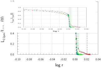
Figure 1: Model CLV profiles at ${\lambda=2.2\,\mathrm{\mu\mathrm{m}}}$ for: $\beta$ Cet (blue triangles); $\delta$ Oph (green squares); and TX Psc (red circles). The dash-dot vertical lines show the values of the impact parameter at 0.5% of the intensity: 1.008 for $\beta$ Cet, 1.013 for $\delta$ Oph, and 1.050 for TX Psc ($r$ is in Rosseland radius unit).

3.1 Computing reliable uncertainties

For each Observing Block (OB), the angular diameter is given by the modified gradient-expansion algorithm (Bevington & Robinson 1992), a robust fitting technique based on the minimisation of the weighted $\chi^{2}$, and adapted from Marquardt (1963). As “robust”, we mean a final result insensitive to small departures from the model assumptions from which the estimator is optimised (Huber & Ronchetti 2009). We improve the robustness of the results of the fitting process by removing input measurements with low SNR ($<3$), as well as values considered as extremal residuals, i.e. showing exceedingly large discrepancies with the model.

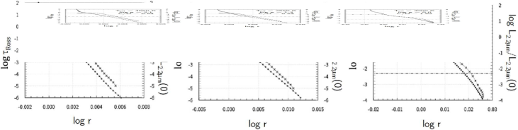
Figure 2: Rosseland optical depth (dots, left axis) and CLV profile at ${\lambda=2.2\,\mathrm{\mu\mathrm{m}}}$ (crosses, right axis) w.r.t. impact parameter (in Rosseland radius unit) for different marcs models (left and central panels: O-rich stars; right panel: C-rich). Dash-dot horizontal lines: limit of instrumental sensitivity (0.5%).

Since the data used for the fit are obtained from a complex cross-calibration process, we cannot ensure that the final uncertainties follow a Normal distribution, but the $\chi^{2}$ function remains usable as merit function for finding the best-fit model parameters. However, the formal output-parameter uncertainties, deduced from the diagonal terms of the covariance matrix of the best-fit parameters, give irrelevant and usually underestimated values (Press et al. 2007; Enders 2010). In our study, we deduce reliable uncertainties from the boundaries of the 68% confidence interval of the residual-bootstrap distribution of the best-fit angular diameters (Efron 1979, 1982; Cruzalèbes et al. 2010).

3.2 Choosing the model input parameters

Table 2 lists the stellar parameters of the science targets: effective temperature, surface gravity, and mass, of the marcs models used in the regression process, with the microturbulence parameter $\xi_{\mathrm{turb}}$=2 km s^-1. We derive these parameters from the two-dimensional B-spline interpolation of the tables of $\log T_{\mathrm{eff}}$ (de Jager & Nieuwenhuijzen 1987), $\log g$ (Allen 2001), and $\mathcal{L}/\mathcal{L}_{\odot}$ (Allen 2001), w.r.t. the spectral type.

Because this method relies on the spectral type, which carries some level of subjectivity, we concede that it is probably not the most accurate method for the determination of fundamental stellar parameters (see also the discussion in relation with Fig. 5 in Sect. 8). However, this method, currently used to measure the angular diameters of interferometric calibrators (Bordé et al. 2002; Cruzalèbes et al. 2010), provides a homogeneous way to convert various spectral types into fundamental parameters, all over the HRD. In Sect. 4, we investigate the sensitivity of the angular diameters to the adopted model stellar parameters, and show that this sensitivity is not an issue.

3.3 Fitting the model limb-darkened intensity

The spherically symmetric marcs model atmospheres, assuming local thermodynamic and hydrostatic equilibrium, are characterised by the following parameters: effective temperature $T_{\mathrm{eff}}$, surface gravity $g$, and mass $\mathcal{M}$, with ${g=G\mathcal{M}/\mathcal{R}_{\mathrm{Ross}}^{2}}$, where $\mathcal{R}_{\mathrm{Ross}}$ is the radius at ${\tau_{\mathrm{Ross}}=1}$. Using the turbospectrum code, we compute CLVs of the monochromatic radial intensity $L_{\lambda}(r)$ (also called spectral radiance, in W m^-2 $\mu$m^-1 sr^-1), where ${r=\mathcal{R}/\mathcal{R}_{\mathrm{Ross}}}$ is the impact parameter. Figure 1 shows the CLV profiles, at ${\lambda=2.2\,\mathrm{\mu\mathrm{m}}}$, calculated with turbospectrum using a marcs model, with three different sets of input parameters (Table 2), associated to : $\beta$ Cet (O-rich star, blue triangles); $\delta$ Oph (O-rich star, green squares); and TX Psc (C-rich star, red circles).

According to the Van Cittert-Zernike theorem (Goodman 1985), the monochromatic synthetic visibility of a centro-symmetric brightness distribution of angular diameter $\phi$ is

$${V}_{\lambda}\left(\phi\right)=2\pi\frac{\left|\int^{r_{\mathrm{out}}}_{0}L_{\lambda}\left(r\right)\>\mathrm{J}_{0}\left(\pi r\phi\frac{B}{\lambda}\right)\>rdr\right|}{M_{\lambda}},$$ (1)

where J₀ is the Bessel function of the first kind of order 0, $r_{\mathrm{out}}$ is the dimensionless parameter defined as ${r_{\mathrm{out}}=\mathcal{R}_{\mathrm{out}}/\mathcal{R}_{\mathrm{Ross}}}$, where $\mathcal{R}_{\mathrm{out}}$ is the outer radius, and ${M_{\lambda}=2\pi~{}{\int^{r_{\mathrm{out}}}_{0}L_{\lambda}\left(r\right)\>rdr}}$ is the monochromatic flux (also called spectral radiant exitance, in W m^-2 $\mu$m^-1). Numerical integration from 0 to $r_{\mathrm{out}}$ is performed using the trapezoidal rule on a grid, with a step width decreasing from the centre to the limb.

Figure 3: Three examples of marcs-CLV fitting results, obtained with visibility measurements: $\beta$ Cet in top panels (MJD=55 443.16); $\delta$ Oph in middle panels (MJD=54 975.24); TX Psc in bottom panels (MJD=55 143.07). Baselines are projected on the sky. The model visibility profiles at medium spectral resolution (${\mathscr{R}=1500}$) are in short dashes. The measured median absolute uncertainties in visibility are (from left to right): for $\beta$ Cet: 0.02, 0.03, and 0.02; for $\delta$ Oph: 0.010, 0.004, and 0.003; and for TX Psc: 0.015, 0.003, and 0.004.

Table 3: Sensitivity of the angular diameter $\phi$ (in mas) w.r.t. the model parameters (gravities are in c.g.s.).

	$T_{\mathrm{eff}}$ (K)	$\log~{}g=1.05$	$\log~{}g=1.9$
	3950	$\begin{cases}\phi=7.060(2)\\ \chi^{2}=2.03\end{cases}$	$\begin{cases}\phi=7.083(2)\\ \chi^{2}=1.98\end{cases}$
$\zeta$ Ara
	4250	$\begin{cases}\phi=7.039(2)\\ \chi^{2}=2.01\end{cases}$	$\begin{cases}\phi=7.066(1)\\ \chi^{2}=1.83\end{cases}$
	$T_{\mathrm{eff}}$ (K)	$\xi_{\mathrm{turb}}$=2 km s-1	$\xi_{\mathrm{turb}}$=5 km s-1
TX Psc	3000	$\begin{cases}\phi=10.053(2)\\ \chi^{2}=21.5\end{cases}$	$\begin{cases}\phi=9.986(2)\\ \chi^{2}=22.5\end{cases}$

To be accurately evaluated, the integral on $r$ in Eq.(1) requires $L_{\lambda}(r)$ to be extended all the way to a value of $r_{\mathrm{out}}$ corresponding to the lower boundary of the sensitivity of the AMBER instrument. In the $K$ band, this boundary has been measured around 0.5% of the maximum emission (Duvert et al. 2010; Absil et al. 2010). With the marcs models, the lower boundaries of the Rosseland optical depth, used to compute the intensity distributions $L_{\lambda}(r)$, are ${\tau_{\mathrm{Ross}}=10^{-6}}$ for O-rich stars, and ${\tau_{\mathrm{Ross}}=10^{-4}}$ for C-rich stars (Fig. 2). Thus, ${\mathcal{R}_{\mathrm{out}}=\mathcal{R}\left(\tau_{\mathrm{Ross}}=10^{-6}\right)}$ for O-rich stars, and ${\mathcal{R}_{\mathrm{out}}=\mathcal{R}\left(\tau_{\mathrm{Ross}}=10^{-4}\right)}$ for C-rich stars. These bottom levels ensure that the blanketing is correctly taken into account, and that the thermal structure in the line-forming region remains unchanged w.r.t. atmospheres that would be computed with even smaller optical-depth boundaries. According to Fig. 2, these optical-depth lower boundaries are associated with intensity levels of $<10^{-5}$ and $\sim 10^{-4}$, respectively, thus far below the instrumental sensitivity, as it should be to work in safe conditions. Moreover, in Sect. 4 we evaluate the sensitivity of the angular diameter to the marcs model used to compute the CLV.

Figure 3 shows three typical results of the marcs-CLV fits obtained with the visibility measurements of individual OBs, for $\beta$ Cet, $\delta$ Oph, and TX Psc. For the sake of clarity, the true visibility values are shown without error bars. In addition to the fit of the marcs-CLV profile on the true visibilities, we also compute the angular diameter using fits on triple product data (Table 4).

4 Studying the sensitivity to model parameters

The effective temperature, surface gravity and stellar mass adopted for the marcs model representing a given star are derived from the spectral type (Sect. 3.2). Unfortunately, neither the gravity, nor the stellar mass are strongly constrained by the spectral type alone. Therefore, there is a disagreement between the marcs-model parameters and the true stellar values. In this section, we study, for the 2 targets: $\zeta$ Ara (K-giant), and TX Psc (carbon star), the sensitivity of the angular diameter, to a change of input parameter values, such as: $T_{\mathrm{eff}}$, $\log g$, $\xi_{\mathrm{turb}}$.

Table 3 shows the sensitivity to the model parameters of the angular diameter, deduced from the fit on visibility data. The top table is for $\zeta$ Ara observed at MJD=54 975.36, and the bottom table is for TX Psc observed at MJD=55 143.10. The uncertainties in angular diameter are the formal 1-$\sigma$ fitting errors. The choice of the different values of $T_{\mathrm{eff}}$ and $\log g$ used for this analysis are based on the typical uncertainties, 300 K and 1 dex respectively, the latter coming from the a posteriori determination of the gravity (Sect. 8 and Fig. 7). The sensitivity to $\xi_{\mathrm{turb}}$ is studied with the values 2 and 5 km s^-1, for the carbon star.

The highest deviations from the nominal values of the angular diameter, i.e. 0.03 mas for $\zeta$ Ara and 0.07 mas for TX Psc, are smaller than the final uncertainties, 0.12 mas and 0.36 mas respectively (Table 4). Although we cannot infer quantitative general sensitivity rules from only two examples, our results show that such changes as 300 K for $T_{\mathrm{eff}}$, roughly 1 dex for $\log g$ and a factor of two for $\xi_{\mathrm{turb}}$ induce variations on the final angular diameter which are smaller than its absolute uncertainty.

5 Studying the temporal variability of the angular diameter

To study the temporal variability of the angular diameter, we group together the observing blocks of the same observing epoch over consecutive days, for each scientific target. Table 4 gives the best-fit angular diameters of the scientific targets, separately for each observation epoch and for the average over all runs. MJD is the Modified Julian Day for the middle of each observing period. The notations $\phi_{\mathrm{V}}$ and $\phi_{\mathscr{T}}$ stand for the weighted means of the angular diameters resulting from fits of the marcs CLVs on visibility and triple product data, respectively.

Figure 4 shows the temporal behaviour of the best-fit angular diameter, for our scientific targets observed over different epochs. Except for TX Psc, which shows two different values of $\phi_{\mathrm{V}}$, but not of $\phi_{\mathscr{T}}$, we find no evidence for temporal variation of the angular diameter for our targets, given the uncertainties. To perform a meaningful study of the angular-diameter time variability, a larger amount of data would have been needed for our targets. Unfortunately, we did not succeed in convincing the Observing Programmes Committee to allow supplementary observing time for this purpose.

Table 4: Best-fit angular diameters derived from the visibility and the triple product, for each observation epoch, and final angular diameters of the science targets, after averaging over all OBs. MJD is the Modified Julian Day for the middle of each observation period.

Name	MJD (days)	$\phi_{\mathrm{V}}$ (mas)	$\phi_{\mathscr{T}}$ (mas)	$\phi_{\mathrm{final}}$ (mas)
$\alpha$ Car	54 143.26	6.78(45)	6.64(1)	6.92(11)
	55 269.14	6.78(17)	6.93(2)
$\beta$ Cet	55 541.17	5.84(40)	5.45(5)	5.51(25)
$\alpha$ TrA	54 976.23	9.23(10)	9.26(8)	9.24(2)
	55 052.12	8.85(18)	9.05(5)
	55 269.32	9.34(2)	9.34(3)
$\alpha$ Hya	55 269.23	9.37(5)	9.35(7)	9.36(6)
$\zeta$ Ara	54 976.25	7.10(5)	7.09(13)	7.09(12)
	55 053.18	6.86(11)	6.98(13)
$\delta$ Oph	54 976.22	10.05(4)	9.46(7)	9.93(9)
	55 051.99	10.02(2)	9.34(2)
	55 269.88	10.43(21)	9.47(6)
$\gamma$ Hyi	55 539.80	8.77(6)	8.82(12)	8.79(9)
$o_{1}$ Ori	55 144.24	8.93(15)	10.04(5)	9.78(10)
$\sigma$ Lib	55 268.81	11.73(14)	11.19(3)	11.33(10)
$\gamma$ Ret	55 539.83	7.44(2)	7.44(2)	7.44(2)
CE Tau	55 143.28	9.94(7)	10.07(2)	9.97(8)
	55 541.24	9.94(7)	10.04(12)
T Cet	55 143.13	9.60(11)	9.70(1)	9.70(8)
TX Psc	55 143.08	9.61(21)	10.04(2)	10.23(36)
	55 541.07	10.60(6)	10.02(45)
W Ori	55 143.72	9.62(1)	9.79(7)	9.63(4)
R Scl	55 143.56	10.31(5)	9.88(2)	10.06(5)
TW Oph	54 976.35	10.59(38)	9.53(20)	9.46(30)
	55 052.19	9.19(35)	9.71(21)

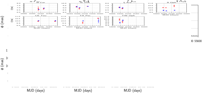
Figure 4: Temporal behaviour of the best-fit angular diameter, from visibilities (red diamonds) and triple products (blue triangles). Top panels: science targets showing no photometric variation; bottom panels: targets known as photometric variables (i.e., with a GCVS entry). The symbols which mark the results associated with the same observing epoch are slighly shifted horizontally, in order to separate the error bars.

6 Computing the final angular diameter

Rather than applying a global fit on all data sets (see e.g., Le Bouquin et al. 2008; Domiciano de Souza et al. 2008), which is the commonly used method with VLTI/AMBER data, we propose to combine multiple measurements obtained for a given star under different instrumental and environmental circumstances (see e.g., Ridgway et al. 1980; Richichi et al. 1992; Dyck et al. 1996). Using the visibility and the triple product, we compute the angular diameter averaged over all OBs, with a weighting factor derived from the uncertainty on the angular diameter, the quality of the fit, and the seeing conditions during each OB. Then, we combine the two angular-diameter values, which leads to a unique final value (last column of Table 4). We note that $\delta$ Oph is the only star for which $\phi_{\mathrm{V}}$ and $\phi_{\mathscr{T}}$ are significantly different (up to 10%, as seen in Table 4 and Fig. 4), although we have no explanation for that discrepancy.

7 Confronting our results with those of the literature

Here, we compare our final angular-diameter values with those derived from measurements obtained by other instruments or methods. Table LABEL:TabPubDiamSci gathers the values published in the literature, related to limb-darkened models, derived from indirect methods, Lunar Occultation (LO), and LBI. These values are obtained in various spectral ranges and related to various photospheric models. Their large dispersions make them difficult to use in a direct comparison with our results, which are repeated in the $\phi_{\mathrm{LBI}}$ column under Ref. (48). Therefore, we believe that the only meaningful comparison is between our values and those from the literature obtained with LBI in the same spectral domain ($K$ band), as done in the last column of Table LABEL:TabPubDiamSci.

Apart for TX Psc, only small differences are found between our new values and the published LBI values for the seven science targets: $\alpha$ Car, $\beta$ Cet, $\alpha$ Hya, $\delta$ Oph, CE Tau, W Ori, and R Scl. Such a good agreement supports the validity and the reliability of our method, which gives, in addition, reliable uncertainties. Our study provides the first LBI determinations of the angular diameter for the eight other targets: $\alpha$ TrA, $\zeta$ Ara, $\gamma$ Hyi, $o_{1}$ Ori, $\sigma$ Lib, $\gamma$ Ret, T Cet, and TW Oph.

Coming back to TX Psc, this star has often been observed in the past using high-resolution techniques, giving an angular diameter slightly larger than our new measurement. Given the error bars, our value is in good agreement with the value from Barnes et al. (1978), derived from the visual surface brightness method. Richichi et al. (1995) attribute to the temporal variability of $\phi$ already noted previously for TX Psc (a Lb-type variable) most of the disagreement between their LO measurement and the LBI values of Quirrenbach et al. (1994), obtained in the red part of the visible spectral domain with the MkIII Optical Interferometer, and of Dyck et al. (1996), obtained at 2.2 $\mu$m with the IOTA interferometer. From repeated measurements, Quirrenbach et al. suggested a substantial variation of the angular diameter, correlated with the visual magnitude, varying from 4.8 to 5.2 in 220 days (Watson et al. 2006). As shown in Sect. 5, our data tend to confirm this variation.

8 Hertzsprung – Russell Diagram

In this section, we use the values of the angular diameters of our calibrators and science targets to infer their location in the HRD ($T_{\mathrm{eff}}$ – $\mathcal{L}$).

The luminosity $\mathcal{L}$ is defined, in the marcs models, from the relation ${\mathcal{L}=4\pi\mathcal{R}_{\mathrm{Ross}}^{2}F\left(\mathcal{R}_{\mathrm{Ross}}\right)}$, where $F\left(\mathcal{R}_{\mathrm{Ross}}\right)$ is the flux per unit surface emitted by the layer located at the Rosseland radius (Gustafsson et al. 2008). The effective temperature $T_{\mathrm{eff}}$ is then defined according to ${F\left(\mathcal{R}_{\mathrm{Ross}}\right)=\sigma T_{\mathrm{eff}}^{4}}$.

We convert the best-fit angular diameter $\phi$ into an empirical Rosseland radius $\mathcal{R}_{\mathrm{obs}}$ thanks to the parallax $\varpi$. For the calibrators, $\phi$ is given by the fit of the model spectrum on the flux data. For the science targets, $\phi$ is given by the fit of the CLV profile on the SPI data. Thus, we compute the empirical luminosity $\mathcal{L}_{\mathrm{obs}}$ using the logarithmic formula

$$\log\frac{\mathcal{L}_{\mathrm{obs}}}{\mathcal{L_{\odot}}}\approx 4\log T_{\mathrm{eff}}+2\log\frac{\phi}{\varpi}-10.984(7),$$ (2)

where $T_{\mathrm{eff}}$ is in Kelvin, using the solar values $T_{\mathrm{eff},\odot}$=5777(10) K (Smalley 2005), and $\mathcal{R}_{\odot}$=0.004 6492(2) AU (Brown & Christensen-Dalsgaard 1998; Amsler et al. 2008).

Table LABEL:TabFinal gives the final fundamental parameters of our science targets and calibrators. The uncertainty-propagation formulae given by Winzer (2000), based on the second-order Taylor approximation, are used to compute the uncertainties on the derived fundamental parameters. For input uncertainties larger than 30%, we use the confidence interval transformation principle (see e.g., Smithson 2002; Kelley 2007).

To ensure consistency with the fitting process, which uses as model input parameters those derived from the spectral type (Cruzalèbes et al. 2013 and Table 2), the value adopted for the effective temperature of the star is the value listed in Table 2.

To assess the accuracy of the value, we compare the effective temperature deduced from the spectral type for the giants and supergiants of types K and M, included in our samples of science and calibrator targets, with the temperature derived from the de-reddened $V-K$ index, using the empirical relationship provided by van Belle et al. (1999)

$$T_{\mathrm{eff}}~{}\mathrm{(K)}\ =\ 3030+4750\times 10^{-0.187\left(V-K\right)},$$ (3)

where $2<V-K<9$. We find that the agreement between the effective temperatures, shown in Fig. 5, is quite satisfactory, since their discrepancy is less than $\pm$300 K, which is of the same order than the absolute uncertainty given by the van Belle’s formula ($\pm$250 K). For the three carbon stars W Ori, R Scl, and TW Oph, the adopted effective temperature of 2600 K (Table 2) is consistent with the values derived by Lambert et al. (1986) with $\pm$100 K uncertainty: respectively 2680 K, 2550 K, and 2450 K.

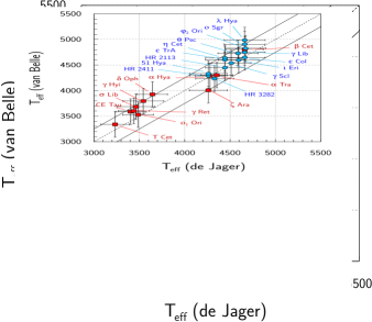
Figure 5: Effective temperatures deduced from the de-reddened $V-K$ color index (van Belle), versus from the spectral type (de Jager), for the targets of our observing sample. Red squares: science targets. Blue dots: calibrators. Solid lines: $\pm$250 K thresholds.

Figure 6 shows the resulting $T_{\mathrm{eff}}$ – $\mathcal{L}_{\mathrm{obs}}$ diagram, including the calibrators and the science targets. In order to distinguish between the error bars, the data points for R Scl, W Ori and TW Oph are slightly shifted horizontally, although these 3 carbon stars have the same effective temperature 2600 K. This HRD displays as well evolutionary tracks from the Padova set (Bertelli et al. 2008, 2009), for ${Y=0.26}$ and ${Z=0.017}$, and for masses between 1 and 8 $\mathcal{M}_{\odot}$, where $Y$ is the helium abundance, and $Z$ the metallicity.

These tracks make it possible to derive a rough estimate of the stellar mass $\mathcal{M}$, thus of the gravity $g_{\mathrm{obs}}$ at the Rosseland surface, deduced from the relation

$$\log g_{\mathrm{obs}}\approx\log\frac{\mathcal{M}}{\mathcal{M}_{\odot}}-2\log\frac{\mathcal{R}_{\mathrm{obs}}}{\mathcal{R}_{\odot}}+4.4374(5),$$ (4)

using the value of the solar surface gravity given by Gray (2005). These mass and gravity values are also included in Table LABEL:TabFinal. The comparison of the surface gravities $\log~{}g$, deduced from the spectral type and used to select the marcs models, with those derived a posteriori from the HRD, is done in Figure 7. We see that they agree within $\pm 0.5$ dex, except for the calibrator $\alpha$ Ret (${\log g-\log g_{\mathrm{obs}}=-0.80}$), and for the science targets $\alpha$ Car (+0.82), and $\zeta$ Ara (+0.67). Since the determination of the mass from the position along the evolutionary tracks in the HRD is well-constrained, we attribute the discrepancy in surface gravity to the ill-defined value derived from the spectral type and used for the model, at least for these 3 targets.

With the linear radius derived from the interferometry, and the luminosity following the relationship ${\mathcal{L}=4\pi\mathcal{R}^{2}\sigma T_{\mathrm{eff}}^{4}}$, the location of our targets in the HRD allows us to perform interesting checks of stellar structure related to the presence or absence of technetium, and to the Period – Luminosity relationship.

9 Technetium

Technetium is an s-process element with no stable isotope that was first identified in the spectra of some M and S stars by Merrill (1952). With a laboratory half-life of $2.13\times 10^{5}$ yr, the technetium isotope ⁹⁹Tc is the only one produced by the s-process in thermally-pulsating AGB (TP-AGB) stars (see Goriely & Mowlavi 2000). Due to the existence of an isomeric state of the ⁹⁹Tc nucleus, the high temperatures encountered during thermal pulses strongly shorten the effective half-life of ⁹⁹Tc ($t_{1/2}\sim$ 1 yr at $\sim 3\times 10^{8}$ K) (Cosner et al. 1984), but the large neutron densities delivered by the ²²Ne($\alpha$,n)²⁵Mg neutron source, operating at these high temperatures, more than compensate the reduction of the ⁹⁹Tc lifetime (Mathews et al. 1986), and enable a substantial technetium production. The dredge-up episodes then carry technetium to the envelope, where it decays steadily at its terrestrial rate of $t_{1/2}$=$2.13\times 10^{5}$ yr. Starting from an abundance associated with the maximum observed in Tc-rich AGB stars, technetium should remain detectable during 1.0 to $1.5\times 10^{6}$ yr (Smith & Lambert 1988). If the dredge-up of heavy elements occurs after each thermal pulse, occurring every 0.1 to $0.3\times 10^{6}$ yr, virtually all s-process enriched TP-AGB stars should exhibit technetium lines.

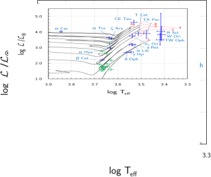
Figure 6: $T_{\mathrm{eff}}$ – $\mathcal{L}_{\mathrm{obs}}$ diagram of the calibrators (thin green error bars) and science targets (thick blue error bars), with evolutionary tracks (black full lines) and asymptotic giant branches (red dashed lines), for different masses, indicated in red at the end of each track.

This conclusion applies to the situation where the s-process is powered by the ²²Ne($\alpha$,n)²⁵Mg neutron source operating in the thermal pulse itself. However, Straniero et al. (1995) advocated that the s-process nucleosynthesis mainly occurs during the interpulse with neutrons from ¹³C($\alpha$,n)¹⁶O (see Käppeler et al. 2011, for a recent review). When this process occurs in low-mass stars, and technetium is engulfed in the subsequent thermal pulse, it should not decay at a fast rate, because the arguments put forward by Cosner et al. (1984) and Mathews et al. (1986), and discussed above, only apply to intermediate-mass stars with hot thermal pulses.

One thus reaches the conclusion that s-process-enriched TP-AGB stars, of both low and intermediate mass, should necessarily exhibit technetium, unless the time span between successive dredge-ups become comparable to the Tc lifetime in the envelope. Indeed, all the S stars identified as TP-AGB stars by Van Eck et al. (1998) thanks to the Hipparcos parallaxes turned out to be Tc-rich, and a survey of technetium in the large Henize sample of S stars did not challenge that conclusion either (Van Eck & Jorissen 1999, 2000).

The present sample allows us to check whether a similar conclusion holds true for a sample comprising oxygen-rich giants and supergiants, as well as carbon stars. The technetium content of our science targets has been collected from the literature (last column of Table LABEL:TabObsSci), and displayed in graphical form in Fig. 8 where it is confronted to the TP-AGB tracks (dashed lines) for different stellar masses. The presence or absence of Tc conforms to the expectations that namely TP-AGB stars exhibit Tc, except for the carbon star W Ori, where Tc has been tagged as absent by two independent studies, despite the fact that this star lies well within the TP-AGB region, as it should for a cool carbon star anyway. The s-process content of that star has been studied by Abia et al. (2002) who find only moderate s-process enhancements, if any ($\leq 0.3$ dex), and this fact alone may explain the absence of detectable Tc. With the stellar parameters now available from our interferometric study for two more carbon stars (R Scl and TW Oph) falling in that region of the HRD, it will be of interest to perform a similar analysis on these two stars to get constraints on their nucleosynthesis processes.

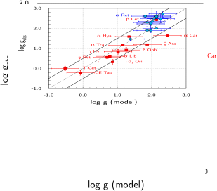
Figure 7: Comparison of the surface gravities used to select the marcs models, with the values $\log g_{\mathrm{obs}}$ derived from our final angular-diameter value. Red squares: science targets; blue dots: calibrators. The solid lines mark the $\pm 0.5$ dex thresholds.

10 Period – Luminosity relation

Since the present study derives radii and masses for some semi-regular variables, we also derive the pulsation constant $Q$ (e.g., Fox & Wood 1982), defined as

$$Q=P\;\left(\frac{\mathcal{M}}{\mathcal{M}_{\odot}}\right)^{1/2}\;\left(\frac{\mathcal{R}_{\mathrm{obs}}}{\mathcal{R}_{\odot}}\right)^{-3/2},$$ (5)

where $P$ is the pulsation period given in Table LABEL:TabObsSci. For pulsating stars with available periods of variation, we include $Q$ in Table LABEL:TabFinal (last column). Values of $Q$ smaller than 0.04 d are typical of overtone pulsators (Fox & Wood 1982). Indeed, in the Period – Luminosity diagram ($M_{\mathrm{K}},P$) shown in Fig. 9, and following the terminology introduced by Wood (2000), most of these stars fall on the A’, A and B overtone sequences, whilst only a few (TW Oph, TX Psc and R Scl) fall on the Mira fundamental-mode sequence C, despite the fact that these smaller-amplitude carbon stars are actually classified as semi-regulars.

We note that masses should increase along each sequence, as predicted by theory (e.g., Fig. 8 of Wood 1990). This is indeed the case, with our observed sample, with the exception of W Ori (${\mathcal{M}=1.5\mathcal{M}_{\odot}}$) and T Cet (${\mathcal{M}=3\mathcal{M}_{\odot}}$) along sequence B. Taking into account the large uncertainty of its bolometric magnitude ${M_{\mathrm{bol}}=-5(1)}$, derived from its absolute luminosity (Table LABEL:TabFinal), the location of the C-rich star W Ori on sequence B is rather uncertain. Using instead ${M_{\mathrm{bol}}=-4}$ eliminates the problem, since it moves W Ori to its right position along sequence C, where the three other carbon stars of our sample are located.

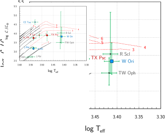
Figure 8: Same as Fig. 6 restricted to the science targets, with their technetium content indicated. Large red circles: Tc present; small red circle: Tc probably present; large blue squares: Tc absent; small blue square: Tc doubtful; small black dots: unknown Tc content. Red dashed lines: TP-AGB tracks, for masses indicated at the end of each curve.

11 Conclusion

We present new determinations of the angular diameter of a set of ten O-rich giants, two supergiants, and four C-rich giants, observed in the $K$-band (${\mathscr{R}=1500}$) during several runs of a few nights, distributed over two years, using the VLTI/AMBER facility. They are obtained from the fit of synthetic SPectro-Interferometric (SPI) visibility and triple product on the true data. The synthetic SPI observables are derived by using CLV profile calculated from marcs model atmospheres.

We show that the results are moderately impacted ($<$ 1% in angular diameter) by the variation of the model input parameters T_eff, $\log g$, and $\xi_{\mathrm{turb}}$. During the observing period, using configurations covering different baseline angles, we find no significant variation of the angular diameter, except for TX Psc, a result which needs to be confirmed with complementary observations. For the eight targets previously measured by LBI in the same spectral band, our new angular-diameter values are in good agreement with those of the literature. Except for TX Psc, the relative deviations between our values and those of the literature are less than 5%, which validates our method. For TX Psc, a substantial temporal variation of the angular diameter, suspected to be correlated with the visual magnitude, could be invoked to account for the larger discrepancy. For the eight other targets, our values are first determinations, since no angular-diameter measurement have been published yet for these stars.

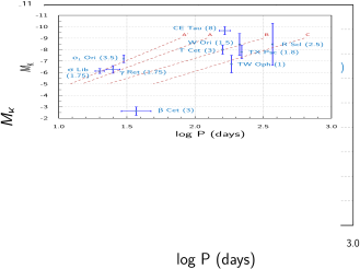
Figure 9: Period – Luminosity diagram for science targets with available pulsation periods. $M_{\mathrm{K}}$ values are derived from the dereddened K magnitudes and the distance moduli. Stellar masses between parentheses (in $\mathcal{M}_{\odot}$). Location of A’ to C sequences taken from Tabur et al. (2010).

These angular diameters are used to place the stars in the Hertzsprung-Russell Diagram (HRD) and to derive their masses. For stars with a known technetium content, we confront their location in the HRD to the prediction that s-process nucleosynthesis producing technetium operates in thermally-pulsing AGB (TP-AGB) stars. The two Tc-rich stars ($o_{1}$ Ori and TX Psc) indeed fall along the TP-AGB, as expected. But the low-mass carbon-rich star W Ori, despite being located close to the top of the low-mass TP-AGB, has been flagged as devoid of Tc, which, if confirmed, would put interesting constraints on the s-process in low-mass carbon stars.

Finally, we compute the pulsation constant for the pulsating stars with available periods of variation. Their location along the pulsation sequences in the Period – Luminosity diagram confirms the mass dependency predicted by the theory, except for W Ori and T Cet.

Those results, based on measurements of visibilities and triple products, illustrate the several ways to include LBI observations in the general investigation process in the field of stellar astrophysics.

Table 1: Relevant observational parameters of the observed sample of science targets.

Name	Spec. type	$\varpi_{\mathrm{Hip}}$a	$m_{\mathrm{K}}$b	$m_{V}$c	$A_{V}$d	$(V-K)_{0}$	Compo.e	Sep.e	PAe	$\Delta V$e	Var. typec	Periodc	Tcg	Calibh
		(mas)						(″)	(°)			(days)
$\alpha$ Car	F0II8	10.6(6)	-1.3(3)	-0.62(5)	0.07(15)	0.6(3)	-	-	-	-	-	-	unkn.	$\eta$ Col
$\beta$ Cet	K0III13	33.9(2)	-0.3(4)	1.96-2.11	0.03(19)	2.3(4)	-	-	-	-	SRB17	37(4)17	unkn.	$\eta$ Cet
$\alpha$ TrA	K2II14	8.4(2)	-1.2(1)	1.91(5)	0.08(15)	3.1(2)	-	-	-	-	-	-	unkn.	$\varepsilon$ TrA
$\alpha$ Hya	K3II-III2	18.1(2)	-1.1(2)	1.93-2.01	0.03(14)	3.1(3)	AB	283	153	8	Susp.	-	unkn.	$\lambda$ Hya
							AC	210	90	-	-	-	unkn.
$\zeta$ Ara	K3III3	6.7(2)	-0.6(2)	3.12(5)	0.07(15)	3.7(3)	-	-	-	-	-	-	unkn.	$\varepsilon$ TrA/o Sgr
$\delta$ Oph	M0.5III2	19.1(2)	-1.2(2)	2.72-2.75	0.03(15)	3.9(3)	AB	66	294	9	Susp.	-	unkn.	$\gamma$ Lib/$\varepsilon$ TrA
$\gamma$ Hyi	M2III1	15.2(1)	-1.0(4)	3.32-3.38	0.04(16)	4.2(5)	-	-	-	-	SRB	-	unkn.	$\alpha$ Ret
$o_{1}$ Ori	M3III5	5.0(7)	-0.7(2)	4.65-4.88	0.16(17)	5.2(2)	AB7	-	-	11.7	SRB	30(1)	yes6,11	HR 2411
$\sigma$ Lib	M3.5III4	11.3(3)	-1.4(2)	3.20-3.46	0.03(14)	4.6(3)	-	-	-	-	SRB	20(1)	no6,11	51 Hya/$\varepsilon$ TrA
$\gamma$ Ret	M4III3	7.0(1)	-0.5(3)	4.42-4.64	0.08(15)	4.9(4)	AB	0.2	-	-	SR	25(1)	unkn.	$\alpha$ Ret
CE Tau	M2Iab-b3	1.8(3)	-0.9(2)	4.23-4.54	0.29(19)	5.0(3)	-	-	-	-	SRC	165(1)	doubt.6	$\phi_{2}$ Ori
T Cet	M5.5Ib/II8	3.7(5)	-0.8(3)	4.96-6.9	0.08(19)	6.4(3)	-	-	-	-	SRC	159.3(1)	prob.6	$\iota$ Eri/$\gamma$ Scl
TX Psc	C7,2(N0)(Tc)10	3.6(4)	-0.5(3)	4.79-5.20	0.11(10)	5.4(3)	-	-	-	-	LB	220(1)9	yes6,16	$\theta$ Psc
W Ori	C5,4(N5)10	2.6(10)15	-0.5(4)	5.5-6.9	0.11(15)	6.4(5)	-	-	-	-	SRB	212(1)	no12,16	$\phi_{2}$ Ori/HR 2113
R Scl	C6,5ea(Np)10	2.1(15)15	-0.1(1)	9.1-12.9	0.11(10)	6.6(2)	ABf	10	234	12	SRB	370(1)	unkn.	$\iota$ Eri
TW Oph	C5,5(Nb)10	3.7(12)15	0.5(4)	11.6-13.8	0.10(16)	7.0(4)	-	-	-	-	SRB	185(1)	unkn.	o Sgr/$\gamma$ Lib

¹Landi Dessy & Keenan (1966); ²Morgan & Keenan (1973); ³Houk & Cowley (1975); ⁴Houk (1978); ⁵Smith & Lambert (1985); ⁶Little et al. (1987); ⁷Ake & Johnson (1988); ⁸Houk & Smith-Moore (1988); ⁹Wasatonic (1997); ¹⁰Kholopov et al. (1998); ¹¹Lebzelter & Hron (1999); ¹²Abia et al. (2001); ¹³Montes et al. (2001); ¹⁴Bordé et al. (2002); ¹⁵Knapp et al. (2003); ¹⁶Lebzelter & Hron (2003); ¹⁷Otero & Moon (2006)

^aunless quoted, from the New HIPPARCOS Astrometric Catalogue (van Leeuwen 2007)
^bfrom the 2MASS Catalogue (Skrutskie et al. 2006)
^cmagnitude variations, variability type, and period of variability taken (unless quoted) from the AAVSO-VSX Database (Watson et al. 2006). “Susp.” stands for suspected variability
^dcalculated thanks the numerical algorithm of Hakkila et al. (1997), including the studies of Fitzgerald (1968), Neckel & Klare (1980), Berdnikov & Pavlovskaya (1991), Arenou et al. (1992), Chen et al. (1998), and Drimmel & Spergel (2001), plus a sample of studies of high-galactic latitude clouds
^emultiplicity parameters from the WDS Catalogue (Mason et al. 2001)
^fthe A component is seen double by Maercker et al. (2012) with ALMA
^gqualitative information on the technetium content (unkn. stands for “unknown”, doubt. for “doubtful”, and prob. for “probable”)
^hassociated calibrator(s), with angular diameter given by Cruzalèbes et al. (2013)

Table 5: Published angular diameters (in mas) of the scientific targets. We note $\phi_{\mathrm{ind}}$ the angular diameter derived from indirect methods, while we note $\phi_{\mathrm{LO}}$ and $\phi_{\mathrm{LBI}}$ the limb-darkened angular diameters derived from Lunar Occultation and Long-Baseline Interferometry measurements, respectively. The values in bold are the averaged values, using weights inversely proportional to the uncertainties. When not quoted, conservative 10% errors are adopted. “Ref.” stands for the bibliographical reference from which each value is taken, as listed at the end of the Table, and “Diff.” stands for the relative difference between our new measurement and the averaged published LBI values obtained with a similar instrumental configuration. Our values are included in the $\phi_{\mathrm{LBI}}$ column under Ref. (48).

Name	$\phi_{\mathrm{ind}}$	Ref.	$\phi_{\mathrm{LO}}$	Ref.	$\phi_{\mathrm{LBI}}$	Ref.	Diff.
$\alpha$ Car	5.9(4)	16			6.6(8)	5
	6.0(7)	3			6.86(41)	2
	6.5(8)	11			6.92(11)	48	-0.1%
	6.8(4)	13			6.93(15)	42
	7.1(2)	9
	7.22(42)	37
	6.7				6.9
$\beta$ Cet	5.03(40)	19			5.29(8)	46
	5.31(6)	35			5.329(5)	44
	5.4(8)	16			5.51(25)	48	+3.4%
	5.66(39)	45
	6.5	24
	7.4(9)	3
	8.0	20
	5.6				5.3
$\alpha$ TrA	11.6(17)	16			9.24(2)	48
	8.98(10)	35
	9.81(39)	40
	15.0(18)	3
	9.5
$\alpha$ Hya	9.30(39)	9			9.73(10)	38
	9.4(9)	23			9.335(16)	44
	9.9(10)	13			9.36(6)	48	+0.3%
	10.0(15)	16
	14.0(17)	3
	10.0				9.4
$\zeta$ Ara	7.21(21)	39			7.09(12)	48
	7.2	20
	7.6(11)	16
	7.62(53)	45
	9.0	24
	11.0(13)	3
	7.6
$\delta$ Oph	10(1)	21			9.50(50)	30
	10.03(10)	35			9.93(9)	48	+2.1%
	10.18(20)	25			9.946(13)	44
	10.22(71)	45			10.47(12)	38
	10.23(31)	40
	11.6(17)	16
	11.0	24
	13	1
	13.0(16)	3
	26(7)	8
	10.4				10.0
$\gamma$ Hyi	9.5	33			8.79(9)	48
	9.8(15)	16
	10.0(12)	3
	9.7
$o_{1}$ Ori	7.1(21)	3			9.78(10)	48
$\sigma$ Lib	11.0(13)	3			11.33(10)	48
	12.05(83)	45
	12.5	20
	13.0	24
	12.1
$\gamma$ Ret	7.5(2)	32			7.44(2)	48
	8.0	33
	11.0(33)	16
	7.8
CE Tau	9.4(11)	3	9.1(8)	15	9.3(5)	34
	13	1	10.9(10)	14	9.83(7)	30
	13.0(20)	16	17(1)	18	9.97(8)	48	+3.7%
					10.68(21)	27
	11.5		12.1		10.0
T Cet	13.1(39)	16			9.70(8)	48
	14.5	43
	14.1
TX Psc	6.2	12	8.40(5)	29	10.23(36)	48	-10.6%
	9.5(5)	11	8.9(10)	4	11.2(10)	28
			9.31(75)	10	11.44(30)	31
			10(3)	6
			10.2(25)	7
	8.0		8.5		10.9
W Ori					9.63(4)	48	-2.8%
					9.91(60)	31
					9.7
R Scl	12.2	22			10.06(5)	48	-1.4%
	12.0	26			10.2(5)	47
	12.1	41
	12.75(98)	36
	12.3				10.1
TW Oph			10.4(5)	17	9.46(30)	48

Table 5: continued.

(1) Hertzsprung (1922); (2) Hanbury Brown et al. (1967); (3) Wesselink et al. (1972); (4) de Vegt (1974); (5) Hanbury Brown et al. (1974); (6) Morbey & Fletcher (1974); (7) Dunham et al. (1975); (8) Currie et al. (1976); (9) Blackwell & Shallis (1977); (10) Ridgway et al. (1977); (11) Barnes et al. (1978); (12) Scargle & Strecker (1979); (13) Blackwell et al. (1980); (14) White (1980); (15) Beavers et al. (1982); (16) Ochsenbein & Halbwachs (1982); (17) Ridgway et al. (1982); (18) White et al. (1982); (19) Eriksson et al. (1983); (20) Johnson & Wright (1983); (21) Leggett et al. (1986); (22) Rowan-Robinson et al. (1986); (23) Bell & Gustafsson (1989); (24) Slee et al. (1989); (25) Blackwell et al. (1990); (26) Judge & Stencel (1991); (27) Quirrenbach et al. (1993); (28) Quirrenbach et al. (1994); (29) Richichi et al. (1995); (30) Dyck et al. (1996); (31) Dyck et al. (1996); (32) Bedding et al. (1997); (33) Dumm & Schild (1998); (34) Dyck et al. (1998); (35) Cohen et al. (1999); (36) Yudin & Evans (2002); (37) Decin et al. (2003); (38) Mozurkewich et al. (2003); (39) Ohnaka et al (2005); (40) Engelke et al. (2006); (41) Dehaes et al. (2007); (42) Domiciano de Souza et al. (2008); (43) Ramstedt et al. (2009); (44) Richichi et al. (2009); (45) Lafrasse et al. (2010); (46) Berio et al. (2011); (47) Sacuto et al. (2011); (48) present work

Table 6: Final values of the stellar fundamental parameters (top part: science targets; bottom part: calibrators).

Name	$\mathcal{R}_{\mathrm{obs}}$/$\mathcal{R}_{\odot}$a	$\log T_{\mathrm{eff}}$b	$\log\mathcal{L}_{\mathrm{obs}}$/$\mathcal{L}_{\odot}$c	$M_{\mathrm{bol}}$d	$\mathcal{M}$/$\mathcal{M}_{\odot}$e	$\log g_{\mathrm{obs}}$f	$Q$g
$\alpha$ Car	71(4)	3.845(6)	4.03(5)	-5.34(13)	8.0(3)	1.64(5)	-
$\beta$ Cet	17.5(9)	3.668(9)	2.21(6)	-0.54(14)	3.0(3)	2.43(6)	0.879(121)
$\alpha$ TrA	119(2)	3.638(10)	3.66(4)	-4.41(11)	7-8	1.16(3)	-
$\alpha$ Hya	55.7(7)	3.633(10)	2.98(4)	-2.71(10)	4-5	1.60(5)	-
$\zeta$ Ara	114(4)	3.628(10)	3.58(5)	-4.21(12)	7-8	1.20(4)	-
$\delta$ Oph	56.0(7)	3.562(12)	2.70(5)	-2.01(12)	1.0(3)	0.93(12)	-
$\gamma$ Hyi	62(1)	3.544(12)	2.71(5)	-2.05(13)	1.0(3)	0.84(12)	-
$o_{1}$ Ori	214(29)	3.538(13)	3.76(13)	-4.65(31)	3-4	0.32(13)	0.019(4)
$\sigma$ Lib	108(3)	3.538(13)	3.17(5)	-3.18(14)	1.5-2	0.61(7)	0.024(2)
$\gamma$ Ret	115(2)	3.538(13)	3.23(5)	-3.33(13)	1.5-2	0.55(6)	0.027(2)
CE Tau	601(83)	3.531(13)	4.63(13)	-6.83(32)	8.0(3)	-0.21(12)	0.033(7)
T Cet	275(34)	3.531(13)	3.91(12)	-5.03(30)	3.0(3)	0.01(11)	0.059(11)
TX Psc	293(66)	3.512(13)	3.90$\left({}^{21}_{31}\right)$	-5.02(61)	1.8(3)	-0.30(21)	0.056(17)
W Ori	406(185)	3.415(17)	3.83$\left({}^{51}_{37}\right)$	-4.85(103)	1-2	-0.60$\left({}^{42}_{63}\right)$	0.032$\left({}^{30}_{20}\right)$
R Scl	513(721)	3.415(17)	4.04$\left({}^{117}_{55}\right)$	-5.35(201)	2-3	-0.59(75)	0.050$\left({}^{76}_{44}\right)$
TW Oph	278(102)	3.415(17)	3.50$\left({}^{42}_{34}\right)$	-4.02(89)	1.0(3)	-0.46$\left({}^{38}_{47}\right)$	0.040$\left({}^{32}_{21}\right)$
$\alpha$ Ret	13.5(3)	3.679(9)	1.93(4)	-0.10(11)	2.5-3	2.61(5)	-
$\varphi_{2}$ Ori	8.8(1)	3.669(9)	1.52(4)	0.95(10)	1-2	2.73$\left({}^{13}_{19}\right)$	-
$\eta$ Col	37.1(12)	3.668(9)	2.77(5)	-2.17(12)	5.0(3)	2.00(4)	-
$\lambda$ Hya	9.7(8)	3.668(9)	1.60(8)	0.74(20)	1-2	2.64$\left({}^{20}_{25}\right)$	-
$\gamma$ Lib	12.4(6)	3.668(9)	1.81(6)	0.21(14)	2.0(3)	2.55(7)	-
$o$ Sgr	11.7(9)	3.668(9)	1.76(7)	0.33(19)	2.0(3)	2.60(8)	-
$\iota$ Eri	11.7(10)	3.663(9)	1.74(8)	0.40(21)	1-2	2.48$\left({}^{20}_{25}\right)$	-
$\theta$ Psc	10.4(7)	3.662(9)	1.63(7)	0.67(17)	1-1.5	2.50(14)	-
$\gamma$ Scl	12.3(1)	3.654(10)	1.75(4)	0.37(10)	1-1.5	2.35(10)	-
HR 2113	35(4)	3.647(10)	2.62(10)	-1.82(24)	3-4	1.90(11)	-
$\varepsilon$ TrA	16.2(2)	3.647(10)	1.96(4)	-0.16(10)	1-2	2.20$\left({}^{14}_{19}\right)$	-
$\eta$ Cet	13.6(1)	3.647(10)	1.81(4)	0.22(10)	1-1.5	2.26(9)	-
HR 3282	78(6)	3.636(10)	3.28(8)	-3.45(20)	6-7	1.47(8)	-
HR 2411	22.7(10)	3.629(10)	2.18(6)	-0.72(14)	1-2	1.90$\left({}^{16}_{21}\right)$	-
51 Hya	11.6(6)	3.629(10)	1.60(6)	0.74(16)	1.0(3)	2.30(12)	-

^aRosseland radius derived from the angular diameter $\phi$ and the parallax $\varpi$
^beffective temperature of the model (in K)
^cempirical stellar luminosity, derived from Eq. (2)
^dbolometric magnitude derived from the stellar luminosity
^estellar mass derived from the position along the evolutionary track in the HRD. If two tracks with different masses pass through the star location, two possible mass values are listed
^fsurface gravity, derived from Eq. (4)
^gpulsation constant (in days), derived from Eq. (5)

References

- Abia et al. (2001) Abia C., Busso M., Gallino R., Domínguez I., Straniero O., Isern J., 2001, ApJL, 559, 1117
- Abia et al. (2002) Abia C. et al., 2002, ApJL, 579, 817
- Absil et al. (2010) Absil O. et al., 2010, A&A, 520, L2
- Ake & Johnson (1988) Ake T. B., Johnson H. R., 1988, ApJ, 327, 214
- Allen (2001) Allen C. W., 2001, Allen’s Astrophysical Quantities, 4th edn. Springer-Verlag, New York, NY
- Alvarez & Plez (1998) Alvarez R., Plez B., 1998, A&A, 330, 1109
- Amsler et al. (2008) Amsler C. et al., 2008, Phys. Lett. B, 667
- Arenou et al. (1992) Arenou F., Grenon M., Gomez A., 1992, A&A, 258, 104
- Barnes et al. (1978) Barnes T. G., Evans D. S., Moffett T. J., 1978, MNRAS, 183, 285
- Baschek et al. (1991) Baschek B., Scholz M., Wehrse R., 1991, A&A, 246, 374
- Bastian & Hefele (2005) Bastian U., Hefele H., 2005, in C. Turon, K. S. O’Flaherty, & M. A. C. Perryman ed., The Three-Dimensional Universe with Gaia Vol. 576 of ESA Special Publ. Astrometric Limits Set by Surface Structure, Binarity, Microlensing. ESA, Noordwijk, The Netherlands, pp 215–221
- Beavers et al. (1982) Beavers W. I., Cadmus R. R., Eitter J. J., 1982, AJ, 87, 818
- Bedding et al. (1997) Bedding T. R., Zijlstra A. A., von der Luhe O., Robertson J. G., Marson R. G., Barton J. R., Carter B. S., 1997, MNRAS, 286, 957
- Bell & Gustafsson (1989) Bell R. A., Gustafsson B., 1989, MNRAS, 236, 653
- Berdnikov & Pavlovskaya (1991) Berdnikov L. N., Pavlovskaya E. D., 1991, SvA, 17, 215
- Berio et al. (2011) Berio P. et al., 2011, A&A, 535, A59
- Bertelli et al. (2008) Bertelli G., Girardi L., Marigo P., Nasi E., 2008, A&A, 484, 815
- Bertelli et al. (2009) Bertelli G., Nasi E., Girardi L., Marigo P., 2009, A&A, 508, 355
- Bevington & Robinson (1992) Bevington P. R., Robinson D. K., 1992, Data Reduction and Error Analysis for The Physical Sciences. McGraw-Hill, New York, NY
- Blackwell et al. (1990) Blackwell D. E., Petford A. D., Arribas S., Haddock D. J., Selby M. J., 1990, A&A, 232, 396
- Blackwell et al. (1980) Blackwell D. E., Petford A. D., Shallis M. J., 1980, A&A, 82, 249
- Blackwell & Shallis (1977) Blackwell D. E., Shallis M. J., 1977, MNRAS, 180, 177
- Bonneau et al. (2006) Bonneau D. et al., 2006, A&A, 456, 789
- Bordé et al. (2002) Bordé P., Coudé du Foresto V., Chagnon G., Perrin G., 2002, A&A, 393, 183
- Brown & Christensen-Dalsgaard (1998) Brown T. M., Christensen-Dalsgaard J., 1998, ApJL, 500, L195
- Chen et al. (1998) Chen B., Vergely J. L., Valette B., Carraro G., 1998, A&A, 336, 137
- Chiavassa et al. (2011) Chiavassa A. et al., 2011, A&A, 528, A120
- Cohen et al. (1999) Cohen M., Walker R. G., Carter B., Hammersley P., Kidger M., Noguchi K., 1999, AJ, 117, 1864
- Cosner et al. (1984) Cosner K. R., Despain K. H., Truran J. W., 1984, ApJL, 283, 313
- Cruzalèbes et al. (2010) Cruzalèbes P., Jorissen A., Sacuto S., Bonneau D., 2010, A&A, 515, A6
- Cruzalèbes et al. (2013) Cruzalèbes P. et al., 2013, accepted for publication in MNRAS, preprint (arXiv:1304.1666)
- Cruzalèbes et al. (2008) Cruzalèbes P., Spang A., Sacuto S., 2008, in Kaufer A., Kerber F., eds, The 2007 ESO Instrument Calibration Workshop Calibration of AMBER Visibilities at Low Spectral Resolution. Springer-Verlag, Berlin Heidelberg, Germany, pp 479–482
- Currie et al. (1976) Currie D. G., Knapp S. L., Liewer K. M., Braunstein R. H., 1976, Tech. Rep. 76-125, Stellar disk diameter measurements by amplitude interferometry 1972-1976. Dept Phys. Astron., Univ. Maryland
- de Jager & Nieuwenhuijzen (1987) de Jager C., Nieuwenhuijzen H., 1987, A&A, 177, 217
- de Vegt (1974) de Vegt C., 1974, A&A, 34, 457
- Decin et al. (2003) Decin L., Vandenbussche B., Waelkens K., Eriksson C., Gustafsson B., Plez B., Sauval A. J., 2003, A&A, 400, 695
- Dehaes et al. (2007) Dehaes S., Groenewegen M. A. T., Decin L., Hony S., Raskin G., Blommaert J. A. D. L., 2007, MNRAS, 377, 931
- Delfosse (2004) Delfosse X., 2004, Technical report, Stellar diameter estimation from photospheric indices. JMMC, Grenoble, France
- Domiciano de Souza et al. (2008) Domiciano de Souza A., Bendjoya P., Vakili F., Millour F., Petrov R. G., 2008, A&A, 489, L5
- Drimmel & Spergel (2001) Drimmel R., Spergel D. N., 2001, ApJL, 556, 181
- Dumm & Schild (1998) Dumm T., Schild H., 1998, NewA, 3, 137
- Dunham et al. (1975) Dunham D. W., Evans D. S., Silverberg E. C., Wiant J. R., 1975, MNRAS, 173, 61P
- Duvert et al. (2010) Duvert G., Chelli A., Malbet F., Kern P., 2010, A&A, 509, A66
- Dyck et al. (1996) Dyck H. M., Benson J. A., van Belle G. T., Ridgway S. T., 1996, AJ, 111, 1705
- Dyck et al. (1996) Dyck H. M., van Belle G. T., Benson J. A., 1996, AJ, 112, 294
- Dyck et al. (1998) Dyck H. M., van Belle G. T., Thompson R. R., 1998, AJ, 116, 981
- Efron (1979) Efron B., 1979, Ann. Statist., 7, 1
- Efron (1982) Efron B., 1982, The Jacknife, the Bootstrap, and other Resampling Plans. No. 38 in Reg. Conf. Ser. in Appl. Math. SIAM-NF-CBMS, Philadelphia, PA
- Enders (2010) Enders G. K., 2010, Applied missing data analysis. Methodol. Social Sci. Ser. Guilford Press, New York, NY
- Engelke et al. (2006) Engelke C. W., Price S. D., Kraemer K. E., 2006, AJ, 132, 1445
- Eriksson et al. (1983) Eriksson K., Linsky J. L., Simon T., 1983, ApJL, 272, 665
- Eriksson & Lindegren (2007) Eriksson U., Lindegren L., 2007, A&A, 476, 1389
- Fitzgerald (1968) Fitzgerald M. P., 1968, AJ, 73, 983
- Fox & Wood (1982) Fox M. W., Wood P. R., 1982, ApJL, 259, 198
- Gai et al. (2004) Gai M. et al., 2004, in W. A. Traub ed., New Frontiers in Stellar Interferometry Vol. 5491 of SPIE Conf. Ser., The VLTI fringe sensors: FINITO and PRIMA FSU. SPIE, Bellingham, WA, pp 528–539
- Goodman (1985) Goodman J. W., 1985, Statistical Optics. Wiley Classics Libr., New York, NY
- Goriely & Mowlavi (2000) Goriely S., Mowlavi N., 2000, A&A, 362, 599
- Gray (2005) Gray D. F., 2005, The Observation and Analysis of Stellar Photospheres, 3rd edn. Cambridge Univ. Press, Cambridge, UK
- Gustafsson et al. (2008) Gustafsson B., Edvardsson B., Eriksson K., Jørgensen U. G., Nordlund Å., Plez B., 2008, A&A, 486, 951
- Hakkila et al. (1997) Hakkila J., Myers J. M., Stidham B. J., Hartmann D. H., 1997, AJ, 114, 2043
- Hanbury Brown et al. (1974) Hanbury Brown R., Davis J., Allen L. R., 1974, MNRAS, 167, 121
- Hanbury Brown et al. (1967) Hanbury Brown R., Davis J., Allen L. R., Rome J. M., 1967, MNRAS, 137, 393
- Hertzsprung (1922) Hertzsprung E., 1922, Ann. Sterrew. Leiden, 14, A1
- Houk (1978) Houk N., 1978, Michigan Catalogue of Two-dimensional Spectral Types for the HD stars. Univ. Michigan
- Houk & Cowley (1975) Houk N., Cowley A. P., 1975, University of Michigan Catalogue of Two-dimensional Spectral Types for the HD stars. Vol. 1. Declinations -90.0 to -53.0. Univ. Michigan
- Houk & Smith-Moore (1988) Houk N., Smith-Moore M., 1988, Michigan Catalogue of Two-dimensional Spectral Types for the HD Stars. Vol. 4. Declinations -26.0 to -12.0. Univ. Michigan
- Huber & Ronchetti (2009) Huber P. J., Ronchetti E. M., 2009, Robust statistics. Wiley Ser. in Prob. and Stat. John Wiley & Sons Inc., Hoboken, NJ
- JCGM-WG1 (2008) JCGM-WG1 2008, Evaluation of measurement data - Guide to the expression of uncertainty in measurement. BIPM, Paris, France
- Johnson & Wright (1983) Johnson H. M., Wright C. D., 1983, ApJSS, 53, 643
- Judge & Stencel (1991) Judge P. G., Stencel R. E., 1991, ApJL, 371, 357
- Käppeler et al. (2011) Käppeler F., Gallino R., Bisterzo S., Aoki W., 2011, Rev. Mod. Phys., 83, 157
- Kelley (2007) Kelley K., 2007, J. Statistic. Softw., 20, 1
- Kholopov et al. (1998) Kholopov P. N. et al., 1998, in Combined General Catalogue of Variable Stars, 4.1 Ed (II/214A). Sternberg Institute, Sweden
- Knapp et al. (2003) Knapp G. R., Pourbaix D., Platais I., Jorissen A., 2003, A&A, 403, 993
- Kurucz (1979) Kurucz R. L., 1979, ApJSS, 40, 1
- Lafrasse et al. (2010) Lafrasse S., Mella G., Bonneau D., Duvert G., Delfosse X., Chesneau O., Chelli A., 2010, in W. C. Danchi; F. Delplancke; J. K. Rajagopal ed., Optical and infrared interferometry II Vol. 7734 of SPIE Conf. Ser., Building the ’JMMC Stellar Diameters Catalog’ using SearchCal. SPIE, Belligham, WA
- Lambert et al. (1986) Lambert D. L., Gustafsson B., Eriksson K., Hinkle K. H., 1986, ApJSS, 62, 373
- Landi Dessy & Keenan (1966) Landi Dessy J., Keenan P. C., 1966, ApJL, 146, 587
- Le Bouquin et al. (2008) Le Bouquin J., Bauvir B., Haguenauer P., Schöller M., Rantakyrö F., Menardi S., 2008, A&A, 481, 553
- Lebzelter & Hron (1999) Lebzelter T., Hron J., 1999, A&A, 351, 533
- Lebzelter & Hron (2003) Lebzelter T., Hron J., 2003, A&A, 411, 533
- Leggett et al. (1986) Leggett S. K., Mountain C. M., Selby M. J., Blackwell D. E., Booth A. J., Haddock D. J., Petford A. D., 1986, A&A, 159, 217
- Lindegren et al. (2008) Lindegren L. et al., 2008, in W. J. Jin, I. Platais, & M. A. C. Perryman ed., A Giant Step: from Milli- to Micro-arcsecond Astrometry Vol. 248 of IAU Symp., The Gaia mission: science, organization and present status. Cambridge Univ. Press, Cambridge, UK, pp 217–223
- Little et al. (1987) Little S. J., Little-Marenin I. R., Bauer W. H., 1987, AJ, 94, 981
- Maercker et al. (2012) Maercker M. et al., 2012, Nat., 490, 232
- Marquardt (1963) Marquardt D. W., 1963, Indian J. Indust. Appl. Math., 11, 431
- Mason et al. (2001) Mason B. D., Wycoff G. L., Hartkopf W. I., Douglass G. G., Worley C. E., 2001, AJ, 122, 3466
- Mathews et al. (1986) Mathews G. J., Takahashi K., Ward R. A., Howard W. M., 1986, ApJL, 302, 410
- Merrill (1952) Merrill S. P. W., 1952, ApJL, 116, 21
- Meyer et al. (1995) Meyer C., Rabbia Y., Froeschle M., Helmer G., Amieux G., 1995, A&ASS, 110, 107
- Michelson & Pease (1921) Michelson A. A., Pease F. G., 1921, ApJL, 53, 249
- Millan-Gabet et al. (2005) Millan-Gabet R., Pedretti E., Monnier J. D., Schloerb F. P., Traub W. A., Carleton N. P., Lacasse M. G., Segransan D., 2005, ApJL, 620, 961
- Montes et al. (2001) Montes D., López-Santiago J., Gálvez M. C., Fernández-Figueroa M. J., De Castro E., Cornide M., 2001, MNRAS, 328, 45
- Morbey & Fletcher (1974) Morbey C. L., Fletcher J. M., 1974, Publ. Dom. Astrophys. Obs., 14, 271
- Morgan & Keenan (1973) Morgan W. W., Keenan P. C., 1973, ARA&A, 11, 29
- Mozurkewich et al. (2003) Mozurkewich D. et al., 2003, AJ, 126, 2502
- Neckel & Klare (1980) Neckel T., Klare G., 1980, A&ASS, 42, 251
- Ochsenbein & Halbwachs (1982) Ochsenbein F., Halbwachs J. L., 1982, A&ASS, 47, 523
- Ohnaka et al (2005) Ohnaka K. et al., 2005, A&A, 429, 1057
- Ohnaka et al. (2009) Ohnaka K. et al., 2009, A&A, 503, 183
- Otero & Moon (2006) Otero S. A., Moon T., 2006, J. Am. Assoc. Variable Star Obs., 34, 156
- Pasinetti Fracassini et al. (2001) Pasinetti Fracassini L. E., Pastori L., Covino S., Pozzi A., 2001, A&A, 367, 521
- Pasquato et al. (2011) Pasquato E., Pourbaix D., Jorissen A., 2011, A&A, 532, A13
- Perrin et al. (2004) Perrin G. et al., 2004, A&A, 426, 279
- Perryman et al. (2001) Perryman M. A. C. et al., 2001, A&A, 369, 339
- Plez (2012) Plez B., 2012, Astrophys. Source Code Libr., record ascl : 1205.004
- Press et al. (2007) Press W. H., Teukolsky S. A., Vetterling W. T., Flannery B. P., 2007, Numerical Recipes 3rd Edition - The Art of Scientific Computing. Cambridge Univ. Press, Cambridge, UK
- Quirrenbach et al. (1993) Quirrenbach A., Mozurkewich D., Armstrong J. T., Buscher D. F., Hummel C. A., 1993, ApJL, 406, 215
- Quirrenbach et al. (1994) Quirrenbach A., Mozurkewich D., Hummel C. A., Buscher D. F., Armstrong J. T., 1994, A&A, 285, 541
- Ragland et al. (2006) Ragland S. et al., 2006, ApJL, 652, 650
- Ramstedt et al. (2009) Ramstedt S., Schöier F. L., Olofsson H., 2009, A&A, 499, 515
- Richichi et al. (1995) Richichi A., Chandrasekhar T., Lisi F., Howell R. R., Meyer C., Rabbia Y., Ragland S., Ashok N. M., 1995, A&A, 301, 439
- Richichi et al. (1992) Richichi A., di Giacomo A., Lisi F., Calamai G., 1992, A&A, 265, 535
- Richichi et al. (2009) Richichi A., Percheron I., Davis J., 2009, MNRAS, 399, 399
- Richichi et al. (2005) Richichi A., Percheron I., Khristoforova M., 2005, A&A, 431, 773
- Ridgway et al. (1982) Ridgway S. T., Jacoby G. H., Joyce R. R., Siegel M. J., Wells D. C., 1982, AJ, 87, 808
- Ridgway et al. (1980) Ridgway S. T., Jacoby G. H., Joyce R. R., Wells D. C., 1980, AJ, 85, 1496
- Ridgway et al. (1977) Ridgway S. T., Wells D. C., Joyce R. R., 1977, AJ, 82, 414
- Rowan-Robinson et al. (1986) Rowan-Robinson M., Lock T. D., Walker D. W., Harris S., 1986, MNRAS, 222, 273
- Sacuto et al. (2011) Sacuto S., Aringer B., Hron J., Nowotny W., Paladini C., Verhoelst T., Höfner S., 2011, A&A, 525, A42
- Scargle & Strecker (1979) Scargle J. D., Strecker D. W., 1979, ApJL, 228, 838
- Scholz (1997) Scholz M., 1997, in Bedding T. R., Booth A. J., Davis J., eds, IAU Symposium Vol. 189 of IAU Symposium, Stellar radii. Kluwer Academic Pub., Dordrecht, The Netherlands, pp 51–58
- Skrutskie et al. (2006) Skrutskie M. F. et al., 2006, AJ, 131, 1163
- Slee et al. (1989) Slee O. B., Stewart R. T., Bunton J. D., Beasley A. J., Carter B. D., Nelson G. J., 1989, MNRAS, 239, 913
- Smalley (2005) Smalley B., 2005, Mem. Soc. Astron. Ital. Suppl., 8, 130
- Smith & Lambert (1985) Smith V. V., Lambert D. L., 1985, ApJL, 294, 326
- Smith & Lambert (1988) Smith V. V., Lambert D. L., 1988, ApJL, 333, 219
- Smithson (2002) Smithson M. J., 2002, Confidence Intervals. No. 07-140 in SAGE Univ. Paper Ser. on Quantit. Appl. Soc. Sci. Thousand Oaks, CA
- Straniero et al. (1995) Straniero O., Gallino R., Busso M., Chiefei A., Raiteri C. M., Limongi M., Salaris M., 1995, ApJL, 440, L85
- Tabur et al. (2010) Tabur V., Bedding T. R., Kiss L. L., Giles T., Derekas A., Moon T. T., 2010, MNRAS, 409, 777
- van Belle et al. (1996) van Belle G. T., Dyck H. M., Benson J. A., Lacasse M. G., 1996, AJ, 112, 2147
- van Belle et al. (1999) van Belle G. T. et al., 1999, AJ, 117, 521
- Van Eck & Jorissen (1999) Van Eck S., Jorissen A., 1999, A&A, 345, 127
- Van Eck & Jorissen (2000) Van Eck S., Jorissen A., 2000, A&A, 360, 196
- Van Eck et al. (1998) Van Eck S., Jorissen A., Udry S., Mayor M., Pernier B., 1998, A&A, 329, 971
- van Leeuwen (2007) van Leeuwen F., 2007, A&A, 474, 653
- Wasatonic (1997) Wasatonic R. P., 1997, J. Am. Assoc. Variable Star Obs., 26, 1
- Watson et al. (2006) Watson C. L., Henden A. A., Price A., 2006, in 25th Annual Symp. on Telescope Science Vol. 25, The International Variable Star Index (VSX). Soc. for Astron. Sci., Pittsburg, CA, pp 47–56
- Wesselink et al. (1972) Wesselink A. J., Paranya K., DeVorkin K., 1972, A&ASS, 7, 257
- White (1980) White N. M., 1980, ApJL, 242, 646
- White et al. (1982) White N. M., Kreidl T. J., Goldberg L., 1982, ApJL, 254, 670
- Winzer (2000) Winzer P., 2000, Rev. Sci. Instrum., 71, 1447
- Wood (1990) Wood P. R., 1990, in M. O. Mennessier & A. Omont ed., From Miras to Planetary Nebulae: Which Path for Stellar Evolution? Pulsation and evolution of Mira variables. Eds Frontières, Gif sur Yvette, France, pp 67–84
- Wood (2000) Wood P. R., 2000, PASA, 17, 18
- Yudin & Evans (2002) Yudin R. V., Evans A., 2002, A&A, 391, 625