Emery vs. Hubbard model for cuprate superconductors:
a Composite Operator Method study

Abstract

Within the Composite Operator Method (COM), we report the solution of the Emery model (also known as $p$-$d$ or three band model), which is relevant for the cuprate high-$T_{c}$ superconductors. We also discuss the relevance of the often-neglected direct oxygen-oxygen hopping for a more accurate, sometimes unique, description of this class of materials. The benchmark of the solution is performed by comparing our results with the available quantum Monte Carlo ones. Both single-particle and thermodynamic properties of the model are studied in detail. Our solution features a metal-insulator transition at half filling. The resulting metal-insulator phase diagram agrees qualitatively very well with the one obtained within Dynamical Mean-Field Theory. We discuss the type of transition (Mott-Hubbard (MH) or charge-transfer (CT)) for the microscopic (ab-initio) parameter range relevant for cuprates getting, as expected a CT type. The emerging single-particle scenario clearly suggests a very close relation between the relevant sub-bands of the three- (Emery) and the single- band (Hubbard) models, thus providing an independent and non-perturbative proof of the validity of the mapping between the two models for the model parameters optimal to describe cuprates. Such a result confirms the emergence of the Zhang-Rice scenario, which has been recently questioned. We also report the behavior of the specific heat and of the entropy as functions of the temperature on varying the model parameters as these quantities, more than any other, depend on and, consequently, reveal the most relevant energy scales of the system.

I Introduction

In the last decades, the quest for higher and higher-$T_{c}$ superconductors and the challenge posed by their microscopical understanding have been, with no doubts, the hottest topics in solid state and condensed matter physics Dagotto (1994); Damascelli et al. (2003); Lee et al. (2006); Armitage et al. (2010). The most famous class in the large, and constantly growing, family of high-temperature superconductors is, by far, the one of cuprate-based superconductors. It is widely accepted, although sometimes questioned, that the essential physics in cuprate superconductors takes place in the $CuO_{2}$ planes Anderson (1987). The most general model describing the interplay between the high level of hybridization of copper $3d_{x^{2}-y^{2}}$ and oxygen $2p_{\sigma}$ orbitals on one side and the strong on-site repulsion on copper sites on the other side, has been proposed by Emery Emery (1987); Emery and Reiter (1988), Varma Varma (1987) and Loktev Gaididei and Loktev (1988); Loktev (1996), and is know as Emery, three-band or $p$-$d$ model. Zhang and Rice Zhang and Rice (1988) were the first to argue that upon doping this system with holes, these latter will occupy the oxygen $2p_{\sigma}$ orbitals, because of the substantial Coulomb repulsion at the copper sites, and form singlets (the Zhang-Rice (ZR) singlet (ZRS)) with the holes localized at the copper sites in $3d_{x^{2}-y^{2}}$ orbitals within the undoped insulating antiferromagnetic system. For not-so-large values of doping, such singlets are expected to be the relevant quasi-particles of the system and to embody its low-energy physics Barabanov et al. (1997); Kuzian et al. (1998). Such a scenario motivated several mappings of this (three-band) model to an effective single-band one (e.g. more or less extended Hubbard Zhang (1989); Bacci et al. (1991); Schüttler and Fedro (1992); Hayn et al. (1993); Batista and Aligia (1993); Simón and Aligia (1993); Feiner et al. (1996) or $t$-$J$ Emery and Reiter (1988); Ogata and Shiba (1988); Jefferson et al. (1992); Yushankhai et al. (1997) models). These mappings return highly non-trivial models, still properly describing the most relevant and essential physics of cuprates, but rather easier to be tackled than the original Emery model because of the greatly reduced number of degrees of freedom (part of the oxygen degrees of freedom are integrated out and the remaining ones are merged with the copper ones to give birth to the ZRS as unique effective orbital per plaquette – no more oxygen, no more copper). Unfortunately, the momentum, energy and doping ranges of validity of these mappings are not known a priori, but just roughly guessable, and the mere existence of the ZRS in overdoped regime is currently under debate Peets et al. (2009); Phillips and Jarrell (2010); Peets et al. (2010). According to this, in the present article, we will consider the Emery (three-band) Hamiltonian, and not the Hubbard (single-band) one, because: (i) we wish to report on its solution in detail, on the interesting results we found within the COM framework and, in particular, on the necessity to take into account the direct oxygen-oxygen hopping, often neglected with no justification, in order to properly describe actual cuprates, (ii) we wish to provide an independent and non-perturbative check of the overall validity of the Emery–Hubbard mappings, to determine, wherever possible by induction, their (parameter) ranges of validity, and to witness the emergence, if so, of the ZR scenario.

The Emery model represents a true and intriguing challenge for condensed matter theorists since its proposition: in the absence of an exact analytical solution, various approximate ones exist. Among the first approximate, analytical methods applied to the Emery model, we have to mention the self-energy perturbation theory Hotta (1994), the generalized random phase approximation Takimoto and Moriya (1997, 1998) and the fluctuation exchange (FLEX) approximation Koikegami and Yamada (2000); Kobayashi et al. (1998). As optimal practice, any approximate, analytical method should first aim at reproducing the results of the mutually complementary numerical techniques, in the range of their validity, for the very same model. This allows: (i) to check the true capabilities of the analytical method to catch some of the physics contained in the chosen model, but even more important (ii) to discriminate between the failures of the method and the failures of the model to describe the real material under analysis up to individuate false agreements driven by the analytical method artifacts. Numerically, the most interesting region of the parameter space of the Emery model cannot be accessed directly: quantum Monte Carlo (qMC) methods suffer from the infamous sign problem and they are confined either in the weak-coupling and/or in the high-temperature regimes, or in the small cluster limit Dopf et al. (1990); Scalettar et al. (1991); Dopf et al. (1992a, b); Kuroki and Aoki (1996). In order to circumvent the sign problem, a number of approximate Monte Carlo techniques have been applied to the Emery model, e.g. the variational Monte Carlo method Yanagisawa et al. (2001, 2009) and the Constraint Path Monte Carlo technique Guerrero et al. (1998); Huang et al. (2001). Dynamical Mean Field Theory (DMFT) methods Zölfl et al. (2000); Ōno et al. (2001); Kent et al. (2008); Weber et al. (2008); de’ Medici et al. (2009); Wang et al. (2010) are capable to solve the model exactly in the limit of infinite dimensions, while in the case of finite dimensions, the spatial dependence of the correlation functions appears to be oversimplified. An extension to DMFT, called Cluster Perturbation Theory Gros and Valentí (1993); Dahnken et al. (2002), has also been applied to the Emery model (for a review on quantum cluster theories see Maier et al. (2005); Avella and Mancini (2012) and references therein). Finally, the Density Matrix Renormalization Group (DMRG) providing an excellent solution for almost every short-range quantum Hamiltonian in one spatial dimension (1D), becomes prohibitive in 2D, allowing to simulate with high precision only a few unit cells at the expense of high computational effort Nishimoto et al. (2009). Nevertheless, some facts have been established with the aid of complementary methods. It appears that the Emery model undergoes a metal-insulator transition in specific regions of its parameter space. In particular, one can distinguish two insulating regimes relevant to transition metal oxides: the charge-transfer regime and the Mott-Hubbard one Zaanen et al. (1985). On the basis of the current ab-initio estimates for the Hamiltonian parameters of the Emery model relevant for cuprates McMahan et al. (1988); Hybertsen et al. (1989); Eskes et al. (1989, 1990); Feiner et al. (1996), it is now widely accepted that these materials should belong to the charge-transfer class. On the contrary, a definite answer, from numerical and non-perturbative analytical methods, about the emergence of long-range superconductivity in some regions of the parameter space is still missing or at least highly controversial. For this class of models, finite pairing correlations are not so difficult to find within qMC, but it is still quite unclear whether they are long- or short- ranged Kuroki and Aoki (1996); Guerrero et al. (1998).

Coming back to the few analytical methods capable to uncover the complex and unconventional physics hiding behind the deceptive simplicity of the Emery model and, in general, to properly and effectively analyze strongly correlated systems from a non-perturbative perspective, the composite operator method (COM) The ; COM is our method of choice - we first formulated, and continue developing it - and, accordingly, we will systematically use it in this manuscript. The COM framework is based on two main ideas: (i) use of propagators of relevant composite operators as building blocks for any subsequent approximate calculations; (ii) use of algebra constraints to fix the representation of the relevant propagators in order to properly preserve algebraic and symmetry properties; these constraints will also determine the unknown parameters appearing in the formulation due to the non-canonical algebra satisfied by the composite operators. In the last fifteen years, COM has been successfully applied to several models and materials: Hubbard Hub ; Avella et al. (2004); Krivenko et al. (2005); Odashima et al. (2005); Avella et al. (2012), $p$-$d$ Fiorentino et al. (2001); p-d , $t$-$J$ Avella et al. (2002), $t$-$t^{\prime}$-$U$ ttU , extended Hubbard ($t$-$U$-$V$) tUV , Kondo Villani et al. (2000), Anderson And , two-orbital Hubbard 2or ; Plekhanov et al. (2011), Ising Isi , $J_{1}-J_{2}$ Bak et al. (2003); J1J ; Avella et al. (2008), Hubbard-Kondo Avella and Mancini (2006), Cuprates Cup ; Avella and Mancini (2007a, b, 2008, 2009), etc. COM recipe uses two main ingredients The ; COM : composite operators and algebra constraints. Composite operators are products of electronic operators and describe the new elementary excitations appearing in the system owing to strong correlations. According to the system under analysis The ; COM , one has to choose a set of composite operators as operatorial basis and rewrite the electronic operators and the electronic Green’s function in terms of this basis. Algebra constraints are relations among correlation functions dictated by the non-canonical operatorial algebra closed by the chosen operatorial basis The ; COM . Other ways to obtain algebra constraints rely on the symmetries enjoined by the Hamiltonian under study, the Ward-Takahashi identities, the hydrodynamics, etc The ; COM . Algebra constraints are used to compute unknown correlation functions appearing in the calculations. Interactions among the elements of the chosen operatorial basis are described by the residual self-energy, that is, the propagator of the residual term of the current after this latter has been projected on the chosen operatorial basis The ; COM . According to the physical properties under analysis and the range of temperatures, dopings, and interactions to be explored, one has to choose an approximation to compute the residual self-energy.

Figure 1: Orbital configuration of an elementary plaquette centered at a generic Cu-site of coordinates $\textbf{i}=(i_{x},i_{y})$ and covering the CuO₂ plane.

It has been shown in Fiorentino et al. (2001) that the minimal number of composite operators in the operatorial basis, which is necessary in order to catch the essential physics of the Emery model, is four. The first three of them are: the two Hubbard operators, named $\xi$ and $\eta$ within COM, describing the $d$ electrons of copper and the operator $p$, describing the bonding component of the $p_{\alpha}$ electrons of oxygen. The fourth field, named $p_{s}$, describes the $p$-electronic excitations dressed by the nearest neighbor (NN) $d$-electron spin fluctuations; its precise definition will be given in the next section. Such a basis has already been assessed Fiorentino et al. (2001) in the case of the Emery model without direct oxygen-oxygen hopping term. In this manuscript, (i) we add this latter term to the Hamiltonian under analysis, as this term appears non-negligible in cuprates from all available ab-initio estimates (see for instance McMahan et al. (1988); Hybertsen et al. (1989); Eskes et al. (1989, 1990); Feiner et al. (1996); Kent et al. (2008)), (ii) we propose an alternative choice for the fourth field, which will take into account not only the $d$-electron spin fluctuations, but also the charge and pair ones, and (iii) we focus our study onto the single-particle and the thermodynamic properties of the model, in order to analyze the dependence of these latter on the additional hopping term and check the validity of the Zhang and Rice scenario.

The plan of the paper follows: in Sec. II, we discuss in some detail the Emery model and, in particular, the variant we decided to focus on; in Sec. III, we describe the application of the COM to the Emery model introducing different possible choices for the operatorial basis and the self-consistency scheme; in Sec. IV.1, in order to benchmark the method and the chosen operatorial basis, we compare our results to qMC ones; in Sec. IV.2, we characterize the metal-insulator transition (MIT) featured by the model under study, compare our results to DMFT ones, and check the influence on the MIT of the direct oxygen-oxygen hopping term; in Sec. IV.3, we discuss the emergence of the ZRS as main actor at low-energy in a specific region of the parameter space and, accordingly, the soundness of the single-band-model mappings through the analysis of our results for the single-particle properties of the model (DOS, bands and their orbital character); in Sec IV.4, we report our results on the peculiar behaviors of the specific heat and of the entropy of the model as functions of the temperature on varying the model parameters and on the strict relationship of these two thermodynamic quantities to the most relevant energy scales of the system. Finally, Sec. V contains a brief summary of the manuscript and possible perspectives.

II Model

Let us take into account only the $d$- and $p$- electrons in the Cu${}_{d{}_{x^{2}-y^{2}}}$ and O${}_{p_{x},p_{y}}$ (Wannier) orbitals, respectively, of a CuO₂ plane belonging to a generic single-layer cuprate (i.e. let us consider the apical oxygens, the bilayer splitting, the reservoir chains and so forth as secondary players). The related orbital configuration of an elementary plaquette – one of those covering the CuO₂ plane – centered at the generic coordinates $\textbf{i}=(i_{x},i_{y})$ within the square Bravais lattice of lattice constant $a$ formed by the Cu-sites is shown in Fig. 1. Accordingly, the Hamiltonian of the Emery model reads as follows:

$$\begin{split}H&=\sum\limits_{\textbf{i}}\left\{\left(\varepsilon_{d}-\mu\right)d^{{\dagger}}(\textbf{i})d(\textbf{i})+\left(\varepsilon_{p}-\mu\right)\left[p_{x}^{{\dagger}}(\textbf{i})p_{x}(\textbf{i})+p_{y}^{{\dagger}}(\textbf{i})p_{y}(\textbf{i})\right]\right\}+U\sum\limits_{\textbf{i}}n_{\uparrow}^{d}(\textbf{i})n_{\downarrow}^{d}(\textbf{i})\\ &+t_{pd}\sum\limits_{\textbf{i}}\left\{d^{{\dagger}}(\textbf{i})\left[p_{x}(\textbf{i})-p_{x}(i_{x}-a,i_{y})-p_{y}(\textbf{i})+p_{y}(i_{x},i_{y}-a)\right]+h.c.\right\}\\ &+t_{pp}\sum\limits_{\textbf{i}}\left\{p_{x}^{{\dagger}}(\textbf{i})[-p_{y}(\textbf{i})+p_{y}(i_{x},i_{y}-a)+p_{y}(i_{x}+a,i_{y})-p_{y}(i_{x}+a,i_{y}-a)]+h.c.\right\}\end{split}$$ (1)

The creation operators for the electronic states in the orbital $f=p_{x},p_{y},d$ are denoted as $f^{\dagger}(i)$ in spinorial notation: $f^{{\dagger}}(i)=\left(f_{\uparrow}^{{\dagger}}(i),f_{\downarrow}^{{\dagger}}(i)\right)$. In the Heisenberg picture, we have $i=(\textbf{i},t)$. The field operators $d(i)$ and $p_{x(y)}(i)$ satisfy canonical anti-commutation relations. $\mu$ is the chemical potential. $\varepsilon_{d}$ and $\varepsilon_{p}$ are the Cu${}_{d{}_{x^{2}-y^{2}}}$ and O${}_{p_{x},p_{y}}$ atomic levels, respectively. $t_{pd}$ and $t_{pp}$ stand for the $p-d$ and $p-p$ hopping integrals, respectively. $n_{\sigma}^{d}(i)=d_{\sigma}^{{\dagger}}(i)d_{\sigma}(i)$ and $n_{x(y),\sigma}^{p}(i)=p_{x(y),\sigma}^{{\dagger}}(i)p_{x(y),\sigma}(i)$ are the density operators for spin $\sigma$ at the site i of the $d$ and $p$ electrons, respectively. $U$ is the on-site Coulomb repulsion strength among $d$ electrons with opposite spins. $n^{d}(i)=\sum_{\sigma}n_{\sigma}^{d}$ and $n_{x(y)}^{p}(i)=\sum_{\sigma}n_{x(y),\sigma}^{p}(i)$ are the total density operators at the site i of the $d$ and $p$ electrons, respectively. We decided to neglect the on-site Coulomb repulsion among $p$ electrons as well as the inter-site Coulomb interaction between $p$ and $d$ electrons, as suggested by many ab-initio calculations (see for instance McMahan et al. (1988); Hybertsen et al. (1989)) reporting negligible strengths for them, with respect to the other energy scales present in the problem.

The $p_{x}(i)$ and $p_{y}(i)$ operators enter the hybridization term in such a way that we can simplify the Hamiltonian (1) by eliminating one degree of freedom. Indeed, let us consider the Bogolyubov transformation Tachiki and Matsumoto (1990)

$$\begin{split}p(\textbf{k})&=\frac{i}{\sqrt{1-\alpha(\textbf{k})}}\left[\sin\left(\frac{k_{x}a}{2}\right)p_{x}(\textbf{k})-\sin\left(\frac{k_{y}a}{2}\right)p_{y}(\textbf{k})\right]\\ q(\textbf{k})&=\frac{i}{\sqrt{1-\alpha(\textbf{k})}}\left[\sin\left(\frac{k_{y}a}{2}\right)p_{x}(\textbf{k})+\sin\left(\frac{k_{x}a}{2}\right)p_{y}(\textbf{k})\right]\\ \\ \\ \\ \end{split}$$

constructed in terms of the the Fourier transforms of the electronic $p_{x}(i)$, $p_{y}(i)$ and $d(i)$ original operators

$$\begin{split}p_{x(y)}(\textbf{i})&=\sqrt{\frac{\Omega}{(2\pi)^{2}}}\int\limits_{\Omega_{B}}d^{2}\textbf{k}\exp\left(i\textbf{k}\cdot\textbf{i}+\frac{ik_{x(y)}a}{2}\right)p_{x(y)}(\textbf{k})\\ d(\textbf{i})&=\sqrt{\frac{\Omega}{(2\pi)^{2}}}\int\limits_{\Omega_{B}}d^{2}\textbf{k}\exp(i\textbf{k}\cdot\textbf{i})d(\textbf{k})\end{split}$$

where $\Omega=a^{2}$ and $\Omega_{B}$ are the volumes of the units cell in the direct and reciprocal spaces, respectively, and $\alpha(\textbf{k})=\frac{1}{2}[\cos(k_{x}a)+\cos(k_{y}a)]$ is the Fourier transform of the projection operator $\alpha_{\textbf{i}\textbf{j}}$ onto the nearest-neighbor sites of a square lattice. Under the above transformation, the hopping terms in the Hamiltonian (1) take the form

$$\begin{split}\sum\limits_{\textbf{i}}&d^{{\dagger}}(\textbf{i})[p_{x}(\textbf{i})-p_{x}(i_{x}-a,i_{y})-p_{y}(\textbf{i})+p_{y}(i_{x},i_{y}-a)]+h.c.=2\int\limits_{\Omega_{B}}d^{2}\textbf{k}\gamma(\textbf{k})[d^{{\dagger}}(\textbf{k})p(\textbf{k})+p^{{\dagger}}(\textbf{k})d(\textbf{k})]\\ \sum\limits_{\textbf{i}}&\{p_{x}^{{\dagger}}(\textbf{i})[-p_{y}(\textbf{i})+p_{y}(i_{x},i_{y}-a)+p_{y}(i_{x}+a,i_{y})-p_{y}(i_{x}+a,i_{y}-a)]+h.c.\\ =&2\int\limits_{\Omega_{B}}d^{2}\textbf{k}\lambda(\textbf{k})[p^{{\dagger}}(\textbf{k})p(\textbf{k})-q^{{\dagger}}(\textbf{k})q(\textbf{k})]+2\int\limits_{\Omega_{B}}d^{2}\textbf{k}\tau(\textbf{k})[p^{{\dagger}}(\textbf{k})q(\textbf{k})+q^{{\dagger}}(\textbf{k})p(\textbf{k})].\end{split}$$ (2)

where

$$\begin{split}\gamma(\textbf{k})&=\sqrt{1-\alpha(\textbf{k})}\\ \lambda(\textbf{k})&=\frac{1-2\alpha(\textbf{k})+\beta(\textbf{k})}{1-\alpha(\textbf{k})}\\ \beta(\textbf{k})&=\cos(k_{x}a)\cos(k_{y}a)\\ \tau(\textbf{k})&=\frac{\sin\left(\frac{k_{x}a}{2}\right)\sin\left(\frac{k_{y}a}{2}\right)}{1-\alpha(\textbf{k})}[\cos(k_{x}a)-\cos(k_{y}a)].\end{split}$$ (3)

As Eq. (2) clearly shows, $p(\textbf{k})$ and $q(\textbf{k})$ play the roles of bonding and anti-bonding components, respectively, of the $p_{x}$ and $p_{y}$ fields with respect to the $d$ one: the non-bonding component $q(\textbf{k})$ is not coupled directly to $d(\textbf{k})$, but only to the bonding component $p(\textbf{k})$. Accordingly, as we consider the dynamics of the $q(\textbf{k})$ field only marginally relevant, we will neglect completely the $q(\textbf{k})$ field hereinafter in order to significantly simplify the Emery Hamiltonian (1), which now reads as

$$\begin{split}&H=\sum\limits_{\textbf{i}}\left[(\varepsilon_{d}-\mu)d^{{\dagger}}(\textbf{i})d(\textbf{i})+(\varepsilon_{p}-\mu)p^{{\dagger}}(\textbf{i})p(\textbf{i})\right]\\ &+2t_{pd}\sum\limits_{\textbf{i}}[p^{\gamma{\dagger}}(\textbf{i})d(\textbf{i})+d^{{\dagger}}(\textbf{i})p^{\gamma}(\textbf{i})]\\ &+2t_{pp}\sum\limits_{\textbf{i}}p^{{\dagger}}(\textbf{i})p^{\lambda}(\textbf{i})+U\sum\limits_{\textbf{i}}n_{\uparrow}^{d}(\textbf{i})n_{\downarrow}^{d}(\textbf{i})\end{split}$$ (4)

where we introduced the shorthand notation $\Phi^{\kappa}(i)=\sum\limits_{\mathbf{j}}\kappa_{\mathbf{ij}}\Phi(\mathbf{j},t)$ and $\Phi^{\kappa\rho}(i)=\sum\limits_{\mathbf{jl}}\kappa_{\mathbf{il}}\rho_{\mathbf{lj}}\Phi(\mathbf{j},t)$, which we will use hereafter for any generic operator $\Phi(i)$.

III Method

III.1 Operatorial basis and equations of motion

We have solved the Hamiltonian (4) by using the Green’s function and the equations of motion formalisms within the COM framework The ; COM . One of the main ingredients of the method is the extremely sound observation that, in presence of strong electronic interactions, the focus should be moved from the bare electronic operators, in terms of which any perturbative calculation is doomed to fail, to new operators (composite operators). These latter (i) naturally emerge from the dynamics, (ii) seamlessly embed, since the very beginning, the interactions, and (iii) make feasible to avoid the search for and use of unlikely small parameters. According to this, the very first step to be taken regards the choice of a suitable basis of composite operators. In this manuscript, we analyze the pros and cons of two possible choices for such a basis, both dictated by the hierarchy of the equations of motion.

III.1.1 Basis I

As first choice, we consider the following multi-component composite field operator

$$\begin{split}\psi(i)&=\left(\begin{array}[]{c}p(i)\\ \xi(i)\\ \eta(i)\\ p_{s}(i)\end{array}\right)\end{split}$$ (5)

where $p(i)$ is the bonding component of the $p$ field, $\xi(i)=[1-n^{d}(i)]d(i)$ and $\eta(i)=n^{d}(i)d(i)$ are the Hubbard operators for the $d$ electrons. The fourth field, $p_{s}(i)$, is defined as follows:

$$p_{s}(i)=\sigma_{k}n_{k}^{d}(i)p^{\gamma}(i)-\frac{3c}{I_{22}}\xi(i)-\frac{3b}{I_{33}}\eta(i),$$ (6)

$n_{\mu}^{d}(i)=d^{{\dagger}}(i)\sigma_{\mu}d(i)$ is the charge and spin number operator of the $d$ electrons, $\sigma_{\mu}=(1,\vec{\sigma})$, and $\sigma^{\mu}=(-1,\vec{\sigma})$, $\sigma_{k}$ being the Pauli matrices. The parameters $b$ and $c$ and the quantities $I_{22}$ and $I_{33}$ are defined in Appendix A.1. The choice of the multi-component composite field operator (5) is dictated by the following considerations. The quite strong on-site Coulomb repulsion $U$ at Cu ions causes the splitting of the $d$ band into the lower and the upper Hubbard sub-bands. These latter are exactly described by the $\xi$ and $\eta$ Hubbard operators, which are capable to distinguish among no-, single- and double- occupancy of a site, unlike canonical $d$ operator. Such a capability simply puts $\xi$ and $\eta$ in the position to properly take into account the scale of energy of $U$. The very high degree of covalence between oxygen and copper orbitals leads to large fluctuations in the energy of $p$ electrons, whose dynamics turns out to be strongly entangled to that of $d$ electrons. In particular, the electronic $p$ excitations are strongly affected by the charge, spin and pair $d$ excitations, see Eq. (LABEL:eq:em1) below. Accordingly, it is now evident the fundamental relevance of the field $p_{s}(i)$, describing the $p$ electronic excitations dressed by the nearest-neighbor $d$ electron spin fluctuations.

Given the Hamiltonian (4), we obtain the following equations of motion for the basic field $\psi(i)$

$$i\frac{\partial}{\partial t}\psi(i) =[\psi(i),H]=J(i)$$ (15)

$$= \left(\begin{array}[]{l}{(\varepsilon_{p}-\mu)p(i)+2t_{pp}p^{\lambda}(i)+2t_{pd}[\xi^{\gamma}(i)+\eta^{\gamma}(i)]}\\ \\ {2t_{pd}p^{\gamma}(i)+(\varepsilon_{d}-\mu)\xi(i)+2t_{pd}\pi(i)}\\ \\ {(\varepsilon_{d}-\mu+U)\eta(i)-2t_{pd}\pi(i)}\\ \\ \varepsilon_{pp}p^{\gamma}(i)+\varepsilon_{p\xi}\xi(i)+\varepsilon_{p\eta}\eta(i)+(\varepsilon_{p}-\mu)p_{s}(i)\\ +t_{p}\pi(i)+2t_{pd}\kappa_{s}(i)+2t_{pp}\lambda_{s}(i)\end{array}\right)$$

where the following higher-order composite fields appear

$$\begin{split}\pi(i)&=\frac{1}{2}\sigma^{\mu}n_{\mu}^{d}(i)p^{\gamma}(i)+\xi(i)p^{\gamma{\dagger}}(i)\eta(i)\\ \lambda_{s}(i)&=\sigma_{k}n_{k}^{d}(i)p^{\gamma\lambda}(i)\\ \kappa_{s}(i)&=\sigma_{k}d^{{\dagger}}(i)\sigma_{k}p^{\gamma}(i)p^{\gamma}(i)-\sigma_{k}p^{\gamma{\dagger}}(i)\sigma_{k}d(i)p^{\gamma}(i)\\ &+\sigma_{k}n_{k}^{d}(i)d^{\gamma\gamma}(i)\end{split}$$ (17)

and the following notation is used

$$t_{p}=6t_{pd}\left(\frac{b}{I_{33}}-\frac{c}{I_{22}}\right),\quad\varepsilon_{pp}=-\frac{6t_{pd}c}{I_{22}}$$ (18)

$$\varepsilon_{p\xi}=\frac{3c}{I_{22}}\left(U-\Delta\right),\quad\varepsilon_{p\eta}=-\frac{3b}{I_{33}}\Delta,$$ (19)

with $\Delta=U-(\varepsilon_{p}-\varepsilon_{d})$, which is the charge transfer gap in the electronic representation.

III.1.2 Basis II

As second choice, we consider the following multiplet composite field

$$\psi(i)=\left(\begin{array}[]{c}p(i)\\ \xi(i)\\ \eta(i)\\ \hat{\pi}(i)\end{array}\right)$$ (20)

The first three fields coincide with those defined above in Eq. (5), while the fourth field $\hat{\pi}(i)$ is defined as follows:

$$\hat{\pi}(i)=\pi(i)+I_{33}p^{\gamma}(i)-g\left(\frac{\xi(i)}{I_{22}}-\frac{\eta(i)}{I_{33}}\right)$$ (21)

where $\pi(i)$ is defined in Eq. (17) and the parameter $g$ is given by $g=c-b$. In addition to the spin fluctuations, the field $\hat{\pi}(i)$ takes into account charge and pair fluctuations too.

The equations of motion for this second basic field read as

$$i\frac{\partial}{\partial t}\psi(i)=J(i)=\left(\begin{array}[]{l}{(\varepsilon_{p}-\mu)p(i)+2t_{pp}p^{\lambda}(i)+2t_{pd}[\xi^{\gamma}(i)+\eta^{\gamma}(i)]}\\ \\ {[\varepsilon_{d}-\mu+2t_{pd}I_{22}^{-1}g]\xi(i)+2t_{pd}[I_{22}p^{\gamma}(i)-I_{33}^{-1}g\eta(i)+\hat{\pi}(i)]}\\ \\ {[\varepsilon_{d}-\mu+U+2t_{pd}I_{33}^{-1}g]\eta(i)+2t_{pd}[I_{33}p^{\gamma}(i)-I_{22}^{-1}g\xi(i)-\hat{\pi}(i)]}\\ \\ 2t_{pd}I_{33}\xi^{\gamma\gamma}(i)+[\varepsilon_{p}-\varepsilon_{d}-2t_{pd}g(I_{22}^{-1}+I_{33}^{-1})]I_{22}^{-1}b\xi(i)+2t_{pd}I_{33}\eta^{\gamma\gamma}(i)\\ +[\varepsilon_{d}-\varepsilon_{p}+U+2t_{pd}g(I_{22}^{-1}+I_{33}^{-1})]I_{33}^{-1}g\eta(i)+[\varepsilon_{p}-\mu-2t_{pd}g(I_{22}^{-1}+I_{33}^{-1})]\hat{\pi}(i)\\ +t_{pd}\kappa(i)+[2(\varepsilon_{d}-\varepsilon_{p})+U]\theta(i)+2t_{pp}[I_{33}p^{\gamma\lambda}(i)+\rho(i)]\end{array}\right)$$ (22)

where the following new higher-order composite fields appear

$$\begin{split}\kappa(i)&=\sigma^{\mu}[d^{{\dagger}}(i)\sigma_{\mu}p^{\gamma}(i)p^{\gamma}(i)-p^{\gamma^{{\dagger}}}(i)\sigma_{\mu}d(i)p^{\gamma}(i)+n_{\mu}(i)d^{\gamma\gamma}(i)]+2[p^{\gamma}(i)p^{\gamma^{{\dagger}}}(i)d(i)-d(i)d^{\gamma\gamma}(i)^{{\dagger}}d(i)+d(i)p^{\gamma^{{\dagger}}}(i)p^{\gamma}(i)]\\ \theta(i)&=d(i)p^{\gamma^{{\dagger}}}(i)d(i)\\ \rho(i)&=\frac{1}{2}\sigma^{\mu}n_{\mu}(i)p^{\gamma\lambda}(i)-d(i)p^{\gamma\lambda{\dagger}}(i)d(i).\end{split}$$

III.2 Pole approximation and Green’s functions

Generically, the equations of motion of any chosen basic field can be rewritten as

$$J(i)=i\frac{\partial}{\partial t}\psi(i)=\sum\limits_{\textbf{j}}\varepsilon(\textbf{i},\textbf{j})\psi(\textbf{j},t)+\delta J(i)$$ (23)

where the energy matrix $\varepsilon(\mathbf{i},\mathbf{j})$ is determined by the condition

$$\langle\{\delta J(\textbf{i},t),\psi^{{\dagger}}(\textbf{j},t)\}\rangle=0.$$ (24)

This way of recasting the current $J(i)$ amounts to project this latter on the chosen basis $\psi(i)$. Accordingly, $\delta J(i)$ contains higher-order operators orthogonal to the basis as well as to the physics they describe. After Eq. (24), $\varepsilon(\mathbf{i},\mathbf{j})$ can be computed by

$$\varepsilon(\textbf{i},\textbf{j})=\sum\limits_{\textbf{l}}m(\textbf{i},\textbf{l})I^{-1}(\textbf{l},\textbf{j})$$ (25)

where

$$\begin{split}I(\textbf{i},\textbf{j})&=\langle\{\psi(\textbf{i},t),\psi^{{\dagger}}(\textbf{j},t)\}\rangle\\ m(\textbf{i},\textbf{j})&=\langle\{J(\textbf{i},t),\psi^{{\dagger}}(\textbf{j},t)\}\rangle.\end{split}$$ (26)

We call $I(\textbf{i},\textbf{j})$ and $m(\textbf{i},\textbf{j})$ normalization and $m$- matrices, respectively.

Let us consider the retarded Green’s function (GF)

$$G(i,j) = \langle R[\psi(i)\psi^{{\dagger}}(j)]\rangle$$

$$= \frac{ia^{2}}{(2\pi)^{2}}\int\limits_{\Omega_{B}}d^{2}\textbf{k}d\omega e^{i\textbf{k}(\textbf{i}-\textbf{j})-i\omega(t_{i}-t_{j})}G(\textbf{k},\omega)$$

After Eq. (23), $G(i,j)$ satisfies the following equations of motion

$$\begin{split}i&\frac{\partial}{\partial t}G(i,j)=i\delta(t_{i}-t_{j})I(\textbf{i},\textbf{j})\\ &+\sum\limits_{\textbf{l}}\varepsilon(\textbf{i},\textbf{l})G(\textbf{l},t_{i},\textbf{j},t_{j})+\langle R[\delta J(i)\psi^{{\dagger}}(j)]\rangle.\end{split}$$ (28)

In the pole approximation, we neglect the last term, i.e. the higher-order propagator, in Eq. (28). Then, in momentum space, the GF satisfies the equation

$$[\omega-\varepsilon(\textbf{k})]G(\textbf{k},\omega)=I(\textbf{k}).$$

The general solution of this equation reads as

$$G(\textbf{k},\omega)=\sum\limits_{n=1}^{4}\frac{\sigma^{(n)}(\textbf{k})}{\omega-E_{n}(\textbf{k})+i\delta}$$ (29)

where $E_{n}(\textbf{k})$ are the eigenvalues of the energy matrix $\varepsilon(\textbf{k})$, the spectral density matrices $\sigma^{(n)}(\textbf{k})$ can be computed as

$$\sigma_{ab}^{(n)}(\textbf{k})=\sum\limits_{c=1}^{4}\Omega_{an}^{\phantom{-1}}(\textbf{k})\Omega_{nc}^{-1}(\textbf{k})I_{cb}^{\phantom{-1}}(\textbf{k}).$$ (30)

and the matrix $\Omega(\textbf{k})$ contains the eigenvectors of $\varepsilon(\textbf{k})$ as columns.

The correlation functions (CFs) $C_{ab}(i,j)=\langle\psi_{a}(i)\psi_{b}^{{\dagger}}(j)\rangle$ can be easily determined in terms of the GF by means of the spectral theorem and have the general expression

$$C_{ab}(\textbf{k},\omega)=\sum\limits_{n=1}^{4}[1+T_{n}(\textbf{k})]\sigma_{ab}^{(n)}(\textbf{k})\delta(\omega-E_{n}(\textbf{k})),$$ (31)

with $T_{n}(\textbf{k})=\tanh(\beta E_{n}(\textbf{k})/2)$.

Equations (29) and (31) clearly show that the GF and the CFs can be expressed in terms of the normalization matrix $I(\textbf{k})$ and the $m$-matrix $m(\textbf{k})$ only. These latter clearly acquire a central role in the theory and their determination is the most relevant issue to be addressed in the following. The expressions of $I(\textbf{k})$ and $m(\textbf{k})$ are reported in Appendices A.1 and A.2, where it is shown that they depend on a set of parameters, which are static correlation functions of composite operators. Some of these operators belong to the chosen basis and the related correlation functions can be easily computed self-consistently through Eq. (31). Other operators are composite fields of higher order, not belonging to the chosen basis, and their correlation functions must be evaluated some other way. This crucial aspect of the COM framework will be considered in detail in the next two subsections, where the self-consistent schemes of calculations related to the two possible choices of operatorial basis given above will be presented.

III.3 Self-consistency schemes

III.3.1 Scheme I

In this subsection, we report a self-consistent scheme to be used to compute $I(\textbf{k})$ and $m(\textbf{k})$ for the first choice of basis reported above. According to the expressions given in Appendix A.1, the normalization matrix $I(\textbf{k})$ depends on five parameters $n_{d},b,c,\hat{a}_{s},\chi_{s}$. The first four of these parameters can be fixed by means of the self-consistent equations

$$\begin{split}n_{d}&=2[1-C_{22}-2C_{23}-C_{33}]\\ b&=\langle p^{\gamma}(i)\eta^{{\dagger}}(i)\rangle=C_{13}^{\gamma}\\ c&=\langle p^{\gamma}(i)\xi^{{\dagger}}(i)\rangle=C_{12}^{\gamma}\\ \hat{a}_{s}&=4\left(C_{14}^{\gamma}+3\frac{{C_{12}^{\gamma}}^{2}}{I_{22}}+3\frac{{C_{13}^{\gamma}}^{2}}{I_{33}}\right)-6\left(\frac{n_{d}}{2}-C_{33}\right).\end{split}$$ (32)

where

$$\begin{split}C_{ab}&=\langle\psi_{a}(i)\psi_{b}^{{\dagger}}(i)\rangle\\ C_{ab}^{\kappa}&=\langle\psi_{a}^{\kappa}(i)\psi_{b}^{{\dagger}}(i)\rangle\\ C_{ab}^{\kappa\rho}&=\langle\psi_{a}^{\kappa\rho}(i)\psi_{b}^{{\dagger}}(i)\rangle\end{split}$$ (33)

for arbitrary projectors $\kappa$ and $\rho$. In the matrix $m(\textbf{k})$, there appear four new parameters: $\mu,\chi_{s}^{\beta},m_{44}^{(0)},m_{44}^{(\alpha)}$. These parameters, together with $\chi_{s}$, can be determined by means of the algebra constraints The ; COM dictated by the local contractions of the composite operators belonging to the basis, which require

$$n_{T}=2[2-C_{11}-C_{22}-2C_{23}-C_{33}]$$ (34)

$$\begin{split}C_{23}&=0\\ C_{24}&=3C_{12}^{\gamma}-3c\frac{C_{22}}{I_{22}}\\ C_{34}&=-3b\frac{C_{33}}{I_{33}}.\end{split}$$ (35)

$n_{T}=n_{d}+n_{p}$ is the total number of electrons per site. By means of a decoupling procedure, the last parameter, $\chi_{s}^{\beta}$, can be expressed in terms of known correlation functions

$$\chi_{s}^{\beta}\approx-2\langle d^{\beta}(i)d^{{\dagger}}(i)\rangle^{2}=-2\left(C_{22}^{\beta}+2C_{23}^{\beta}+C_{33}^{\beta}\right)^{2}.$$ (36)

By means of Eq. (31), Eqs. (32-36) constitute a set of nine coupled self-consistent equations, which will determine the nine internal parameters. The knowledge of these parameters will allow us to calculate various properties of the system.

As already reported in Fiorentino et al. (2001), in some regions of the parameters space, the Pauli conditions (35) may be too restrictive owing to the approximate nature of the solution and the system could find it very difficult to properly adjust itself and fulfill all conditions. Accordingly, as an alternative method, we keep (34), which mainly fixes the chemical potential, and use a decoupling procedure to calculate $\chi_{s}$ and the higher-order correlators appearing in $m_{44}^{(0)}$ and $m_{44}^{(\alpha)}$ (see Appendix A.1). This procedure leads to the following set of self-consistent equations

$$\begin{array}[]{llll}&b_{s}&=&C_{24}^{\alpha}+C_{34}^{\alpha}+3\frac{c}{I_{22}}\left(C_{22}^{\alpha}+C_{23}^{\alpha}\right)+3\frac{b}{I_{33}}\left(C_{23}^{\alpha}+C_{33}^{\alpha}\right)\\ &a_{s\lambda}&=&C_{14}^{\gamma\lambda}\\ &c_{\lambda}&=&C_{12}^{\gamma\lambda}\\ &b_{\lambda}&=&C_{13}^{\gamma\lambda}\\ &D&=&\frac{n_{d}}{2}-C_{33}\\ &f&=&-C_{11}^{\gamma\gamma}\left(C_{12}^{\gamma}+C_{13}^{\gamma}\right)\\ &d_{s}&=&\left(C_{12}^{\gamma\alpha}+C_{12}^{\gamma\alpha}\right)\left(C_{22}^{\alpha}+2C_{23}^{\alpha}+C_{33}^{\alpha}\right)\\ &\chi_{s}&=&-2\left(C_{22}^{\alpha}+2C_{23}^{\alpha}+C_{33}^{\alpha}\right)^{2}\\ &\chi_{s}^{\beta}&=&-2\left(C_{22}^{\beta}+2C_{23}^{\beta}+C_{33}^{\beta}\right)^{2}\end{array}$$ (37)

that supplements Eqs. (32) and closes the self-consistent scheme necessary to compute the relevant correlation functions and properties of the system.

III.3.2 Scheme II

In this subsection, we report a self-consistent scheme to be used to compute $I(\textbf{k})$ and $m(\textbf{k})$ for the second choice of basis reported above. According to the expressions reported in Appendix A.2, the normalization matrix $I(\textbf{k})$ depends on five internal parameters $n_{d},a,g,f_{s},p$. The first three of these latter can be fixed by means of the self-consistent equations

$$\begin{split}n_{d}&=\langle d^{{\dagger}}(i)d(i)\rangle=2[1-C_{22}-2C_{23}-C_{33}]\\ g&=C_{12}^{\gamma}-C_{13}^{\gamma}\\ a&=1-C_{11}^{\gamma\gamma}\left(1-n_{d}\right)-2C_{14}^{\gamma}-2b\frac{C_{12}^{\gamma}}{I_{22}}+2b\frac{C_{13}^{\gamma}}{I_{33}}\end{split}$$ (38)

In the matrix $m(\textbf{k})$, there appear four new parameters: $\mu,m_{44}^{(0)},m_{44}^{(\alpha)},m_{44}^{(\beta)}$. The parameters $\mu,p,m_{44}^{(0)},m_{44}^{(\alpha)}$ can be determined by means of the algebra constraints (34) and (35). Using a decoupling procedure, the two parameters $f_{s}$ and $m_{44}^{(\beta)}$ can be expressed in terms of known correlation functions as

$$\begin{split}f_{s}&\approx 4C_{14}^{\gamma}+4b\frac{C_{12}^{\gamma}}{I_{22}}-4b\frac{C_{13}^{\gamma}}{I_{33}}+6\left(C_{12}^{\gamma}+C_{13}^{\gamma}\right)^{2}\\ m_{44}^{(\beta)}&\approx I_{33}^{3}-\left[C_{22}^{\beta}+2C_{23}^{\beta}+C_{33}^{\beta}\right]^{2}.\end{split}$$ (39)

IV Results

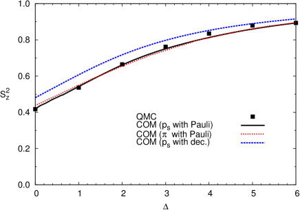
Figure 2: (Color online) The squared local magnetic moment per site of $d$ electrons $S_{z}^{2}$ as a function of $\Delta$ for $U=6$, $n_{T}=3$ and $T=1/3$ ($t_{pp}=0$). The solid black line refers to the COM results obtained using the field $p_{s}$ in the operatorial basis and the algebra constraints coming from the Pauli principle in the self-consistent scheme, the dashed blue to the field $p_{s}$ and the decoupling, and the dotted red line to $\hat{\pi}$ and the Pauli principle. The black squares are qMC data from Dopf et al. (1990).

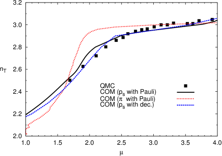
Figure 3: (Color online) The total filling $n_{T}$ versus the chemical potential $\mu$ is reported for $U=6$, $\Delta=4$ and $T=1/3$ ($t_{pp}=0$). The solid black line refers to the COM results obtained using the field $p_{s}$ in the operatorial basis and the algebra constraints coming from the Pauli principle in the self-consistent scheme, the dashed blue to the field $p_{s}$ and the decoupling, and the dotted red line to $\hat{\pi}$ and the Pauli principle. The black squares are qMC data from Dopf et al. (1990).

IV.1 Comparison with numerical simulations

In this Section, we compare the results obtained within the COM framework with those available in the literature, coming from a numerical analysis performed by means of qMC method Dopf et al. (1990). As it has been already shown in Fiorentino et al. (2001), the agreement within the Emery model between the numerical and the COM results is excellent. In particular, the computational schemes related to the first choice of the basis (both the one involving the algebra constraints coming from the Pauli principle and the one exploiting the decoupling procedure) give an excellent agreement with qMC for several quantities ($S_{z}^{2}$, $\mu$, band occupations, etc). In the present paper, we want to test the second possible choice of the basis and its self-consistent scheme in order to asses the overall stability and efficiency of the COM framework for the Emery model. Given the very comprehensive comparative analysis performed in Fiorentino et al. (2001) between COM and available numerical results, we have here limited our comparative analysis to just two quite relevant cases. Anyway, it is worth noticing that the second choice of the basis returns results in excellent agreement with the numerical ones also for all other quantities analyzed in Fiorentino et al. (2001) using the first choice. Hereafter, all energies are given in units of $t_{pd}$ and measured with respect to the atomic level $\varepsilon_{p}=0$.

In Fig. 2, we report the squared local magnetic moment per site of $d$ electrons $S_{z}^{2}=\frac{1}{4}\left\langle\left(n_{\uparrow}^{d}(\mathbf{i})-n_{\downarrow}^{d}(\mathbf{i})\right)^{2}\right\rangle$ as a function of $\Delta$ for $U=6$, $n_{T}=3$ and $T=1/3$. In the paramagnetic case, $S_{z}^{2}$ can be expressed Fiorentino et al. (2001) through the double occupancy of $d$ electrons $D$ and the number operator for $d$ electrons $n_{d}$ as $S_{z}^{2}=n_{d}-2D$. $D$ can be, in turn, computed directly in terms of correlation functions involving elements of the chosen operatorial basis: $D=\frac{n^{d}}{2}-C_{33}$. It is evident that the agreement with qMC result is very good in all three cases, especially when one uses the algebra constraints embedding the Pauli principle. $S_{z}^{2}$ takes the smallest value when $\Delta$ approaches zero as, in this case, the $p$ level and the $d$ upper Hubbard subband coincide and the strong hybridization enhances the $d$ electron double occupancy. On the other hand, when $\Delta$ becomes larger than $U$ the system moves from a charge-transfer to a Mott-Hubbard insulator and $S_{z}^{2}$ becomes independent from $\Delta$.

In Fig. 3, the dependence of the total filling $n_{T}$ on the chemical potential $\mu$ is reported for $U=6$, $\Delta=1$ and $T=1/3$. In this case too, we find a good agreement between COM results and qMC ones: the better agreement is reached for the solution having the field $p_{s}$ in the operatorial basis and the decoupling in the self-consistent scheme. The behavior of the chemical potential close to half filling ($n_{T}=3$) – the curve if not completely flat is just very little tilted because of the quite high value of the temperature – shows clear evidences of the opening of a gap.

It is worth noticing that the COM formulation is fully self-consistent and no adjustable parameter is used. Different choices of the operatorial basis, and of the related self-consistent scheme, return qualitatively similar results and definitely good and absolutely comparable benchmarks with respect to the numerical results. In the following, we will mainly use the solution having the field $p_{s}$ in the operatorial basis and the decoupling in the self-consistent scheme since this is the option that provides the higher numerical stability.

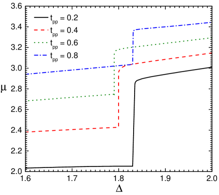
Figure 4: (Color online) The chemical potential $\mu$ as a function of $\Delta$ for $U=6$, $T=0.01$, $n_{T}=3$ and various values of $t_{pp}$.

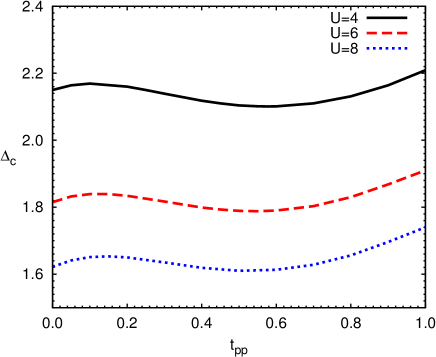
Figure 5: (Color online) The critical value of $\Delta$, $\Delta_{c}$, as a function of $t_{pp}$ for $T=0.01$, $n_{T}=3$ and various values of $U$.

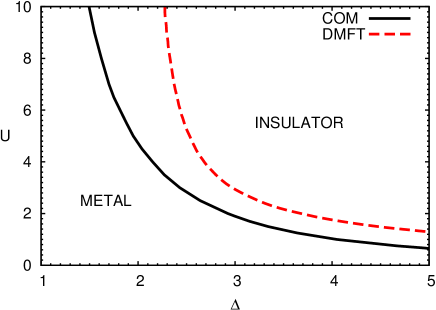
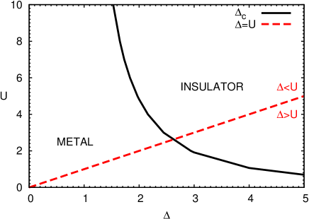
Figure 6: (Color online) Left panel: MIT phase diagram of the Emery model for $T=0.01$, $n_{T}=3$ and $t_{pp}=0$: black solid line refers to COM results, dashed red line to DMFT ones Ōno et al. (2001). Right panel: MIT phase diagram of the Emery model for phase diagram for $T=0.01$, $n_{T}=3$ and $t_{pp}=0.2$ within COM (solid black line). The dashed red line is a guide to the eye and separates the charge-transfer and Mott-Hubbard regimes in the insulator region.

IV.2 Metal-Insulator Transition

The metal-insulator transition (MIT) has been observed in many transition-metal oxides with more or less exotic physical properties Mott (1990); Imada et al. (1998). MIT has been largely studied in the single-band Hubbard model Imada et al. (1998); Mancini (2000), whose peculiar behavior gives the name to one of the fundamental types of MIT (paramagnetic, homogenous, due to the strong local Coulomb repulsion). According to Zaanen et al. (1985), the Emery model is instead the stage for two different types of MIT corresponding to two different regimes mainly ruled by the relationship between $U$ and $\Delta$. In particular, if $U>\Delta$ ($\varepsilon_{p}>\varepsilon_{d}$), the system is said to be in the charge-transfer (CT) insulating regime and the energy gap is roughly given by $\Delta$. On the contrary, if $U<\Delta$ ($\varepsilon_{p}<\varepsilon_{d}$), the system is said to be in the Mott-Hubbard (MH) regime and the energy gap is roughly given by $U$. This is easily understandable in terms of the relative positions of the $p$ level ($\varepsilon_{p}$) and of the two $d$ type Hubbard sub-bands ($\varepsilon_{d}$ and $\varepsilon_{d}+U$). Given that $\varepsilon_{p},\varepsilon_{d}<\varepsilon_{d}+U$, i.e. given that the first unoccupied level always belongs to the upper sub-band $\varepsilon_{d}+U$, we can have that the last occupied level either belongs to $\varepsilon_{p}$ in a CT or to $\varepsilon_{d}$ in a MH. The size of the gap follows immediately.

In the present paper, the study of the MIT in the Emery model has a two-fold aim: on one hand, we are interested in the mere occurrence of the MIT in the model and in its characterization through the analysis of its properties; on the other hand, our findings will shed some more light onto the puzzling physics of cuprates. In particular, we will discuss the relationship between the ab-initio determination of the model parameters proper for cuprates and the values of the model parameters required by many-body treatments in order to reproduce the experimental results.

We start from the first objective and explore the MIT in the whole range of values of the on-site potential $U$, the charge-transfer gap $\Delta$, and hopping integral between the oxygen orbitals $t_{pp}$. The MIT manifests itself in various properties of the system. Some of these properties are particularly suitable for the precise determination of the MIT onset within the COM framework. These fully equivalent MIT criteria are (at $T\approx 0$ and $n_{T}=3$): i) the presence of a jump in the chemical potential as a function of $\Delta$ or $U$ and ii) the opening of a gap in the density of states (DOS) at the Fermi level on varying $\Delta$ or $U$. The results presented in this subsection have been obtained by using the first criterion, namely the jump in $\mu(\Delta)$. It follows from ab-initio calculations for single-layer cuprates Kent et al. (2008) that typical values of the ratio $t_{pp}/t_{pd}$ range between $0.16$ and $0.7$. As shown in Fig. 4, by varying $t_{pp}$ within this range, we obtain a series of jumps in the dependence $\mu(\Delta)$. At the MIT, the chemical potential jumps between the upper Hubbard sub-band of copper main character and the band of mixed character that will be later related to the ZRS. We can immediately see that the critical value of $\Delta$, $\Delta_{c}$, has no monotonous behavior as a function of $t_{pp}$. The effective dependence of $\Delta_{c}$ on $t_{pp}$ is shown in Fig. 5. It is now evident that $t_{pp}$ does not significantly influence the overall value of $\Delta_{c}$, once $U$ is fixed. As $t_{pp}$ increases, $\Delta_{c}$ only slowly varies around a mean value up to $t_{pp}\approx 0.8$, while for greater values of $t_{pp}$ it starts growing quite rapidly. Interestingly, as $U$ increases, the whole curve $\Delta_{c}(t_{pp})$ rigidly moves downwards, almost without changing its overall shape. With respect to the MIT, it is evidently $U/\Delta$ the main player among the model parameters, but it is also clear that $t_{pp}$ can play a significative role in order to fine tune the results between different materials within the same class.

In the left panel of Fig. 6, we plot the phase diagram of the Emery model at $T=0.01$, $n_{T}=3$ and $t_{pp}=0$. The black solid and red dashed lines mark the phase boundary separating the metallic and the insulating regions given by COM and DMFT Ōno et al. (2001), respectively. The two critical curves are in quite good qualitative agreement with each other. The DMFT curve lays above the COM one, underestimating, with respect to the latter, the insulating phase, i.e. requiring rather higher values of $\Delta$ and $U$ to realize the MIT (see more below). In the right panel of Fig. 6, we plot $\Delta_{c}$ as a function of $U$ for $T=0.01$, $n_{T}=3$ and $t_{pp}=0.2$ (black solid line). The Mott-Hubbard regime is separated from the charge-transfer one by the red dashed line. One immediately notice that $\Delta_{c}$ increases quite rapidly on decreasing $U$. In the Mott-Hubbard regime, the metallic phase occurs only for small values of $U$ ($U<2.6$). On the other hand, in the charge-transfer regime, no metallic phase is observed for $\Delta\gtrsim 2.6$. For small values of $\Delta$, the system is metallic even in the limit $U\to\infty$, as already pointed out in Zaanen et al. (1985); Ōno et al. (2001). For $U>4$, the transition is always of charge-transfer type with $\Delta\lesssim 2.6$. On the other hand, it is known that several many-body treatments fail to reproduce the insulating behavior at half filling Kent et al. (2008) unless $\Delta$ exceeds $3\>eV$. Assuming a reasonable value of $t_{pd}\approx 1e\>V$ Kent et al. (2008), in our analysis we naturally obtain the charge-transfer insulator for a wider range of $\Delta$ and $U$ without any adjustment, thus being more consistent with the ab-initio predictions for $\Delta_{c}$ in cuprates that hardly exceed $3\>eV$ Kent et al. (2008) than other many-body treatments that seems to underestimate the insulating phase.

IV.3 Single-particle properties and ZRS

In this section, we analyze the single-particle properties of the Emery model (the energy bands, their spectral weights, orbital characters, and effective tight-binding parameters, and the density of states) as well as the occupations per orbital and band. The purpose of this study is (i) to fully characterize the low-energy excitations in momentum, band and orbital, (ii) to qualitatively and quantitatively analyze the hybridization between copper and oxygen orbitals and (iii) to assess the validity of the ZR scenario and establish its limitations.

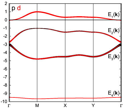
Figure 7: (Color online) Electronic dispersion in momentum space along the path $\mathrm{\Gamma=(0,0)}\to\mathrm{M}=(\pi,\pi)\to\mathrm{X=(\pi,0)}\to\mathrm{Y}=(0,\pi)\to\mathrm{\Gamma}$ for $n_{T}=3$, $\Delta=2$, $t_{pp}=0.2$, $T=0.01$, and $U=6$. The width of the bands is proportional to their spectral weights as functions of the momentum per orbital character: the $p$- and $d$- orbital characters are depicted with black and red colors, respectively.

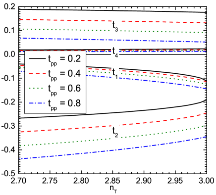
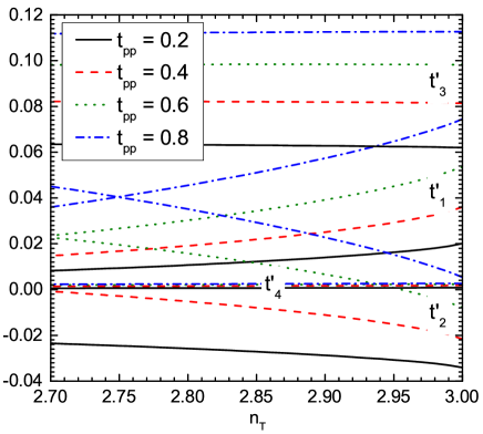
Figure 8: (Color online) Total filling ($n_{T}$) dependence of the effective nearest-neighbor ($t_{n}$, top panel) and next-nearest-neighbor ($t_{n}^{\prime}$, bottom panel) hopping integrals of the four bands $E_{n}(\mathbf{k})$ at $\Delta=\Delta_{c}$, $U=6$, $T=0.01$ and various values of $t_{pp}$.

IV.3.1 Bands

The adopted four-pole approximation obviously returns a four-band structure ($E_{n}(\mathbf{k})$ with $n=1,\ldots,4$) for the electronic dispersion of the Emery model, as it can be clearly seen in Fig. 7, where the latter is reported as a function of the momentum along the path $\mathrm{\Gamma=(0,0)}\to\mathrm{M}=(\pi,\pi)\to\mathrm{X=(\pi,0)}\to\mathrm{Y}=(0,\pi)\to\mathrm{\Gamma}$ for $n_{T}=3$, $\Delta=2$, $t_{pp}=0.2$, $T=0.01$, and $U=6$. The fictitious width of the four bands is proportional to their spectral weights as functions of the momentum per orbital character: $\sigma_{p}^{(n)}(\textbf{k})=\sigma_{11}^{(n)}(\textbf{k})$ and $\sigma_{d}^{(n)}(\textbf{k})=\sum_{a,b=2}^{3}\sigma_{ab}^{(n)}(\textbf{k})$. The $p$- and $d$- orbital characters are depicted with black and red colors, respectively. Given the center-of-mass positions of the four bands, their dependences on momentum and their dominant orbital characters: $E_{1}$ and $E_{4}$ can be safely assigned to the two Hubbard sub-bands of $d$ electrons (upper and lower, respectively), $E_{3}$ to the bare $p$ electron level and $E_{2}$ to the band arising from the ZR conjecture, i.e. to the dispersion related to the one-particle removal process out of the ZRS. Accordingly, four is exactly the minimal number of basic fields necessary to describe these very elementary excitations, whose presence in the system is quite well established Zaanen et al. (1985). Let us discuss now, one by one, the relevant and peculiar features of these four bands.

As regards the momentum dependence, a very simple way to analyze it just requires to Fourier transform back to real space each of the four bands separately. It is definitely worth pointing out that this very systematic analysis also permits to investigate in detail the possibility to reduce the system to an effective two-band one. This simple, but efficient, procedure returns the effective tight-binding parameters per band as modified, with respect to the bare ones present in the Hamiltonian, by the interactions, the hybridizations and the related high-order real and virtual processes. As shown in Fig. 8, $E_{1}$ and $E_{2}$ have sizable negative nearest-neighbor effective hopping integrals ($t_{1}$ and $t_{2}$, respectively), in agreement with the presence of a minimum at $\Gamma$ and of a maximum at $M$ (see Fig. 7). The situation is completely reversed for $E_{3}$ and $E_{4}$. All bands, except for $E_{4}$ that is almost flat, have non-negligible next-nearest-neighbor (along main diagonals) effective hopping integrals ($t_{i}^{\prime}$), in agreement with the presence of a warp along the $X\to Y$ direction (see Fig. 7). The apparent dominance (see Fig. 7) of the $\alpha(\mathbf{k})$ component in the dispersion (among the 2D cubic harmonics) is reflected in the prevalence of $t_{n}$ on longer-distance hopping integrals. Given the hopping and the hybridization terms present in the Hamiltonian (4), the $\alpha(\mathbf{k})$ component of the dispersion is dynamically generated by the second-order process describing the indirect hopping between nearest-neighbor copper sites involving an intermediate oxygen site (i.e. $t_{n}\propto t_{pd}^{2}$ and $\gamma^{2}(\textbf{k})=1-\alpha(\mathbf{k})$). Similarly, it is the Hamiltonian term responsible for the direct hopping between nearest-neighbor oxygens to induce a finite value of the next-nearest-neighbor (along main diagonals) effective hopping integrals ($t_{i}^{\prime}$). It also induces the related $\beta(\mathbf{k})$ component of the dispersion, which drives the warp along the $X\to Y$ direction. These two occurrences are based on the third-order process describing the indirect hopping between next-nearest-neighbor (along main diagonals) copper sites involving two intermediate nearest-neighbor oxygen sites (i.e. $t^{\prime}_{n}\propto t_{pd}t_{pp}t_{pd}$ and $\lambda(\textbf{k})\gamma^{2}(\textbf{k})=1-2\alpha(\textbf{k})+\beta(\textbf{k})$). Accordingly, on top of the interactions, which play the main role in this, also $t_{pd}$ and $t_{pp}$ enter into the redefinition of the center-of-mass positions of the four bands. Moreover, the value of $t_{pp}$ affects the bandwidth of the four bands as it contributes to determine the value of $t_{n}$. Given these occurrences, it is now clear why $t_{pp}$ is usually considered the major discriminant among the different cuprate families or even specific materials. $E_{2}(\mathbf{k})$ features a finite next-nearest-neighbor effective hopping integral along main axes too (not shown).

The values of all effective hopping integrals are almost completely independent of $\Delta$ and $U$ (not shown); this occurrence opens up the possibility to use the two bands closer to the Fermi level, and in particular their effective hopping integrals (their tight-binding reduction), as constitutive elements of an effective two-band model as suggested by the ZR conjecture. On the other hand, the dependence of the same effective hopping integrals on the total filling $n_{T}$ is not negligible (see Fig. 8). This latter occurrence does not contradict the ZR conjecture as the hopping integrals of the effective two-band model can assume effective values on varying any external parameter (filling, temperature or any applied field). The center-of-mass positions of the four bands, as functions of $U$ for fixed $\Delta$, do not change (not shown) except for the lower Hubbard one ($E_{4}$). Such a behavior was foreseeable as $\Delta$ was kept constant, but only as regards the relative positions: the constancy of the chemical potential pins the absolute positions of the levels too. It is worth noting that the electronic dispersion close to the Fermi level has an overall shape in very good agreement with what found by the ab-initio calculations.

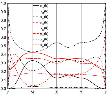
Figure 9: (Color online) Spectral weights per orbital character as functions of the momentum along the path $\mathrm{\Gamma}\to\mathrm{M}\to\mathrm{X}\to\mathrm{Y}\to\mathrm{\Gamma}$ for $n_{T}=3$, $\Delta=2$, $t_{pp}=0.2$, $T=0.01$, $U=6$. The $p$- and $d$- orbital characters are depicted with black and red colors, respectively.

Obviously, each of the four bands has mixed $p$- and $d$- character as it can be clearly seen in Fig. 9. The relative weight of the two species ($p$- and $d$-) is quite strongly momentum dependent and varies very much from band to band at fixed momentum. $E_{4}$ is mostly $d$-like, while $E_{1}$, $E_{2}$ and $E_{3}$ have fully mixed character with a slight predominance of the $d$ component in $E_{1}$ and of the $p$ component in $E_{2}$ and $E_{3}$. $E_{1}$ shows a net prevalence of the $d$ component at the $\Gamma\;(0,0)$ point, which hosts the minimum of the band, in perfect agreement with the well established fact that the first electronic addition should have definite $d$ character. Similarly, the ratio between the $p$- and $d$- character ($3:2$), at the maximum of the $E_{2}$ band (the $M(\pi,\pi)$ point), agrees very well with the evidences for a mainly $p$ character for the first electronic removal, as also required by the ZRS conjecture. This latter also requires an almost identical slope in momentum space of the two components at the $M$ point, as it is apparent in Fig. 9. In $E_{2}$, the two components exchange their relative relevance going from the $\Gamma$ point ($d$-predominance) towards the $M$ point ($p$-predominance). In $E_{3}$, the two components have the tendency to occupy similarly and quite uniformly the momentum space except at the $\Gamma$ point, where $d$-electrons are simply absent. $E_{4}$, according to its extreme flatness, has a uniform occupation in momentum space. In conclusion, the ZR scenario is fully supported by our findings as they show that doping the system out of half filling ($n_{T}=3$) generates holes in the $E_{2}$ band at $(\pi,\pi)$ with a dominant $p$-character and particles in the $E_{1}$ band at $(0,0)$ with definite $d$-character.

IV.3.2 Density of states

The densities of states for $p$- and $d$- orbital characters can be calculated according to the following formulas

$$\begin{split}N_{p}(\omega)&=\frac{a^{2}}{(2\pi)^{2}}\int_{\Omega_{B}}d^{2}\textbf{k}\sum_{n=1}^{4}\sigma_{11}^{(n)}(\textbf{k})\delta(\omega-E_{n}(\textbf{k}))\\ N_{d}(\omega)&=\frac{a^{2}}{(2\pi)^{2}}\int_{\Omega_{B}}d^{2}\textbf{k}\sum_{n=1}^{4}\left[\sigma_{22}^{(n)}(\textbf{k})+2\sigma_{23}^{(n)}(\textbf{k})\right.\\ &+\left.\sigma_{33}^{(n)}(\textbf{k})\right]\delta(\omega-E_{n}(\textbf{k})).\end{split}$$ (40)

These densities of states, presented in Fig. 10, clearly show the positions of the van Hove singularities together with the marked enhancements (in particular, in $E_{1}$ and $E_{2}$) coming from the warp in the dispersion along the $X\to Y$ direction due to the finite value of $t_{pp}$. The already discussed mixed $p$- and $d$- character of the four bands is evident once more and the strong energy dependence of the relative weight of the two species ($p$- and $d$-) is clearly visible. The very high degree of hybridization between the two species, in particular in the energy and momentum regions close to the Fermi surface, is another fundamental brick in the construction of an effective theory with a reduced number of degrees of freedom.

Figure 10: (Color online) Densities of states per orbital character for $n_{T}=3$, $\Delta=2$, $t_{pp}=0.2$, $T=0.01$ and $U=6$. The $p$- and $d$- orbital characters are depicted with (solid) black and (dashed) red colors, respectively.

IV.3.3 Band and orbital occupations

It is very interesting to analyze the distribution of the electrons among the four bands as well as between the $p$- and $d$- orbitals. The corresponding occupation numbers per band ($i=1,\ldots,4$) $n_{i}=n_{ip}+n_{id}$ and per orbital ($p$ or $d$)

$$n_{p}=\sum_{i=1}^{4}n_{ip}\qquad\qquad n_{d}=\sum_{i=1}^{4}n_{id}$$

can be obtained properly summing up the following basic quantities

$$\begin{split}n_{ip}&=\frac{a^{2}}{(2\pi)^{2}}\int_{\Omega_{B}}d^{2}\textbf{k}\left(1-T_{i}(\textbf{k})\right)\sigma_{11}^{(i)}(\textbf{k})\\ n_{id}&=\frac{a^{2}}{(2\pi)^{2}}\int_{\Omega_{B}}d^{2}\textbf{k}\left(1-T_{i}(\textbf{k})\right)\times\\ &\times\left(\sigma_{22}^{(i)}(\textbf{k})+\sigma_{33}^{(i)}(\textbf{k})+2\sigma_{23}^{(i)}(\textbf{k})\right)\end{split}$$

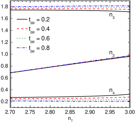
Figure 11: (Color online) Occupation numbers per band $n_{2}$, $n_{3}$ and $n_{4}$ ($n_{1}=0$) as functions of the total density $n_{T}$ for different values of $t_{pp}$ at $\Delta=\Delta_{c}(t_{pp})$ for $T=0.01$ and $U=6$.

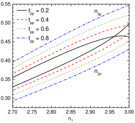
Figure 12: (Color online) Occupation numbers of the $E_{2}$ band per orbital character $n_{2p}$ and $n_{2d}$ as functions of the total density $n_{T}$ for different values of $t_{pp}$ at $\Delta=\Delta_{c}(t_{pp})$ for $T=0.01$ and $U=6$.

It is worth noting that the band structure of the Emery model determines and is, in turn, determined by the occupations per band of the $p$- and $d$- electrons. The analysis of such occupations per band reveals that they are independent of $U$ (not shown), favoring the reduction to an effective single-band model, although this is due to a compensation of the $p$- and $d$- components within each band (not shown). In particular, the $p$- and $d$- fillings in the band $E_{2}$ change quite much upon varying $U$, but conserving their sum, and so the overall filling of the band, practically constant. The reason behind this redistribution is quite easy to understand: the on-site Coulomb repulsion $U$ is the main control of the overall amount of double occupancy of the $d$ component and, consequently, is also responsible for the fine tuning of the ratio between the $p$- and $d$- components within the ZRS.

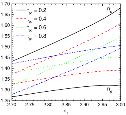
Figure 13: (Color online) Occupation numbers per orbital character $n_{p}$ and $n_{d}$ as functions of the total density $n_{T}$ for different values of $t_{pp}$ at $\Delta=\Delta_{c}(t_{pp})$ for $T=0.01$ and $U=6$.

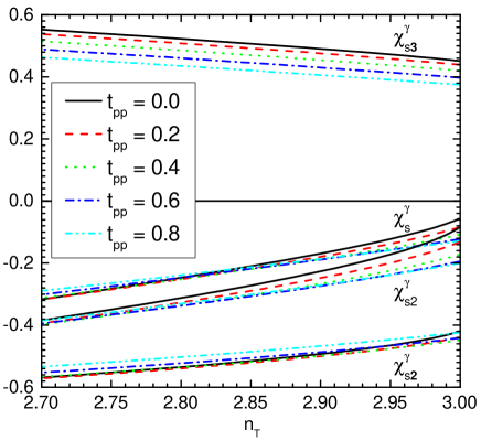
Figure 14: (Color online) Plaquette $p$-$d$ spin correlation function and its per-band decomposition as functions of the total density $n_{T}$ for different values of $t_{pp}$ at $\Delta=\Delta_{c}(t_{pp})$ for $T=0.01$ and $U=6$.

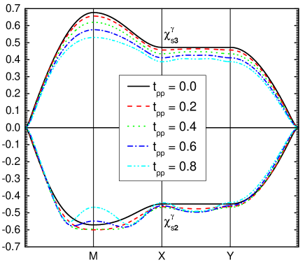
Figure 15: (Color online) Plaquette $p$-$d$ spin correlation function decomposed per band as function of the momentum along the path $\mathrm{\Gamma}\to\mathrm{M}\to\mathrm{X}\to\mathrm{Y}\to\mathrm{\Gamma}$ for $n_{T}=3^{-}$, different values of $t_{pp}$, $\Delta=\Delta_{c}(t_{pp})$, $T=0.01$ and $U=6$.

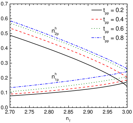
Figure 16: (Color online) Hole occupation numbers of the $E_{1}$ and the $E_{2}$ band per $p$ orbital character $n_{2p}$ and $n_{2d}$ as functions of the total density $n_{T}$ for different values of $t_{pp}$ at $\Delta=\Delta_{c}(t_{pp})$ for $T=0.01$ and $U=6$.

In Fig. 11, it is clearly shown that upon doping, the holes go primarily into the $E_{2}$ band, while the occupation of the other bands remains almost unchanged: the practical constancy of the occupations of the $E_{3}$ and $E_{4}$ bands conveys the doping only to the $E_{2}$ band, once more justifying a reduction to an effective single-band Hubbard model. It is really remarkable that at the MIT, marked by the vanishing of the occupation $n_{1}$ of the upper Hubbard sub-band $E_{1}$, the occupation $n_{2}$ of the band $E_{2}$ crosses one (see again Fig. 11). This occurrence opens up the possibility to mime such a MIT of charge-transfer type through a MIT of Mott-Hubbard type according to the ZR construction. This latter construction also requires that, upon doping, the copper and oxygen occupations of the band $E_{2}$ decrease with the same slope: as reported in Fig. 12, except for the doping region really very close to the MIT or for too high values of $t_{pp}$, this is the case. Across all four bands, the great majority of the doping goes in the oxygen channel (see Fig. 13) as expected Zhang and Rice (1988).

In order to characterize further the two bands closer to the chemical potential and with mainly $p$ character ($E_{2}$ and $E_{3}$), we have analyzed the spin-spin correlation function between the $p$-bonding hole projected on the plaquette and the central $d$ hole: $\chi_{s}^{\gamma}=\frac{1}{3}\left\langle\hat{p}^{\dagger\gamma}\sigma_{k}\hat{p}^{\gamma}\hat{n}_{k}^{d}\right\rangle=\frac{2}{3}\left(C_{14}^{\gamma}+\frac{3c}{I_{22}}C_{12}^{\gamma}+\frac{3b}{I_{33}}C_{13}^{\gamma}\right)$. The hatted operators stand for their hole counterparts given by a particle-hole transformation ($\psi_{\sigma}(i)\to(-1)^{|i|}\hat{\psi}_{\sigma}^{\dagger}(i)$). In Fig. 14, we report $\chi_{s}^{\gamma}$ as a function of the total density $n_{T}$ and its components per band $\chi_{sn}^{\gamma}$ in the hole representation. We also report its components per band $\chi_{s\mathbf{n}}^{\gamma}$ computed without taking into account the actual occupation of the related bands (i.e. without weighting the inner momentum components by the appropriate Fermi function). In this way, we can analyze the features of the contributions not activated yet by the actual hole doping level. $\chi_{s}^{\gamma}$ is negative in the whole range of doping explored and becomes more and more negative on increasing the doping: the holes doped in the system not only have mainly $p$ character and $E_{2}$ location, but they also form plaquette states of singlet type with the $d$ holes - as predicted by ZR conjecture. The actual contribution of the band $E_{2}$ ($\chi_{s2}^{\gamma}$) is prevalent, as can be clearly seen in Fig. 14. Upon comparing the non-Fermi-weighted contributions of the bands $E_{2}$ and $E_{3}$ ($\chi_{s\mathbf{2}}^{\gamma}$ and $\chi_{s\mathbf{3}}^{\gamma}$, respectively), we can clearly establish the singlet nature of the excitations populating the band $E_{2}$ and the triplet nature of the excitations populating the band $E_{3}$. As a matter of fact, the bonding component of the $p$ orbital further splits in a singlet and a triplet components (bands $E_{2}$ and $E_{3}$, respectively) according to the spin coupling to the $d$ orbital on the plaquette. This is also confirmed by the further decomposition in momentum space of $\chi_{s\mathbf{2}}^{\gamma}$ and $\chi_{s\mathbf{3}}^{\gamma}$ reported in Fig. 15. It is worth noting the negative effects of increasing $t_{pp}$ on the net separation between singlets and triplets (see Figs. 14 and 15).

Finally, comparing our results with XAS oxygen K-edge experiments Peets et al. (2009), we confirm the impossibility to observe a saturation of the low-energy spectral weight in the overdoped region in a three-band model Wang et al. (2010) without taking the oxygen intrasite Coulomb repulsion into account (see behavior of $n_{2p}^{h}$, the hole occupation of $p$ character in band $E_{2}$, in Fig. 16). On the other hand, the systematic reduction of the measured oxygen K-edge intensity assigned to the upper Hubbard band Peets et al. (2009) is well described in our formulation (see behavior of $n_{1p}^{h}$, the hole occupation of $p$ character in band $E_{1}$, in Fig. 16) as it can be understood in terms of oxygen-hole spectral-weight transfer between the upper Hubbard band ($E_{1}$) and the ZRS band ($E_{2}$) driven by the gain in energy at the basis of the mechanism leading to the ZRS formation.

All these findings highlight once more the strict connection between the two components (i.e. the extremely high degree of hybridization) and confirm the soundness of the reduction process to an effective single-band model in the underdoped regime.

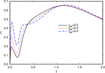
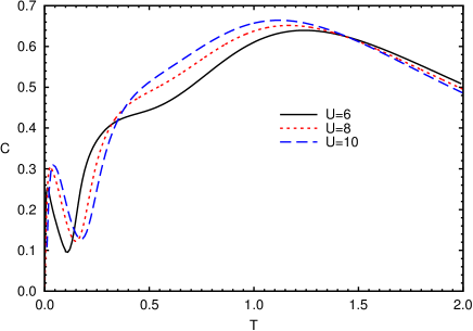
Figure 17: (Color online) The specific heat $C$ as a function of the temperature $T$ for $n_{T}=3$, $\Delta=2$ and: (top panel) $U=8$ and various values of $t_{pp}$; (bottom panel) $t_{pp}=0.2$ and various values of $U$.

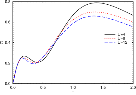
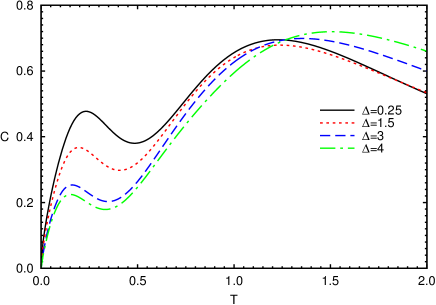
Figure 18: (Color online) The specific heat $C$ as a function of the temperature $T$ for $n_{T}=2.7$, $t_{pp}=0.2$ and: (top panel) $\Delta=3$ and various values of $U$; (bottom panel) $U=8$ and various values of $\Delta$.

IV.4 Thermodynamic properties

In this section, we report about the thermodynamic properties at finite temperature of the Emery model. In particular, we focus our attention on two thermodynamic quantities, namely the specific heat $C$ and the entropy $S$, and on their temperature dependence on varying the model parameters. Assuming a different perspective with respect to that acquired by studying the single-particle properties in the previous sections, this analysis will allow to collect further pieces of information on the most relevant energy scales of the system.

IV.4.1 Specific heat

The specific heat $C$ is defined as $C=dE/dT$, where the internal energy $E$ can be computed as the thermal average of the Hamiltonian (1) as

$$E=\varepsilon_{d}n_{d}+\varepsilon_{p}n_{p}+UD-8t_{pd}(C_{12}^{\gamma}+C_{13}^{\gamma})-4t_{pp}C_{11}^{\lambda}.$$ (41)

At half filling, $n_{T}=3$, the specific heat presents three peaks (see Figs. 17). We wish to remind that a peak in the specific heat at a certain temperature is usually related to the presence of an enhancement in the density of states at an energy, with respect to the chemical potential, about twice larger. The presence of a peak at the lower temperatures is due to the pinning of the chemical potential in the proximity either of the very top of the band $E_{2}$ (at $M(\pi,\pi)$) or of the bottom of the band $E_{1}$ (at $\Gamma(0,0)$) and to the flatness of the bands at these points that induces very intense peaks in the density of states (not shown). Such an occurrence enormously enhances the number of states available at small temperatures and determines the presence of the corresponding peak in the specific heat. Consequently, the evident dependence on $t_{pp}$ of both the position in temperature and the height of this peak (see Fig. 17 (top panel)) is related to the obvious effects $t_{pp}$ has on the relative position in energy, with respect to the antidiagonal $X\to Y$, and flatness of both the top of the band $E_{2}$ and the bottom of the band $E_{1}$. A similar discussion holds for the dependence on $U$ as shown in Fig. 17 (bottom panel). At any rate, this peak is not very fundamental as it can be considered an accident and much probably would not have any experimental relevance. The second peak, centered at about $T\approx 0.25$ and more evident at large $t_{pp}$ and small $U$, is connected to the enhancement in the density of states driven by the van Hove singularity closest to the position of the chemical potential. Given the tight-binding effective reduction and the related explanation reported in the previous section, in both cases (whether the chemical potential lies in $E_{1}$ or $E_{2}$) this distance in energy is about $0.5$ and varies with $t_{pp}$ and $U$ as shown by the actual position of the peak (see Figs. 17). Finally, the third peak, the one centered at about $T\approx 1$, is due to the van Hove singularity of the other band with respect to the one where the chemical potential lies. In this case, the distance in energy is mainly due to $\Delta$ and varies very little with $t_{pp}$ while is much more sensitive to $U$, as clearly expected.

Away from half filling, at $n_{T}=2.7$, the specific heat presents only two peaks (see Figs. 18). Taking into account that for this filling the chemical potential lies inside of the band $E_{2}$ and close to its van Hove singularity, the positions in temperature of these two peaks can be ascribed to the relative positions of the top of the band $E_{2}$ and to the position of the van Hove singularity in the band $E_{1}$. It is quite interesting to verify that $U$ does not affect the position and the height of the first peak (see Fig. 18 (top panel)), as one would expect since the overall shape and population of the band $E_{2}$ is not very affected by $U$, while $U$ has a quite visible effect on the height of the second peak, but not on its position. The average distance between the two bands, that is, between the two centers of mass, which can be mainly identified with the positions of the van Hove singularities, is determined by $\Delta$ and not by $U$ in the charge-transfer regime, where the model lies for these values of the model parameters. On the other hand, $U$ definitely reduces the number of available states in the upper Hubbard sub-band $E_{1}$ and consequently reduces the height of the second peak. In the metallic regime (for $\Delta<\Delta_{c}$), $\Delta$ can, instead, enhance quite much the height of the first peak, although it cannot change its position, as it can influence the flatness of the top of the band $E_{2}$ in order to accommodate more and more moving particles. On the other hand, $\Delta$ can change the position and, slightly, the height of the second peak only in the insulating regime (for $\Delta>\Delta_{c}$) as it can influence the distance of the band $E_{1}$ in order to determine the charge gap.

According to the above analysis, an experimental measurement of the specific heat can help determining the values of some of the model parameters for an effective model.

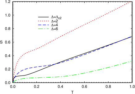
Figure 19: (Color online) The entropy $S$ as a function of the temperature $T$ for $n_{T}=3$, $t_{pp}=0.2$, $U=8$ and various values of $\Delta$.

IV.4.2 Entropy

The entropy has been computed through the following relation to the specific heat

$$S(T)=\int_{0}^{T}\frac{C(T^{\prime})}{T^{\prime}}\,dT^{\prime}.$$ (42)

In Fig. 19, we report its behavior as a function of the temperature at half filling, $n_{T}=3$, in the charge-transfer ($U>\Delta$) insulating ($\Delta\geq\Delta_{c}$) regime. The great enhancement at low temperatures is due to the first peak in the specific heat and, as this latter, can be considered accidental. Definitely more interesting is the subsequent inflection. It is more or less pronounced according to the height and capability to resolve the second peak and is one to one related to the presence of the gap between the two bands close to the chemical potential and so to the insulating nature of the system. Accordingly, an experimental measure of the entropy could give fundamental information about the size of the gap in the system.

V Conclusions

In the present manuscript, we have considered the Emery model within the COM method. With respect to what already done in Fiorentino et al. (2001), we have introduced a finite direct oxygen hopping $t_{pp}$ and focused on the single-particle properties in order to discuss the validity and range of applicability of the ZR construction and scenario. We first introduced the model and its reduction to the bonding component only of the oxygen orbital. Then, we checked two possible choices for the basic field and the related self-consistency equations. Both choices have been found to give results in very good agreement with the available numerical ones, being one of the two choices (the one used in the rest of the manuscript) more numerically stable and so suitable for systematic and massive use.

Within COM, we observe a metal-insulator transition at half filling ($n_{T}=3$) and our critical line agrees quite well with the one obtained within DMFT Ōno et al. (2001). Two regimes can be clearly distinguished: a Mott-Hubbard regime ($U<\Delta$) and a charge-transfer one ($U>\Delta$). The ab-initio deduced parameter values relevant for cuprates bring us into the charge-transfer regime without any adjustment, unlike many other analytical methods. We also studied the influence of the finite direct oxygen hopping on the MIT.

Analyzing the single-particle properties of the model, we validated the ZR scenario as we found the first hole excitations to be of mainly oxygen type at $(\pi,\pi)$ and the first electronic excitations to be of mainly copper type at $(0,0)$. Moreover, the reduction to an effective two-band model resulted definitely feasible as the doping goes all in one of the four bands, compensates correctly between oxygen and copper given the very high degree of hybridization found both in energy and momentum, and the tight-binding effective hoppings results independent on $U$ and $\Delta$. We also found that the overall shape of the bands close to the chemical potential is quite similar to that given by the available ab-initio calculations.

Finally, the analysis of the specific heat and of the entropy allowed to determine a strict connection between the features of these latter, in principle experimentally measurable, and the relevant model parameters.

Appendix A Details of calculations

A.1 Basis I

If we do consider the basis (5), the normalization matrix $I(\mathbf{k})$ has the expression

$$I(\mathbf{k})=\left({\begin{array}[]{cccc}1&0&0&0\\ 0&{I_{22}}&0&0\\ 0&0&{I_{33}}&0\\ 0&0&0&{I_{44}}\end{array}}\right)$$ (43)

where

$$\begin{split}I_{22}&=1-\frac{n_{d}}{2}\\ I_{33}&=\frac{n_{d}}{2}\\ I_{44}&(\mathbf{k})=3[n_{d}-2D-\chi{\kern 1.0pt}_{s}\alpha(\mathbf{k})]+4a_{s}-\frac{9c^{2}}{I_{22}}-\frac{9b^{2}}{I_{33}}\end{split}$$ (44)

with

$${\begin{array}[]{lll}b&=&\langle p^{\gamma}(i)\eta^{{\dagger}}(i)\rangle\\ c&=&\langle p^{\gamma}(i)\xi^{{\dagger}}(i)\rangle\\ n_{d}&=&\langle n^{d}(i)\rangle\end{array}}\quad\;{\begin{array}[]{lll}D&=&\langle n_{\uparrow}^{d}(i)n_{\downarrow}^{d}(i)\rangle\\ a_{s}&=&\langle p^{\gamma}(i)p^{\dagger\gamma}(i)\sigma_{k}n_{k}^{d}(i)\rangle\\ \chi_{s}&=&\langle n_{k}^{d}(i)n_{k}^{d^{\alpha}}(i)\rangle/3.\end{array}}$$ (45)

The matrix $m(\mathbf{k})$ has the expression

$$m(\mathbf{k})=\left({\begin{array}[]{cccc}{m_{11}}&{m_{12}}&{\phantom{-}m_{13}}&0\\ {m_{12}}&{m_{22}}&{\phantom{-}m_{23}}&{\phantom{-}m_{24}}\\ {m_{13}}&{m_{23}}&{\phantom{-}m_{33}}&{-m_{24}}\\ 0&{m_{24}}&{-m_{24}}&{\phantom{-}m_{44}}\end{array}}\right).$$ (46)

and its entries are given by

$$\begin{split}m_{11}&=(\varepsilon_{p}-\mu)+2t_{pp}\lambda(\mathbf{k})\\ m_{12}&=2t_{pd}I_{22}\gamma(\mathbf{k})\\ m_{13}&=2t_{pd}I_{33}\gamma(\mathbf{k})\\ m_{22}&=(\varepsilon_{d}-\mu)I_{22}+2t_{pd}(c-b)\\ m_{23}&=-2t_{pd}(c-b)\\ m_{24}&=2t_{pd}I_{\pi p_{s}}(\mathbf{k})\\ m_{33}&=(\varepsilon_{d}-\mu+U)I_{33}+2t_{pd}(c-b)\\ m_{44}&=(\varepsilon_{p}-\mu)I_{44}(\mathbf{k})+t_{p}I_{\pi p_{s}}(\mathbf{k})\\ &+2t_{pd}I_{\kappa_{s}p_{s}}(\mathbf{k})+2t_{pp}I_{\lambda_{s}p_{s}}(\mathbf{k})\end{split}$$ (47)

where

$$\begin{split}I_{\pi p_{s}}&=\frac{3}{2}[n_{d}-\chi_{s}\alpha(\mathbf{k})]+\frac{1}{2}\hat{a}_{s}\\ &+3(c-b)(bI_{33}^{-1}-cI_{22}^{-1})\\ I_{\kappa_{s}\xi}&=\frac{3}{2}[n_{d}+\hat{a}_{s}-\chi_{s}\alpha(\mathbf{k})]-\frac{3c}{2t_{pd}}(U-\Delta)\\ I_{\kappa_{s}\eta}&=-\frac{3}{2}[n_{d}+\hat{a}_{s}-\chi_{s}\alpha(\mathbf{k})]+\frac{3b}{2t_{pd}}\Delta\\ I_{\lambda_{s}p_{s}}&=4a_{s\lambda}+3cc_{\lambda}I_{22}^{-1}+3bb_{\lambda}I_{33}^{-1}\\ &+3(n^{d}-2D)-6\chi_{s}\alpha(\mathbf{k})+3\chi_{s\beta}\beta(\mathbf{k})\\ I_{\kappa_{s}p_{s}}&=6[-b-f+d_{s}\alpha(\mathbf{k})]-4b_{s}\\ &+\frac{9}{2}(bI_{33}^{-1}-cI_{22}^{-1})[n_{d}+\hat{a}_{s}-\chi_{s}\alpha(\mathbf{k})]\\ &+\frac{9}{2t_{pd}}[c^{2}I_{22}^{-1}(U-\Delta)-b^{2}I_{33}^{-1}\Delta]\end{split}$$ (48)

with

$$\begin{split}b_{s}&=\langle d^{\alpha}(i)p^{\dagger\gamma}(i)\sigma_{k}n_{k}^{d}(i)\rangle\\ c_{\lambda}&=\langle p^{\gamma\lambda}(i)\xi^{{\dagger}}(i)\rangle\\ b_{\lambda}&=\langle p^{\gamma\lambda}(i)\eta^{{\dagger}}(i)\rangle\\ f&=\langle p^{\gamma}(i)d^{{\dagger}}(i)p^{\gamma}(i)p^{\gamma^{{\dagger}}}(i)\rangle\\ d_{s}&=\frac{1}{3}\langle n_{k}^{d\alpha}(i)\sigma_{k}p^{\gamma}(i)d^{{\dagger}}(i)\rangle\\ \hat{a}_{s}&=-2D+\frac{4}{3}a_{s}\\ a_{s\lambda}&=\langle p^{\gamma\lambda}(i)p_{s}^{\dagger}\rangle\\ \chi_{s\beta}&=\frac{1}{3}\langle n_{k}^{d}(i)n_{k}^{d{\beta}}(i)\rangle.\end{split}$$ (49)

By making use of Eqs. (48), it can be shown that the matrix element $m_{44}$ can be exactly expressed as $m_{44}=m_{44}^{0}+\alpha(\textbf{k})m_{44}^{\alpha}+\beta(\textbf{k})m_{44}^{\beta}$ with $m_{44}^{0}$, $m_{44}^{\alpha}$ and $m_{44}^{\beta}$ defined as:

$$\begin{split}m_{44}^{(0)}&=(\varepsilon_{p}-\mu)I_{44}^{(0)}+9[c^{2}I_{22}^{-1}(U-\Delta)-b^{2}I_{33}^{-1}\Delta]\\ &-4t_{pd}(3b+3f+2b_{s})\\ &+6t_{pd}(bI_{33}^{-1}-cI_{22}^{-1})(3n_{d}+\hat{a}_{s})\\ &+18t_{pd}(c-b)(bI_{33}^{-1}-cI_{22}^{-1})^{2}\\ &+2t_{pp}[4a_{s\lambda}+3cc_{\lambda}I_{22}^{-1}+3bb_{\lambda}I_{33}^{-1}+3(n_{d}-2D)]\end{split}$$

$$\begin{split}m_{44}^{(\alpha)}&=(\varepsilon_{p}-\mu)I_{44}^{(1)}\\ &+6t_{pd}[2d_{s}-3(bI_{33}^{-1}-cI_{22}^{-1})\chi_{s}]-12t_{pp}\chi_{s}\\ m_{44}^{(\beta)}&=6t_{pp}\chi_{sb},\end{split}$$

where we have introduced the quantities $I_{44}^{(0)}$ and $I_{44}^{(1)}$, which read as follows

$$\begin{split}I_{44}^{(0)}&=3n_{d}+\hat{a}_{s}-9c^{2}I_{22}^{-1}-9b^{2}I_{33}^{-1}\\ I_{44}^{(1)}&=-3\chi_{s}.\end{split}$$ (50)

A.2 Basis II

If we do consider the basis (20), the normalization matrix $I(\mathbf{k})$ has the expression given in (43) but with $I_{44}(\mathbf{k})$ given by

$$I_{44}(\mathbf{k})=a-I_{33}^{2}-I_{22}^{-1}g^{2}-I_{33}^{-1}g^{2}+f_{s}+(I_{33}^{2}-p)\alpha(\mathbf{k})$$

where

$$\begin{split}g&=\langle p^{\gamma}(i)\xi^{{\dagger}}(i)\rangle-\langle p^{\gamma}(i)\eta^{{\dagger}}(i)\rangle\\ a&=1-\langle p^{\gamma}(i)p^{{\dagger}}(i)\rangle-2\langle\pi(i)p^{\gamma{\dagger}}(i)\rangle\\ f_{s}&=2\langle\sigma_{k}n_{k}^{d}(i)p^{\gamma}(i)p^{\gamma{\dagger}}(i)\rangle\\ p&=\frac{1}{4}\langle n_{\mu}^{d}(i)n_{\mu}^{d^{\alpha}}(i)\rangle-\langle d_{\uparrow}(i)d_{\downarrow}(i)[d_{\downarrow}^{{\dagger}}(i)d_{\uparrow}^{{\dagger}}(i)]^{\alpha}\rangle\end{split}$$

The matrix $m(\textbf{k})$ has the same expression given in (47) and (48) but with $m_{44}(\textbf{k})$ given by

$$m_{44}(\textbf{k})=m_{44}^{(0)}+m_{44}^{(\alpha)}\alpha(\textbf{k})+m_{44}^{(\beta)}\beta(\textbf{k})$$

where

$$m_{44}^{(\beta)}=\frac{1}{4}\langle n_{\mu}^{d}(i)n_{\mu}^{d{\beta}}(i)\rangle-\langle d_{\uparrow}(i)d_{\downarrow}(i)[d_{\downarrow}^{{\dagger}}(i)d_{\uparrow}^{{\dagger}}(i)]^{\beta}\rangle$$

The quantities $m_{44}^{(0)}$ and $m_{44}^{(\alpha)}$ are calculated by imposing the algebra constraints embedding the Pauli principle.

References

- Dagotto (1994) E. Dagotto, Rev. Mod. Phys. 66, 763 (1994).
- Damascelli et al. (2003) A. Damascelli, Z. Hussain, and Z.-X. Shen, Rev. Mod. Phys. 75, 473 (2003).
- Lee et al. (2006) P. A. Lee, N. Nagaosa, and X.-G. Wen, Rev. Mod. Phys. 78, 17 (2006).
- Armitage et al. (2010) N. P. Armitage, P. Fournier, and R. L. Greene, Rev. Mod. Phys. 82, 2421 (2010).
- Anderson (1987) P. W. Anderson, Science 235, 1196 (1987).
- Emery (1987) V. J. Emery, Phys. Rev. Lett. 58, 2794 (1987).
- Emery and Reiter (1988) V. J. Emery and G. Reiter, Phys. Rev. B 38, 4547 (1988).
- Varma (1987) C. M. Varma, Solid State Commun. 62, 681 (1987).
- Gaididei and Loktev (1988) Y. B. Gaididei and V. M. Loktev, Phys. Status Solidi 147, 307 (1988).
- Loktev (1996) V. Loktev, Fizika Nizkikh Temperatur 22, 3 (1996).
- Zhang and Rice (1988) F. C. Zhang and T. M. Rice, Phys. Rev. B 37, 3759 (1988).
- Barabanov et al. (1997) A. Barabanov, R. Kuzian, and L. Maksimov, Phys. Rev. B 55, 4015 (1997).
- Kuzian et al. (1998) R. Kuzian, R. Hayn, A. Barabanov, and L. Maksimov, Phys. Rev. B 58, 6194 (1998).
- Zhang (1989) F. C. Zhang, Phys. Rev. B 39, 7375 (1989).
- Bacci et al. (1991) S. B. Bacci, E. R. Gagliano, R. M. Martin, and J. F. Annett, Phys. Rev. B 44, 7504 (1991).
- Schüttler and Fedro (1992) H.-B. Schüttler and A. J. Fedro, Phys. Rev. B 45, 7588 (1992).
- Hayn et al. (1993) R. Hayn, V. Yushankhai, and S. Lovtsov, Phys. Rev. B 47, 5253 (1993).
- Batista and Aligia (1993) C. D. Batista and A. A. Aligia, Phys. Rev. B 47, 8929 (1993).
- Simón and Aligia (1993) M. E. Simón and A. A. Aligia, Phys. Rev. B 48, 7471 (1993).
- Feiner et al. (1996) L. F. Feiner, J. H. Jefferson, and R. Raimondi, Phys. Rev. B 53, 8751 (1996).
- Ogata and Shiba (1988) M. Ogata and H. Shiba, J. Phys. Soc. Jpn. 57, 3074 (1988).
- Jefferson et al. (1992) J. H. Jefferson, H. Eskes, and L. F. Feiner, Phys. Rev. B 45, 7959 (1992).
- Yushankhai et al. (1997) V. Y. Yushankhai, V. S. Oudovenko, and R. Hayn, Phys. Rev. B 55, 15562 (1997).
- Peets et al. (2009) D. C. Peets, D. G. Hawthorn, K. M. Shen, Y.-J. Kim, D. S. Ellis, H. Zhang, S. Komiya, Y. Ando, G. A. Sawatzky, R. Liang, et al., Phys. Rev. Lett. 103, 087402 (2009).
- Phillips and Jarrell (2010) P. Phillips and M. Jarrell, Phys. Rev. Lett. 105, 199701 (2010).
- Peets et al. (2010) D. C. Peets, D. G. Hawthorn, K. M. Shen, G. A. Sawatzky, R. Liang, D. A. Bonn, and W. N. Hardy, Phys. Rev. Lett. 105, 199702 (2010).
- Hotta (1994) T. Hotta, J. Phys. Soc. Jpn. 63, 4126 (1994).
- Takimoto and Moriya (1997) T. Takimoto and T. Moriya, J. Phys. Soc. Jpn. 66, 2459 (1997).
- Takimoto and Moriya (1998) T. Takimoto and T. Moriya, J. Phys. Soc. Jpn. 67, 3570 (1998).
- Koikegami and Yamada (2000) S. Koikegami and K. Yamada, J. Phys. Soc. Jpn. 69, 768 (2000).
- Kobayashi et al. (1998) A. Kobayashi, A. Tsuruta, T. Matsuura, and Y. Kuroda, J. Phys. Soc. Jpn. 67, 2626 (1998).
- Dopf et al. (1990) G. Dopf, A. Muramatsu, and W. Hanke, Phys. Rev. B 41, 9264 (1990).
- Scalettar et al. (1991) R. T. Scalettar, D. J. Scalapino, R. L. Sugar, and S. R. White, Phys. Rev. B 44, 770 (1991).
- Dopf et al. (1992a) G. Dopf, J. Wagner, P. Dieterich, A. Muramatsu, and W. Hanke, Phys. Rev. Lett. 68, 2082 (1992a).
- Dopf et al. (1992b) G. Dopf, A. Muramatsu, and W. Hanke, Phys. Rev. Lett. 68, 353 (1992b).
- Kuroki and Aoki (1996) K. Kuroki and H. Aoki, Phys. Rev. Lett. 76, 4400 (1996).
- Yanagisawa et al. (2001) T. Yanagisawa, S. Koike, and K. Yamaji, Phys. Rev. B 64, 184509 (2001).
- Yanagisawa et al. (2009) T. Yanagisawa, M. Miyazaki, and K. Yamaji, J. Phys. Soc. Jpn. 78, 013706 (2009).
- Guerrero et al. (1998) M. Guerrero, J. E. Gubernatis, and S. Zhang, Phys. Rev. B 57, 11980 (1998).
- Huang et al. (2001) Z. B. Huang, H. Q. Lin, and J. E. Gubernatis, Phys. Rev. B 63, 115112 (2001).
- Zölfl et al. (2000) M. Zölfl, T. Maier, T. Pruschke, and J. Keller, Eur. Phys. J. B 13, 47 (2000).
- Ōno et al. (2001) Y. Ōno, R. Bulla, and A. Hewson, Eur. Phys. J. B 19, 375 (2001).
- Kent et al. (2008) P. R. C. Kent, T. Saha-Dasgupta, O. Jepsen, O. K. Andersen, A. Macridin, T. A. Maier, M. Jarrell, and T. C. Schulthess, Phys. Rev. B 78, 035132 (2008).
- Weber et al. (2008) C. Weber, K. Haule, and G. Kotliar, Phys. Rev. B 78, 134519 (2008).
- de’ Medici et al. (2009) L. de’ Medici, X. Wang, M. Capone, and A. J. Millis, Phys. Rev. B 80, 054501 (2009).
- Wang et al. (2010) X. Wang, L. de’ Medici, and A. J. Millis, Phys. Rev. B 81, 094522 (2010).
- Gros and Valentí (1993) C. Gros and R. Valentí, Phys. Rev. B 48, 418 (1993).
- Dahnken et al. (2002) C. Dahnken, E. Arrigoni, and W. Hanke, J. Low Temp. Phys. 126, 949 (2002).
- Maier et al. (2005) T. Maier, M. Jarrell, T. Pruschke, and M. H. Hettler, Rev. Mod. Phys. 77, 1027 (2005).
- Avella and Mancini (2012) A. Avella and F. Mancini, eds., Strongly Correlated Systems: Theoretical Methods, vol. 171 of Springer Series in Solid-State Sciences (Springer Berlin Heidelberg, 2012).
- Nishimoto et al. (2009) S. Nishimoto, E. Jeckelmann, and D. J. Scalapino, Phys. Rev. B 79, 205115 (2009).
- Zaanen et al. (1985) J. Zaanen, G. A. Sawatzky, and J. W. Allen, Phys. Rev. Lett. 55, 418 (1985).
- McMahan et al. (1988) A. K. McMahan, R. M. Martin, and S. Satpathy, Phys. Rev. B 38, 6650 (1988).
- Hybertsen et al. (1989) M. S. Hybertsen, M. Schlüter, and N. E. Christensen, Phys. Rev. B 39, 9028 (1989).
- Eskes et al. (1989) H. Eskes, G. Sawatzky, and L. Feiner, Physica C 160, 424 (1989).
- Eskes et al. (1990) H. Eskes, L. Tjeng, and G. Sawatzky, Phys. Rev. B 41, 288 (1990).
- (57) F. Mancini and A. Avella, Adv. Phys. 53, 537 (2004); Eur. Phys. J. B 36, 37 (2003).
- (58) A. Avella and F. Mancini, The Composite Operator Method (COM), in [Avella and Mancini, 2012], p. 103.
- (59) A. Avella, F. Mancini et al., Physica C 282, 1757 (1997); Int. J. Mod. Phys. B 12, 81 (1998); Phys. Rev. B 63, 245117 (2001); Eur. Phys. J. B 29, 399 (2002); Phys. Rev. B 67, 115123 (2003); Eur. Phys. J. B 36, 445 (2003); Physica. C 470, S930 (2010); J. Phys. Chem. Solids 72, 362 (2011).
- Avella et al. (2004) A. Avella, S. Krivenko, F. Mancini, and N. Plakida, J. Magn. Magn. Mater. 272, 456 (2004).
- Krivenko et al. (2005) S. Krivenko, A. Avella, F. Mancini, and N. Plakida, Physica B 359, 666 (2005).
- Odashima et al. (2005) S. Odashima, A. Avella, and F. Mancini, Phys. Rev. B 72, 205121 (2005).
- Avella et al. (2012) A. Avella, F. Mancini, and G. Sica, J. Phys.: Conf. Ser. 391, 012151 (2012).
- Fiorentino et al. (2001) V. Fiorentino, F. Mancini, E. Zasinas, and A. F. Barabanov, Phys. Rev. B 64, 214515 (2001).
- (65) A. Avella, F. Mancini, F. P. Mancini, and E. Plekhanov, J. Phys. Chem. Solids 72, 384 (2011); J. Phys.: Conf. Series 273, 012091 (2011); 391, 012121 (2012).
- Avella et al. (2002) A. Avella, S. Feng, and F. Mancini, Physica B 312, 537 (2002).
- (67) A. Avella, F. Mancini et al., Phys. Lett. A 240, 235 (1998); Eur. Phys. J. B 20, 303 (2001); Physica C 408, 284 (2004).
- (68) A. Avella and F. Mancini, Eur. Phys. J. B 41, 149 (2004); J. Phys. Chem. Solids 67, 142 (2006).
- Villani et al. (2000) D. Villani, E. Lange, A. Avella, and G. Kotliar, Phys. Rev. Lett. 85, 804 (2000).
- (70) A. Avella, F. Mancini, and R. Hayn, Eur. Phys. J. B 37, 465 (2004); Acta Phys. Pol., B 34, 1345 (2003).
- (71) A. Avella, F. Mancini et al., Physica C 460, 1068 (2007); Acta Phys. Pol., A 113, 417 (2008).
- Plekhanov et al. (2011) E. Plekhanov, A. Avella, F. Mancini, and F. P. Mancini, J. Phys.: Conf. Ser. 273, 012147 (2011).
- (73) A. Avella and F. Mancini, Eur. Phys. J. B 50, 527 (2006); Physica B 378-80, 311 (2006).
- Bak et al. (2003) M. Bak, A. Avella, and F. Mancini, Phys. Status Solidi B 236, 396 (2003).
- (75) E. Plekhanov, A. Avella, and F. Mancini, Phys. Rev. B 74, 115120 (2006); Physica B 403, 1282 (2008); J. Phys.: Conf. Series 145, 012063 (2009); Eur. Phys. J. B 77, 381 (2010).
- Avella et al. (2008) A. Avella, F. Mancini, and E. Plekhanov, Eur. Phys. J. B 66, 295 (2008).
- Avella and Mancini (2006) A. Avella and F. Mancini, Physica B 378-80, 700 (2006).
- (78) A. Avella, F. Mancini et. al, Solid State Commun. 108, 723 (1998); Eur. Phys. J. B 32, 27 (2003).
- Avella and Mancini (2007a) A. Avella and F. Mancini, Phys. Rev. B 75, 134518 (2007a).
- Avella and Mancini (2007b) A. Avella and F. Mancini, J. Phys.: Condens. Matter 19, 255209 (2007b).
- Avella and Mancini (2008) A. Avella and F. Mancini, Acta Phys. Pol., A 113, 395 (2008).
- Avella and Mancini (2009) A. Avella and F. Mancini, J. Phys.: Condens. Matter 21, 254209 (2009).
- Tachiki and Matsumoto (1990) M. Tachiki and H. Matsumoto, Prog. Theor. Phys. Suppl. 101, 353 (1990).
- Mott (1990) N. F. Mott, Metal-Insulator Transitions (Taylor and Francis, London, 1990).
- Imada et al. (1998) M. Imada, A. Fujimori, and Y. Tokura, Rev. Mod. Phys. 70, 1039 (1998).
- Mancini (2000) F. Mancini, Europhys. Lett. 50, 229 (2000).