Internal Gravity Waves in Massive Stars: Angular Momentum Transport
Abstract
We present numerical simulations of internal gravity waves (IGW) in a star with a convective core and extended radiative envelope. We report on amplitudes, spectra, dissipation and consequent angular momentum transport by such waves. We find that these waves are generated efficiently and transport angular momentum on short timescales over large distances. We show that, as in Earth’s atmosphere, IGW drive equatorial flows which change magnitude and direction on short timescales. These results have profound consequences for the observational inferences of massive stars, as well as their long term angular momentum evolution. We suggest IGW angular momentum transport may explain many observational mysteries, such as: the misalignment of hot Jupiters around hot stars, the Be class of stars, Ni enrichment anomalies in massive stars and the non-synchronous orbits of interacting binaries.
Subject headings:
internal gravity waves, angular momentum redistribution1. Introduction
Internal gravity waves (IGW) are waves which propagate in stably stratified regions for which the restoring force is gravity. These waves are generated by any disturbance in the stratified medium. For example, in Earth’s atmosphere, IGW are generated by wind flow over mountain ranges or convective clouds. In Earth’s atmosphere, these waves are known to drive large scale winds such as the Quasi-Biennial Oscillation (QBO) of the Earth’s equatorial stratosphere (Baldwin et al., 2001) and the mesospheric QBO (Baldwin et al., 2001). In our oceans, waves generated by tidal forces break, leading to turbulent mixing (Munk & Wunsch, 1998). In stars, these waves are likely to be generated at the convective-radiative boundary by both shear stress at the interface (Kumar et al., 1999) and convective overshoot in the form of plumes (Townsend, 1966; Montalbán & Schatzman, 2000a; Rogers & MacGregor, 2011). Therefore, these waves surely exist in most, if not all, stars and their dynamical relevance will depend on the configuration of convective and radiative layers, and therefore, stellar type.
Because of their ability to mix species and transport angular momentum, IGW have received much attention in stellar astrophysics, having been proposed to solve a host of long-standing problems. Press (1981) suggested IGW could affect the radiative opacity and hence, the neutrino signature and thus, solve the solar neutrino problem. Garcia-Lopez & Spruit (1991) suggested IGW could provide the extra mixing necessary to explain Li depletion in F stars. Schatzman (1993); Montalban (1994) and Talon & Charbonnel (2005) proposed IGW could cause the Li depletion in the Sun. Goldreich & Nicholson (1989b) suggested IGW could explain the efficient tidal synchronization and circularization of binary stars, and a series of papers (Schatzman, 1993; Zahn et al., 1997; Kumar & Quataert, 1997; Talon et al., 2002) have suggested that IGW could be responsible for the uniform rotation of the solar radiative interior. More recently, Quataert & Shiode (2012) have suggested IGW could cause the enhanced mass loss rates needed to explain some core-collapse supernovae.
All of the above theories depend on the spectrum and amplitudes of the IGW driven by convection, which is unconstrained observationally in stars. Most of the models develop analytic theories for these quantities. In those models, IGW are assumed to be generated either by turbulent stresses or eddies, as in the studies by Garcia-Lopez & Spruit (1991) and Kumar et al. (1999). IGW are also known to be driven by plumes, as was seen in early experiments by Townsend (1965) and more recent ones by Ansong & Sutherland (2010). The wave spectrum generated by plume incursions was originally analyzed by Townsend (1966) and extended to stellar interiors by Montalbán & Schatzman (2000b). Each of these mechanisms, plumes or eddies, predict slightly different spectra for the waves produced. However, they all generally show wave amplitudes decreasing with increasing frequency and decreasing scale, although there are some cutoff scales and frequencies associated with the eddy frequency and length scales.
In reality, of course, IGW are likely generated by Reynolds stresses in the form of eddies plume penetration, therefore, the spectrum that results is likely some combination. In numerical simulations by Rogers & MacGregor (2011) of IGW generated at the base of a simulated solar convection zone the spectrum was found to be non-monotonic in scale and a decreasing function of frequency approximately (depending on length scale). It was also shown that IGW could not explain the uniform rotation of the solar radiative interior Rogers & Glatzmaier (2005); Denissenkov et al. (2008), nor could they explain the Li depletion of the Sun (Rogers & Glatzmaier, 2006). The varying results between numerical simulations and analytic models with regard to mixing and angular momentum transport can certainly be traced to differences in the spectra and wave amplitudes employed (Denissenkov et al., 2008; Talon & Charbonnel, 2005; Rogers & MacGregor, 2011).
As mentioned above IGW are known to have profound effects in the Earth’s atmosphere and oceans. A striking example is that of the QBO in which IGW propagate upward into the equatorial stratosphere where they dissipate and thereby, drive a mean flow which oscillates with a rather regular frequency of approximately 28 months (Baldwin et al., 2001). Given their relevance in our own atmosphere it may appear obvious that IGW would play a dynamical role in the solar radiative interior. In this regard one should note an important difference between IGW in our own atmosphere and those in solar type stars. In Earth’s atmosphere IGW are driven by convective clouds or by wind over mountains at around 10km or gm cm-3, the waves then propagate upward into a region of density and drive the QBO between 40-60 km or about gm cm-3. During their propagation wave amplitudes increase by according to conservation of pseduomomentum (Buhler, 2009). Therefore, waves are likely to break causing substantial angular momentum transport. Conversely, in solar type stars IGW are generated at the base of the convection zone and propagate into a region of density and therefore, wave amplitudes decrease substantially. Therefore, even if a wave is generated with the convective velocity of cm s-1 at the base of the solar convection zone, its amplitude will have decayed to 40 cm s-1 near the solar core, even in the absence of dissipation mechanisms.
On the other hand, in massive stars, where IGW have been relatively unexplored, the physical configuration of wave driver (convection) and propagation region is similar to the Earth’s atmosphere. For example, in our models described below, the density between the convective-radiative interface and the stellar surface decreases by four orders of magnitude, leading to a wave amplitude amplification of 200, in the absence of dissipation. Given these simple factors one would rightly expect that IGW in massive stars are more dynamically and chemically relevant than in solar-type stars. The remainder of the paper is organized as follows: in Section 2 we describe the numerical technique, in Section 3 we briefly discuss convection and overshoot in these simulations, in Section 4 we discuss basic properties of IGW and momentum transport by such waves. In Section 5 we discuss IGW dynamics in our simulations including, generation, propagation and dissipation of such waves and the consequent angular momentum transport. In Section 6 we discuss the effects of rotation, viscosity and thermal diffusivity. We conclude in Section 7 with a discussion of the consequences of these results to observations involving massive stars.
2. Simulating Internal Gravity Waves in Stellar Interiors
In order to investigate the generation and dissipation of waves in stellar interiors we solve the full set of hydrodynamic equations, including rotation, in the anelastic approximation (Gough, 1969) for an ideal gas. The anelastic approximation is valid when flows are sufficiently sub-sonic and when thermodynamic perturbations are small compared to the mean (reference state) values, conditions easily satisfied in stellar interiors. The radially dependent reference-state thermodynamic variables (denoted by overbars in Equations 1-3 below) are taken from the one-dimensional Cambridge stellar evolutionary code STARS for a 3 star (Eggleton, 1971) with some minor changes to allow for the calculation of the Brunt-Vaisala frequency. These equations are solved in 2D cylindrical coordinates representing an equatorial slice of the star, extending from 0.005 to 0.98. We solve the following equations for perturbations to the reference-state:
| (1) |
| (2) | |||||
| (3) | |||||
Equation (1) represents mass conservation in the anelastic approximation, where is the reference state density and is the velocity in the rotating frame, so the velocity in the inertial frame is given by . Neglecting the time variation of density essentially filters sound waves. Equation (2) represents momentum conservation, where is the rotation rate, which could be a function of radius, is the viscous diffusivity, g is gravity, P is the reduced pressure and C represents the co-density (Braginsky & Roberts, 1995; Rogers & Glatzmaier, 2005).111 The reduced pressure is defined as where p is the standard pressure and is the perturbation of the gravitational potential energy per mass. Using this formulation of pressure, the “self-gravity” term in the momentum equation, is included at no additional computational cost. Part of the buoyancy term due to the pressure perturbation is then absorbed into the pressure gradient term and the co-density then represents a buoyancy term including both temperature and pressure components. This formulation is not as advantageous as it would be if we were using entropy as our working thermodynamic variable. In that case the co-density represents the buoyancy force due only to entropy perturbations and the pressure component of buoyancy is completely absorbed into the pressure gradient term. The interested reader is referred to the textbook Glatzmaier (2013).
Equation (3) represents energy conservation written as a temperature equation, where T is the temperature perturbation, is the reference state temperature, is the radial velocity, is the ratio of specific heats, is the thermal diffusivity and is the inverse density scale height.
The first term on the right hand side of (3) represents the super- or subadiabaticity of the region and allows us to treat both convective and radiative regions. In this formulation of the above equations that term is set to zero within the convection zone, while the subadiabaticity in the radiation zone is taken from the stellar model. In these simulations, the heating that drives convection, which ultimately comes from nuclear reactions, is contained within the last term on the RHS of (3), , and takes the form of a gaussian peaking close to the stellar core and falling to zero at the convective-radiative interface. The amplitude of the Gaussian is determined such that the integrated flux through the system compensates our enhanced thermal diffusivity. Because our thermal diffusivity is too large in these simulations, and the temperature gradient realistic, the stellar flux is enhanced by the ratio , where is the thermal diffusivity within the simulation () and is the stellar diffusivity, which is . Therefore the total flux through our simulated star is that of an actual star of this temperature, and the amplitude of is set to reflect that. Therefore, we drive our convection stronger in order to compensate for a stronger dissipation rate. Although artificial, some sacrifice of reality must be made in numerical simulations and we feel this one maintains the best representation of the dynamics. We discuss this parametrization in Section 6. The boundary conditions are isothermal, stress-free and impermeable. The impermeable boundary condition at the top boundary reflects waves. However, in a real star the Brunt-Vaisala frequency would go to zero near the surface, causing internal reflection of the waves.
Indepedent variables are expanded in a fourier series in azimuth, with horizontal wavenumber222Throughout, when we refer to wavenumber we will be referring to the horizontal wavenumber., , and decomposed with a finite difference on a non-uniform grid in the radial dimension. Horizontal mean variables are therefore represented by , and where appropriate, are referred to as waves. Explicit timestepping using the Adams-Bashforth method is applied for the non-linear terms and implicit timestepping using Crank-Nicolson scheme is applied for the linear terms. The various models are run for a variety of times, with a bare minimum of 10 rotation periods, although much longer for many models, see Table 1. The resolution in all models is 512 horizontal grid points x 1000 vertical grid points, with 400 dedicated to the convection zone and overshoot region.
Although in the future we plan to study models of different stellar masses, here we fix our reference state stellar evolution model and investigate the effect of varying rotation rates, studying both initially uniform and differential rotation rates. Table 1 lists the various models run.
| Model | (rad/s) | Simulation Time | k spectrum | spectrum | Mean Flow (Peak) | |||
|---|---|---|---|---|---|---|---|---|
| U1 | 0 | 4 | 0.05 | 3 | 1.22 s | -1.8/-5.0 | -1.2/-4.8 | SMF (9) |
| U2 | 4 | 0.05 | 3 | 1s (16) | -3.1/-3.5 | -0.9/-2.9 | SMF (8) | |
| U3 | 4 | 0.05 | 3 | 2.91s (23) | -1.9/-4.8 | -1.0/-4.7 | SMF (1, SI) | |
| U4 | 4 | 0.05 | 3 | 5.94s (9.45) | -1.9/-4.6 | -0.8/-3.6 | SMF (2,SI) | |
| U5 | 4 | 0.05 | 3 | 1.56s (75 ) | -1.9/-4.8 | -0.7/-4.2 | SMF (2,SI) | |
| U6 | 4 | 0.05 | 3 | 6.25s (30) | -2.3/-4.6 | -0.5/-3.9 | WMF (4,SI) | |
| U7 | 4 | 0.05 | 3 | 9.26s (59) | -1.9/-4.7 | -0.6/-4.7 | SMF (8) | |
| U8 | 4 | 0.05 | 3 | 1.50s (191) | -1.9/-4.4 | -0.5/-3.9 | SMF (1.1) | |
| U9 | 4 | 0.05 | 3 | 1.35s (215) | -2.8/-5.7 | -1.3/-2.4 | NMF | |
| D10 | 4 | 0.05 | 3 | 1.6s (5.0) | -2.5/-3.8 | -1.0/-3.4 | SMF (2) | |
| D11 | 4 | 0.05 | 3 | 3.8s (121) | -3.1/-3.8 | -1.0/-3.3 | SMF (1.1) | |
| D12 | 4 | 0.05 | 3 | 1.22s (39) | -2.1/-3.8 | -0.8/-3.2 | SMF (2,SI) | |
| D13 | 4 | 0.05 | 3 | 4.0s (13) | -3.0/-3.8 | -1.0/-3.0 | WMF (1,SI) | |
| MU1-1 | 0 | 4 | 0.05 | 1 | 4107s | -1.6/-5.8 | -0.9/-4.4 | NMF |
| MU1-2 | 0 | 4 | 0.016 | 1 | 3.9 s | -1.7/-4.1 | -0.9/-3.9 | NMF |
| MU1-3 | 0 | 4 | 5.0 | 3 | 2.1 s | -5.4/-36.0 | -1.3/-5.1 | NMF |
| MU1-4 | 0 | 40 | 0.05 | 3 | 2.1 107s | -1.6/-5.0 | -0.4/-4.1 | NMF |
| MU1-5 | 0 | 8 | 0.05 | 3 | 7 107s | -2.2/-4.0 | -0.9/-3.7 | NMF |
| MU1-6 | 0 | 2 | 0.05 | 1.5 | 5.5 106s | -1.8/-4.9 | -1.1/-4.2 | SMF (8, SI) |
3. Convection and Penetration
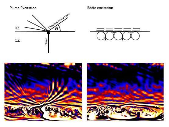
The convection in these simulations is dominated by convective plumes which emerge from the core and generally span the depth of the convection zone. Once the plumes impinge on the overlying stable region they become unstable as they are decelerated by the rapid variation in the Brunt-Vaisala frequency. As the plumes become unstable they break up into small eddies which propagate laterally along the convective-radiative interface. This behavior can be seen in the time snapshots shown in Figure 1 , although it is best seen in animation, which can be found www.solarphysicist.com. The destabilization of the plume and subsequent eddy production leads to substantial mixing and convective overshoot in the model.
Convective overshoot in massive stars has received much attention both theoretically and observationally (Roxburgh, 1965, 1992; Woo & Demarque, 2001). Such overshoot can lead to chemical mixing which could provide fuel from the radiative envelope into the convective core, thus extending the lifetime of the star. Although there are several ways to define the overshoot depth, here we define it as the first place the kinetic energy flux changes sign outside the convection zone. In Figure 2 we show the overshoot depth as a function of rotation rate (and time) for a subset of the uniformly rotating models. There we see that the overshoot depth varies substantially between Hp, where Hp is a pressure scale height (see figure caption for symbol distinction).
Although there are clear exceptions, in general, the overshoot depth decreases for increasing rotation rate and increases in time (later times denoted by diamonds). This occurs because radial motions are deflected azimuthally by the Coriolis force, thus limiting their ability to overshoot the convective-radiative interface. Indeed, we find that radial velocities at the interface are nearly 40% smaller in our highest rotating models, relative to our non-rotating models. This rotation rate dependence was also found in Brummell et al. (2002). We also note that the while the penetration depths increase in time, many of our models show saturation at later times.
Although more work needs to be done for various stellar types, our results indicate that there is a wide range of penetration depths that can be achieved in a given model, that the penetration depth can evolve in time and that the rotation rate can have an order 2 effect. It is interesting to note that the effectiveness of mixing by Eddington-Sweet type circulations (at a given age) increases with increasing rotation rates, whereas mixing by convective overshoot decreases with increasing rotation rate. These two effects may create a “sweet spot” in rotation space and age, where mixing beyond the convection zone is optimized.
In the above we measured convective overshoot, that is, how far convective motions could extend into the radiative zone, defined by the initial temperature stratification. As discussed in Zahn (1991) continual convective overshoot could transfer enough heat to the region to bring about a change in the mean thermal stratification, what is often referred to as “penetration”. We show the mean temperature stratification as a function of radius for several models in Figure 3 (see Figure caption for details). We see that models with lower rotation and/or differential rotation have, on average, more penetration.
In these models we see substantial convective overshoot and penetration, both of which depend on the rotation rate, with faster rotators showing lower penetration and overshoot. These results are consistent with observational constraints that place convective overshoot near 0.2-0.3Hp (Meynet et al., 1993), although our values may be on the high side due to slightly larger convective velocities (see Section 2 and Section 6). We note that because a shear flow is set up between the convective and radiative regions, and because the Brunt-Vaisala frequency is low near the interface, the overshoot region is unstable to shear instability. This would also cause substantial mixing in the region, but such mixing may or may not be relevant in the presence of convective overshoot and penetration.
4. Internal Gravity Wave Dynamics
4.1. Fundamentals of IGW and Wave-Driven Mean Flows
The simulations presented here are of inertial gravity waves, which have a simplified dispersion relation:
| (4) |
where is the frequency of the wave333Note that this dispersion relation is for an f-plane model, which is not the geometry of our simulation but it yields effectively the same dispersion relation assuming f=2., f is , are the horizontal and vertical wavelength, respectively, and N is the Brunt-Vaisala frequency. In the absence of rotation, this dispersion relation is often written as
| (5) |
where is the angle between the horizontal plane and lines of constant phase. Therefore, shallow angles imply a low frequency, while steep angles imply a high frequency. Another simplification of the dispersion relation can be found in the limit of , the dispersion relation then reduces to . For pure IGW, waves can only propagate when . When rotation is considered waves can only propagate when . Waves with frequencies approaching N are internally reflected, whereas waves with frequencies lower than the rotation frequency encounter critical layers, where most of the wave energy is dissipated.444A critical layer is defined as the position where the local angular velocity is equal to the horizontal phase speed of the wave. In the ray-tracing description of IGW the vertical wavenumber goes to infinity at a critical layer, and, therefore, the time to approach the critical layer goes to infinity. This means any small dissipation leads to complete, or nearly complete, absorption of the wave at the critical layer.
From the dispersion relation one can show that the phase velocity in the absence of rotation is
| (6) |
and the group velocity is
| (7) |
one can then see that the phase and group velocities are perpendicular, while the vertical components are in opposite directions (note that vectors are represented as (horizontal component, vertical component)). Therefore, if the group velocity is moving outward the phase velocity is moving inward and the fluid motions are along lines of constant phase. As a wave propagates outward from the convection zone the Brunt-Vaisala frequency is increasing, therefore, the ratio is decreasing, consequently the fluid motions and phase path are refracted, causing the wave motion to be a spiral path outward from the convection zone. It is worth noting that while stratification forces fluid motions to be more horizontal, rotation forces fluid motions to be more vertical, so that these two forces (buoyancy and Coriolis) have opposite effects on the fluid motions.
How these waves transport angular momentum has been a topic of intense research in the atmospheric science community. Here we review some of the basics of wave-driven mean flow (the interested reader is referred to standard atmospheric science textbooks, such as Pedlosky (2003); Holton (2004); Lindzen (1990)). When a single propagating wave is attenuated it transfers angular momentum to the mean flow (Eliassen & Palm, 1960). The forcing of the mean flow by waves depends on the wave attenuation, which depends on the frequency of the waves relative to the mean flow, which in turn, depends on the mean flow. Therefore, wave-mean flow dynamics is highly nonlinear.
One can appreciate how angular momentum is transferred from waves to the mean flow by considering the longitudinally-averaged horizontal component of the momentum equation (Holton, 2004; Lindzen, 1990):
| (8) |
where is the azimuthal velocity, and is the radial velocity and overlines denote a horizontal average. This equation shows that the mean zonal flow, , is driven by the divergence of the horizontally-averaged Reynolds stress and is decelerated by viscous dissipation.
The mean zonal flow maintained by internal gravity waves is typically depth dependent, i.e., a flow. This ”anti-diffusive” nature of gravity waves can be explained heuristically. Imagine a prograde wave (0) and a retrograde wave (0) excited at the same radius. If the medium in which the waves propagate is differentially rotating, these waves will be doppler shifted by:
| (9) |
Therefore, if the angular velocity, , of the medium increases in the direction of propagation, the prograde wave is Doppler shifted to lower frequency, whereas the retrograde wave is shifted to higher frequency. These frequency shifts are relative to the frequency at which the waves were generated, , where the angular velocity is .
Considering the simplest dissipation mechanism, radiative damping, the dissipation length goes approximately as where is the horizontal group velocity555Note, the vertical group velocity is often used here, but the wave propagation is predominantly horizontal, therefore, it is more realistic to use the horizontal group velocity (Rogers & MacGregor, 2011). Furthermore, we find both here, and in previous work, that an dependence which arises from considering the horizontal group velocity, fits the data from numerical simulations better than a dependence. and is the dissipation rate, . Using Equation (7) for the horizontal group velocity, we arrive at a dissipation length which depends on frequency and wavenumber like:
| (10) |
Therefore, waves which are dopper shifted to higher frequency (retrograde waves in the above example) will have a longer dissipation length than those shifted to lower frequency and therefore, will propagate a longer distance before being dissipated. Alternatively, the higher frequency wave will have a higher amplitude after traveling a set distance relative to the lower frequency wave.
A prograde wave transports positive angular momentum, whereas a retrograde wave transports negative angular momentum. Therefore, where a prograde wave is dissipated the mean zonal flow is accelerated and where a retrograde wave is dissipated the mean flow is decelerated. In this way two waves excited at a given radius with the same frequency and wavenumber but spiralling in opposite directions outward can lead to a radial shear flow. This process is self-reinforcing and so the shear will grow until viscosity becomes important. Plumb (1977) showed that two waves are unstable and will produce a shear, even in the absence of rotation or an initial shear. This was also demonstrated in the remarkable experiment by Plumb & McEwan (1978).
5. IGW Dynamics in Massive Star Simulations
5.1. Overview
Figure 1 shows the evolution of Models U2 and U8. In the following paragraphs we will briefly describe the wave-mean flow interaction that leads to the behavior shown in those figures with more details given in the subsequent sections (again, the interested reader is referred to the above texts or Buhler (2009), which discuss wave-mean flow interaction in great detail). Waves are generated at the convective-radiative interface and propagate into the radiative envelope toward the surface. Waves are generated both by direct plume incursion and by eddies propagating laterally along the interface. These processes produce a rather broad spectrum in frequency and wavenumber. The waves then propagate nearly horizontally in a spiral path outward due to the small ratio of and the variability of N with radius (see, for example, Figure 1 c,d,j).
As waves propagate toward the surface their amplitudes are affected primarily by two effects: radiative diffusion which acts to dissipate waves and density stratification, which acts to amplify waves. The combination of these two effects implies that the waves that make it to the surface of the star with the highest amplitude are primarily high frequency, large scale waves. These waves make it to the surface with high enough amplitude that they are subject to wave breaking and consequent angular momentum transfer. This angular momentum transfer drives a mean flow (seen as negative vorticity, black, in Figure 1b-e and positive vorticity, white, in Figure 1g-j).
In an initially uniformly rotating model the sense of the initial mean flow that develops (prograde or retrograde) is random (Plumb, 1977). In the models shown in Figure 1, U2 shows a mean flow at the surface, while U8 shows a mean flow at the surface. As waves propagate into a differentially rotating medium they are doppler shifted as described in Equation (9).
Considering the model U8 (bottom panel in Figure 1, bottom panel in Figure 14). Once the prograde mean flow develops, prograde waves propagating into that flow are shifted to lower frequencies and therefore, dissipated in shorter distances, while retrograde waves are shifted to higher frequencies and thus dissipated less strongly666Note that the waves are dissipated continuously and the dissipation length is just defined in the normal sense of when the amplitude has decreased by a factor of e.. The prograde waves deposit positive angular momentum thus causing the prograde shear flow to in time. As the shear grows, the differential rotation increases, and prograde waves are shifted to lower and lower frequencies, and therefore, dissipated in shorter and shorter distances, causing the mean flow to migrate toward the source of the waves in time (note the difference in the extent of the mean flow between Figure 1b and d, or g and j). Therefore, this process is self-reinforcing, until viscosity becomes relevant.
As the entire region is spun up, angular momentum must be conserved and therefore, the convecting core slows down. This configuration, in which the angular velocity is increasing outwards allows retrograde waves to now reach the surface with higher amplitude than their prograde counterparts. This leads to transport of predominantly angular momentum and the consequent slowing of the outer regions, eventually leading to a reversal of the mean flow at the surface (see Figure 14).777We have not been able to model a full reversal at this time due to an instability which develops in the flow. This instability is currently under investigation.
The wave-mean flow interaction described above has been elucidated well in many text books, and was first described by Holton & Lindzen (1972) to explain the Quasi-Biennial Oscillation of the Earth’s equatorial stratosphere. The process was then demonstrated in the remarkable experiment by Plumb & McEwan (1978). What we observe in our simulations is not a new physical process, it is only the application of this physical process to massive stars.
5.2. Wave Generation
The generation of waves at convective-radiative interfaces has received much attention in stellar physics as it is the amplitude and spectra of waves generated that dictates the details of angular momentum transport and mixing by these waves. The work of Press (1981) and Garcia-Lopez & Spruit (1991) use physical arguments matching the ram pressure of the convective fluctuations to the wave pressure, combined with a Kolmogorov spectrum of turbulence to arrive at a wave spectra. Work by Kumar et al. (1999); Montalbán & Schatzman (2000a); Lecoanet & Quataert (2012) solve an inhomogeneous wave equation with a source term to represent the wave driving. The source term in those models takes the form of Reynolds stresses provided by convective eddies, as in Kumar et al. (1999); Lecoanet & Quataert (2012) or that of a plume model as in Townsend (1966); Montalbán & Schatzman (2000a). Not surprisingly, the various models lead to different spectra. For example, the model of Kumar et al. (1999); Lecoanet & Quataert (2012) in which the source term is that of convective eddies leads to spectra of the form:
| (11) |
where and b=2. This models shows that ) is a decreasing function of frequency and a function of scale which increases at low wavenumber to some typical length scale and then decreases at higher wavenumber. The plume model of Townsend (1966); Montalbán & Schatzman (2000a) leads to a wave energy spectrum of the form:
| (12) |
in which is the characteristic timescale of plume intrusion and is a characteristic spatial scale. In this model decreases exponentially with frequency and scale.
Besides the obvious differences in these spectra there is also a more qualitative difference in the frequencies and scales thought to be associated with the different processes of plume excitation and convective eddie excitation. In the plume theory the frequencies are associated with the timescale of plume intrusion. Given the steep gradient of the Brunt-Vaisala frequency, the plume is halted shortly after entering the radiative region and therefore, plumes can drive high frequency waves. The typical wavelength is associated with the horizontal extent of the plume. Given the thin-ness of the plume this would indicate small horizontal scales (although see discussion below). On the other hand, convective eddies that span some fraction of a pressure scale height and have slower turnover times would drive larger scale waves and shorter frequencies. Therefore, in the theories described above, convective eddies are responsible for low frequency, large (horizontal) wavelength waves, while plumes are associated with high frequency, short wavelength waves.
Turning to our simulations we can get a qualitiative picture of the wave generation process (again, although images are shown here, the clearest picture of the physical processes can be seen in animation at www.solarphysicist.com). The convection zone is dominated by plumes which span the extent of the convective core, often impeding on the overlying convection zone. As the plume intrudes into the stable region it is rapidly decelerated by buoyancy causing the plume to break up, generating laterally propagating vortices at the interface which are a fraction of the convection zone depth. Therefore, both plumes and eddies contribute to the spectrum of wave energy.
Wave generation by each of these processes can be understood qualitatively. As plumes intrude on the overlying convection zone they drive waves with wavelengths similar to the plume intrusion depth (which is small, see Figure 4), this gives rise to large horizontal scale waves, since where are the vertical and horizontal length scales. In animation, and figures, plume intrusions can clearly be associated with large horizontal scale waves. On the other hand, shorter wavelength waves are seen to be driven as the plume breaks up into laterally propagting small scale eddies. Qualitatively, this means plumes are associated with large scales, while eddies are associated with small scales.
The frequency of waves generated by the plume incursion can be seen in Figure 4. When the plume intrudes, there are a variety angles of phase lines with respect to the horizontal that are generated, indicating plumes generate a variety of frequencies (see Figure 4 left panels). In the dispersion relation for IGW expressed in Equation (5), the angle is the angle between the horizontal and lines of constant phase. Therefore, shallow angles indicate low frequencies, while steep angles indicate higher frequencies. On the other hand, when there are no plume incursions waves are driven by stresses provided by convective eddies (see Figure 4 right panels).
We can evaluate the wave spectrum more quantitatively by looking at the wave energy as a function of frequency and wavenumber. Because our numerical code is spectrally decomposed in the horizontal dimension this can be done easily by taking a fourier transform of a time series of data at a particular radius. The results of this procedure are shown in Figure 5, at different radii at both early and late times. In Figure 5 we see that at the convective-radiative interface, waves are generated with a broad spectrum down to horizontal wavelengths of cm () and up to frequencies of . Moving into the bulk of the radiative envelope we see that lower frequency waves have been dissipated and we see ridges in the power spectrum, indicative of standing g-modes. Finally, at the surface we see only fairly high frequency waves.
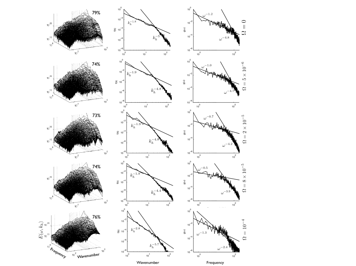
In this section we address the spectrum and amplitudes of wave generation at the convective-radiative interface and leave the issue of their propagation and attenuation with radius for the next sections. Therefore we concentrate on the energy spectrum shown in the bottom panels of Figure 5. In Figure 6 we show the wave888The word “wave” here is used loosely and only means horizontal wavenumber not equal to zero, these ”motions” do not necessarily obey a simple, linear dispersion relation. spectra as a function of frequency and wavenumber at 0.5 pressure scale heights above the convective-radiative interface for several of our models with varying rotation rate (see Figure and caption for details). One can see that waves are excited at all frequencies and wave numbers but the amplitudes fall off rapidly at high wavenumber (small scales) and high frequencies as predicted in both the theories described above.
By inspection one might expect that the energy shown in the left panels of Figure 6 is a separable function in frequency and wavenumber and we indeed confirm that this is the case using a singular value decomposition (SVD) of the wave energy. We find that a separable function can explain of order 70-80% of the power seen in Figure 6, as denoted by the percentages shown in that Figure999Moving further into the radiative interior the function becomes less separable, as expected given that the dispersion relation strongly links frequencies and wavenumbers.. Assuming the wave energy can be written as the separated function
| (13) |
where and come from the SVD, we find that the best fit solutions to the data are power laws, as shown in the middle and right panels of Figure 6, respectively. We generally find that the wave energy can be approximated well as , with both wavenumber and frequency spectra fit best by two separate power laws. We find that at low frequencies and at high frequencies is . Similarly, at low wavenumbers and at high wave numbers (smaller scales) . The mean and standard deviations are calculated from all our models in which the heat flux is the same (Models U1-U9 and D10-D14). Within a given model there is also variation in power law spectra in time. When sampled at 12 non-overlapping times, model D11 shows at low frequencies and at high frequencies, at large scales and at small scales. Where the mean and standard deviations quoted refers to the variation in the spectra over these 12 times. From these values we deduce that time variation of a spectra is stronger than variations due to rotation. However, we note that the trend in power laws in both frequency and wavenumber is always seen. We expect that these two power laws are associated with the two different processes of plume and eddie excitation, at least broadly.
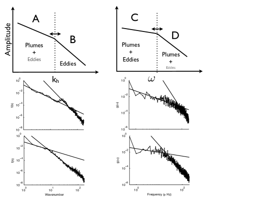
Figure 7 shows a diagram of which processes we think dominate which region of the spectrum seen in Figure 6. Large horizontal length scales, Region A, are dominated by plumes, with eddies contributing to a lesser extent by the coherent sum of many waves. As described above, the vertical wavelength of a plume is related to the plume intrusion depth. This length scale is short, therefore, with the approximate dispersion relation given by , is therefore, larger than the vertical length scale by the amount . If the vertical wavelength is the penetration depth, , then the horizontal wavelength is given by . Therefore, the minimum horizontal wavelength is , hence the maximum horizontal wavenumber associated with plumes is approximately the wavenumber associated with the penetration depth. From Section 3, the penetration depth varies from , which corresponds well to a horizontal wavenumber of 15-30, approximately the horizontal wavenumber at which we see a break in slope in Figure 6. This also explains why there is a time variation in the break point between the slopes: at different times plumes penetrate greater or lesser distances and are present to greater or lesser extent hence, smaller and larger horizontal wavenumbers where the spectral slopes change. Since plumes likely do not penetrate much further than the penetration depth they likely dont contribute much to the smaller scales of Region B. Therefore, those waves must be predominantly driven by eddies at the interface.
We have seen in Figure 4 that eddies and plumes generate low frequency (low phase angle) waves. Hence, Region C has contributions from both plumes and eddies. On the other hand, in that same figure, and in animation, we see that plumes are dominantly responsible for high frequency (high phase angle) waves. The break in slope in the frequency spectrum occurs over a broad range . If eddies are assumed to have length scales of and speeds of , then the typical eddy frequency is . We observe eddies generated at the interface to have length scales of and speeds in the range of cm s-1, the frequency associated with such eddies is Hz, allowing for variations in speeds and eddie size, we gather that turbulent eddies can generate frequencies up to approximately this value, give or take a factor of a few. We see the upper end of this range is near the break point frequencies seen in Figure 6 and Figure 4.
On the other hand, if we assume plume frequencies are associated with the typical time of a plume incursion, plume frequencies can be estimated as , where are plume velocities, typically a few times larger than the eddie velocities. With the penetration depths given in Section 3, we find frequencies in the range of 80-500Hz. The lower end of this range is similar to the position of the break points in frequency. Note that both of these frequencies are proportional to some velocity at the convective-radiative interface, and that these velocities decrease with increasing rotation rate. This may explain why the break point in the frequency spectrum moves to lower frequencies for higher rotation rates.
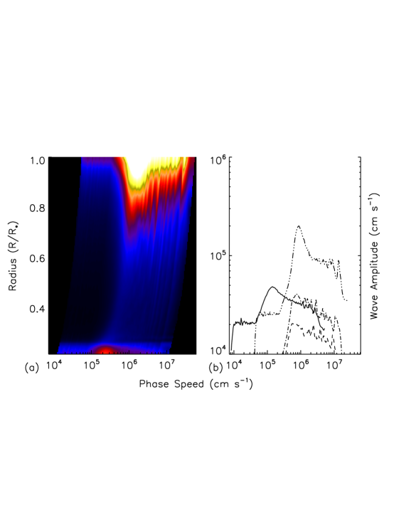
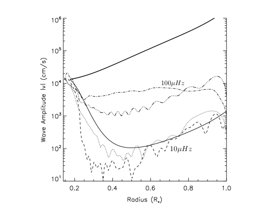
Another way to investigate the wave generation process is to consider the amplitudes of waves generated as a function of phase speed rather than as a function of frequency and wavenumber individually. This is shown in Figure 8. There we see that IGW are generated in a very narrow range of horizontal phase speeds from cm , with a sharp cutoff at lower phase speeds and a gradual decline at higher phase speeds. In Figure 8 we show the velocity amplitude, which shows the same behavior as in Figure 10, with amplitude initially large, then decreasing throughout the bulk of the radiative envelope and finally increasing again toward the surface. This is distinctly different than the energy which would decrease strictly in radius. Moving outward into the radiative envelope we see that the peak velocity amplitude occurs at higher and higher phase speeds. This is the result of both dissipation of the lower phase speed waves, as well as energy transfer to higher frequency waves (see Section 5.4). While the energy is predominantly in propagating IGW we also see peaks at distinct phase speeds in Figure 8b indicative of the standing g-mode component.
It is noteworthy that the phase speed at which waves are predominantly generated is nearly identical to the dominant radial velocity at the interface (105-106 cm). While the frequency and wavenumber spectra of generated waves is broad, the phase speed spectrum is relatively narrow. Given the frequency and wavenumber spectrum generated we could have seen a range of phase speeds between cm s-1, yet we find a much narrower range over which energy is generated.
Another important quantity associated with wave generation is the total flux delivered from the convecting region to waves. This is typically measured by the quantity:
| (14) |
which refers to the wave energy flux as derived in Lighthill (1978) where p’ is the pressure fluctuation and is the velocity. We show this quantity as a function of radius for a number of our models in Figure 9 (see caption for details). It has been predicted in several studies (Goldreich & Kumar, 1990; Kumar et al., 1999; Lecoanet & Quataert, 2012; Shiode et al., 2012) that the integrated wave flux is
| (15) |
where is the convective Mach number and is the convective flux. The typical radial velocities at the convective-radiative interface are cm s-1 with intermittent excursions to much larger values. The sound speed at the interface is 5 107 cm s-1, therefore, the convective Mach number is . The total flux at the convective-radiative interface is ergs cm-2s-1, from Figure 9 we see that the wave flux there is ergs cm-2 s-1, so the ratio of wave flux to total flux is , but can be larger. This is generally consistent with the theoretical prediction encapsulated in Equation (15).
In summary, we find that the spectrum of waves generated by overshooting convection is broad, but generally with a decreasing function of frequency and wavenumber. Although we attempted many functional fits to this data, we find that combined power laws fit the data the best. We see breaks in the power law fits in both frequency and wavenumber, which could be attributed to the different physical processes of wave generation by impeding plumes and convective eddies at the interface. These spectra are substantially different than those predicted by the theories described in the Introduction. When one considers our “low” frequencies which generally span up to around 60-80 the power law is , substantially less steep than the -4 - -6.5 power law predicted by Kumar et al. (1999) and Lecoanet & Quataert (2012). Similarly, for our “low” wavenumbers which include wavenumbers out to 15-30, the slope is , also substantially different than that predicted. This is likely due to a number of effects, most fundamentally that we include the effects of both impinging plumes and eddie generation and that these generation processes interact with each other, as do the waves they generate. This interaction would likely lead to a flatter spectra, such as the one we produce. While the total wave flux is consistent with previous theoretical predictions our wave energy is distributed more broadly in frequency and scale, showing less severe drops in energy at higher frequency and wavenumber than previous analytic predictions. Possibly more fundamentally, rather than matching frequency and scale of convection individually we find that waves are generated in a narrow range of phase speed, which corresponds to the radial velocity of convective motions at the interface. It is likely that these spectra will change somewhat in three dimensions (3D). The third dimension may provide another avenue for transfer of energy to smaller scales and therefore, allow for a steeper spectrum than the one we see here. Probably more fundamentally, it is likely that the nature of the turbulence and plume dynamics changes. It is difficult to say how these changes will affect the wave spectra.
Until 3D numerical simulations of wave excitation can be done it might be possible to learn something from experiments of IGW driven by plumes and convection. Several experiments of turbulence and plume driven waves have been conducted (Ansong & Sutherland, 2010; Holdsworth et al., 2012) and have found that these processes generate waves in a narrow range of frequency, . The physical reason for this narrow range is still unknown, although the authors note that these values of the frequency are optimal for transporting horizontal momentum vertically and speculate that there is a nonlinear interaction between the driving region and wave propagation region in order to bring about maximum angular momentum transport. If this is true, it would imply that the simple theories of wave excitation discussed in the introduction are inadequate as they completely neglect any wave influence on the convection. More recent experiments of convectively driven IGW are being carried out by M. LeBars at the SpinLab at UCLA, preliminary results show a power law in frequency similar to those found in our simulations (private communication), however more quantitative comparisons await more complete data from the experiments. How these experimental results extend to stars with a rapidly varying Brunt-Vaisala frequency is unknown.
5.3. Wave Propagation
Once generated at the convective-radiative interface, IGW propagate toward the stellar surface. As discussed in Section 5.1 the wave propagation is outward, along spiral paths, with the angle of phase lines with respect to the horizontal set by the ratio of . As waves propagate toward the surface their amplitudes are affected by two main effects, radiative dissipation and conservation of pseudo-momentum. By conservation of pseudo momentum , the wave amplitude increases like . In these models the density decreases from approximately 30 gm cm-3 at the top of the convection zone to gm cm-3 at the top of the radiation zone, so one would expect the wave amplitudes to increase by nearly two orders of magnitude. This acts on all waves, regardless of frequency and wavenumber.
Second, waves are radiatively dissipated. Because gravity waves are thermal perturbations they are subject to radiative dissipation. The wave amplitude, acted on by the combined action of density stratification and radiative dissipation can be written as:
| (16) |
where
| (17) |
where is the radius at the interface and is the wave amplitude at the interface. By Equation (17) radiative dissipation is most effective at dissipating low frequency, high wavenumber (small scale) waves. Which can be physically understood as short wavelengths have high curvature and are therefore, dissipated rapidly. Similarly, short frequencies have a longer time over which to feel the effects of dissipation. Alternatively, using the relationship , the integrand in Equation (17) can be rewritten as and one can see that waves with short vertical wavelength are dissipated more efficiently.
These two effects on the propagation of IGW are the most fundamental. Clearly, in massive stars where the waves propagate into regions of decreasing density, density stratification and radiative dissipation have opposite effects. Figure 10 shows these combined effects for a couple of frequency and wavenumber combinations, which was found by integrating Equations (16) and (17) above using the thermal diffusivity set in the simulation and the Brunt-Vaisala frequency from the stellar model, yet using amplitudes at the interface given by the simulation (solid lines). Also, shown in that figure are the amplitudes of waves, as a function of radius, from our numerical results for the same frequency/wavenumber combinations (broken lines, easily discerned as waves, whereas the model shows straight lines). There we see that low frequency waves are dissipated similar to predictions, while high frequency waves are dissipated more than theoretical predictions, with some dependence on scale. The discrepancy between the theoretical prediction and numerical simulations is more severe for the lowest frequencies and smallest scales. Theoretically those waves would have virtually no amplitude at the surface, while the numerical simulations show amplitudes similar to those shown in Figure 10 for higher frequencies and lower wavenumbers. Overall, the numerical simulations show far less dispersion between wave amplitudes of different frequencies and wave numbers than the simple theory would predict. The difference between the predicted behavior and that seen in the simulations is likely due to nonlinear effects such as wave-wave interaction, wave-breaking or wave-mean flow interaction (see Section 5.4).
Figure 11 shows the surface velocities for a subset of our models and for a variety of frequency/wavenumber combinations (see figure caption for details). We often see waves which are nearly (but not quite) a km/s. The large triangles represent the maximum velocities obtained during the times we investigated. These maxima are associated with higher frequency, smaller scale waves. This is not quite in the range of the non-thermal surface velocities needed to explain macroturbulence (Aerts et al., 2009), but considering the enhanced diffusivity and viscosity in these simulations, it is possible to imagine IGW potentially contributing to the “macroturbulence” necessary to explain spectral line widths (Howarth et al., 1997).
Recently, (Shiode et al., 2012) have investigated the detectability of IGW in massive stars by the spacecraft mission Kepler. In that study the emphasis is on g-modes, the waves which form a standing pattern between the surface and convective-radiative interface. The waves most likely observable would be those of the largest scale. We show large scale waves () of frequencies 10Hz, as diamonds and squares, respectively, in Figure 11. There we see that these waves have much lower amplitudes than the maximum values, ranging from cm/s. These amplitudes are approximately an order of magnitude larger than those predicted by Shiode et al. (2012). There are several likely reasons for this discrepancy. First, in our simulations high frequency waves are excited directly by plumes, with fairly high amplitude, rather than relying on the incoherent addition of multiple eddie sources. Second, Shiode et al. (2012) only consider standing waves while our waves likely have a propagating and standing component (as seen in Figure 5). Finally, as discussed in Section 2, we have a larger luminosity than an actual star of this size, this results in a larger velocity within the convection zone, although we believe this is offset by enhanced diffusion (see Section 6).
5.4. Wave-Mean Flow Interaction
As shown by Eliassen & Palm (1960) IGW can only transport angular momentum if they are attenuated. Typical attenuation mechanisms include radiative diffusion, wave breaking at critical layers or large amplitude wave breaking. In practice it is difficult to ascertain which dissipation mechanism is at work under various circumstances.
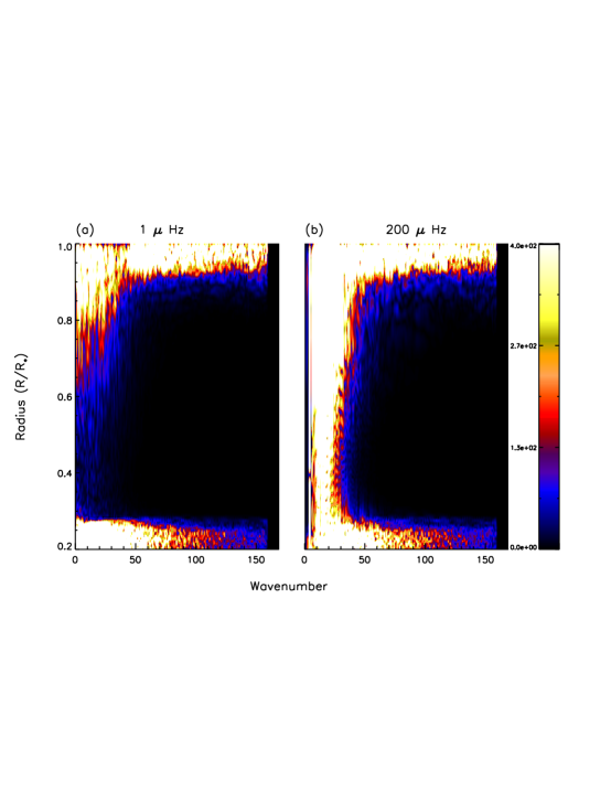
We discussed the effects of radiative dissipation in the previous section and here we turn to critical layer absorption and wave breaking. Figure 12 shows the wave amplitude as a function of wavenumber and radius for both high and low frequencies. What we see is that wave generation is dominated by low wavenumbers (, as also shown above in Figure 5 and in Section 5.2). We see that only the largest scales and highest frequencies have appreciable amplitude within the bulk of the radiative envelope but that near the surface high amplitudes are seen even for small scales and low frequencies. Furthermore, for the smallest scales the amplitudes at the surface are larger than they were at generation. This implies generation of small scale waves at both low and high frequencies. Transfer of energy from large scales to small scales occurs both during wave breaking as well as when waves encounter critical layers (Rogers et al., 2008).
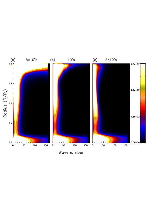
If we look at the same plot, but at various times, integrated in frequency, as in Figure 13, we can distinguish between critical layers and typical high amplitude wave breaking. In Figure 13a we see that there is substantial energy at small scales at the surface. This time is sufficiently early that a strong mean flow has not yet developed and there is, as yet, no critical layer (Figure 14). Therefore the energy at smaller scales is most likely due to high amplitude wave breaking. Figure 13b represents a time around when the critical layer is forming (also see Figure 14). At this time energy is still being transferred to small scales by wave breaking but some of that small scale energy is being absorbed into the critical layer (smaller scale waves have smaller phase speeds and are therefore, more susceptible to critical layer absorption). Figure 13c shows the wave energy after the mean flow has developed, we see that there is only energy in the largest scales (probably predominantly in standing g-modes). Energy in smaller scale waves, that was generated by wave breaking is now being absorbed by the critical layer. Note that once the critical layer develops the linear velocity at the surface is on the order of cm s-1, precisely equal to the phase speed where IGW are peaked at the surface (Figure 8).
The wave-mean flow interaction we have described above is very complex. It involves both wave breaking and critical layer absorption, the development of a mean flow which then alters the properties and propagation of the waves and the subsequent evolution of the mean flow. This all occurs from the propagation and interaction of a broad spectrum of convectively generated waves in a highly stratified gas.
5.5. Angular Momentum Transport
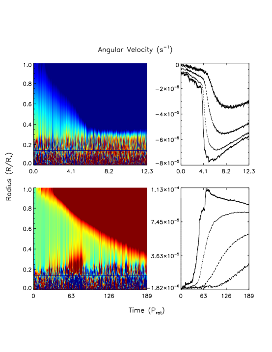
In Figure 14 we show the angular velocity over time for three of our models (U2 (top) and U8 (bottom)). There we see, as described above, a mean flow develops first at the stellar surface. Over time the angular velocity migrates toward the source of the waves (the convection zone) in time. As it does so the convection zone starts to spin predominantly with the opposite sense, in order to accomodate angular momentum conservation. We see that the most rapidly rotating model, U8, achieves a higher absolute angular velocity at the surface. In general, we find that the extreme angular velocities seen in Figure 14 bracket the maximum values achieved in our models and that the trend is for faster rotators to achieve slightly higher mean flow amplitudes. This is not a strong effect as a factor of 100 increase in rotation leads to an 40% increase in angular velocity.
One will notice that the modulation of angular velocity in time is not symmetric. The growth is initially dominated by critical layer absorption, which causes a rapid increase in angular velocity. Once the angular velocity is saturated, the amplitude is so large that it is not critical to many waves, so the decay is much slower, being dictated by a weaker effective wave flux and viscous dissipation of the mean flow.
The mean angular momentum transport by IGW is described by Equation (8), is often referred to as the wave flux and the second term on the left hand side of Equation (8) is the acceleration of the mean flow due to waves, we refer to it as wave acceleration.101010Viscous diffusion terms are negligible most of the time and at most locations. In Figure 15 we show the time average of the wave acceleration as a function of radius for several of our models. There we see that wave acceleration is substantial both near the base and at the top of the radiative envelope. With accelerations nearing 0.1-1 cm s-2 the linear (and angular) velocity at the surface can change dramatically on relatively short timescales. For example, with this acceleration, an initially non-rotating star can achieve surface angular velocities of 10-5 -10-4 rad s-1 in a few years. This is consistent with the accelerations seen in Figure 14.
Upon inspection of Figure 14 one will see that angular velocities increase by a factor 10 in a few rotation periods (depending on the model). The angular velocities attained are a function of the wave flux, which itself is a function of the convective flux, set by nuclear energy generation. In our simulations the convective flux is larger than the stellar convective flux by a factor to offset our larger than stellar thermal diffusivity. By mixing length theory this would lead to velocities which are 30 larger than stellar convective velocities. If these velocities were not offset by the larger than stellar diffusivities, then the wave flux, as described above would be 1000 too large. Dunkerton (1981) has argued that the period of oscillation is inversely proportional to the wave flux.111111Plumb (1977) argued that the period of oscillation was inversely proportional to the product of the wave flux and damping rate. However, this was for Boussinesq systems. In compressible systems Dunkerton (1981) argued, and his compressible simulations confirmed, that there was very little dependence on the damping rate. Rogers et al. (2008) also saw little variation in oscillation period with the thermal diffusivity. Using this scaling, our periods of modulation are too short by a factor of 1000. Therefore, if we apply this scaling we arrive at a modulation time of a few-10000 rotation periods. For our fast rotators this results in modulation times of 10-30 years. This estimate comes with some caution. First, it is difficult to estimate how much the wave fluxes are enhanced. We believe that our large wave driving is offset by our large wave damping, so a factor of 1000 is likely an overestimate. Second, the scaling of the period of oscillation has come from simplified models with few waves and no critical layers. Finally, the timescale for modulation will depend on the phase in which one is observing. During the critical layer growth phase, variations occur much more rapidly, so one may see variation in a few years. However, during the decay phase, when no critical layers are present and net wave fluxes are low, modulation may occur on a longer timescale.
6. Dependencies
Wave generation, propagation, dissipation and consequent angular momentum transport could depend on the parameters of our simulations. In this section we discuss how various parameters affect the most important aspects of our results: spectra of wave generation including amplitudes and consequent angular momentum transport. We will also discuss other dependencies, such as convective velocities and convective overshoot as they pertain to the wave spectra and angular momentum transport.
6.1. Rotation
We see in Figure 6 that the wave spectra varies some with rotation rate. In general, these variations are not larger than variations within a given model in time. However, there are a couple of clear trends. First, the low frequency wave spectra are flatter as the rotation rate is increased. This occurs because higher rotation rates allow for larger differential rotation. Larger differential rotation leads to larger doppler shifts of wave frequencies, and therefore, a larger range of wave frequencies, particularly at low frequencies. This gives rise to a flatter spectrum at lower frequencies. This is also true at higher frequencies, but higher frequencies are shifted less, relative to their fiducial frequency, so the effect is weaker, as is seen in the spectra. Second, the frequency at which the slopes of the spectra change tends to be lower for higher rotation rates. This is likely because radial velocities are decreased in rapidly rotating models. Since radial velocity is directly related to the plume intrusion depth, this affects the frequencies of waves generated by plumes and hence, the break point frequency. This also explains the shift in wavenumber spectra.
At our highest rotation rates, the rotation frequency is . This is very similar to the frequency at which we see a pile up of wave energy. This behaviour has been seen in experiments as well (Holdsworth et al., 2012). The Rossby number which is a measure of the inertial terms to the rotation terms is defined as
| (18) |
where R is the radius at the interface, is a typical radial velocity at the interface and the other variables as defined above, we see that our fastest rotation rate corresponds to a Rossby number of . This is the only model of ours for which the Rossby number is lower than 1, indicating the Coriolis forces dominate the inertial forces. This may be why this is the only model to show a distinct buildup at the inertial frequency. It may also be because this is the only model for which the inertial frequency is at a high enough frequency to not be overwhelmed by low frequency waves driven by plumes and eddies.
We also find that, on average, wave amplitudes, mean flows and wave acceleration are all slightly larger in models with rapid rotation than in more slowly rotating models. The energy equation is the same in a rotating model, as the Coriolis force does no work. However, in rotating systems, energy is not partitioned equally between kinetic energy and potential energy (due to stratification). In rotating systems, more of the total energy is in the form of kinetic energy. In fact, the ratio of kinetic energy to potential energy is directly related to the rotation rate (Gill, 1982)
| (19) |
this means that in rotating systems wave velocities can be larger than their non-rotating counterparts at the expense of potential energy in the stratification. This effect is small, but it is noticeable and explains the small variations seen in wave amplitudes, wave acceleration and resulting mean flow.
6.2. Differential Rotation
There is little variation with any parameters when differential rotation is considered. We find a slight variation in penetration depth, as to be expected, as differential rotation produces a Kelvin-Helmholtz instability causing additional mixing. For differentially rotating models the spectra are more consistent and slightly flatter in frequency and smaller scales. This is consistent with these models being slightly more turbulent in the overshoot region due to shear instability. However, overall the variation between these models and the initially uniformly rotating models is not substantial compared to the overall variation of spectra in time and with rotation rate. Models with large differential rotation develop strong mean flows, while the one model with weak initial differential rotation does not, so it is likely that initially differentially rotating models develop strong mean flows more readily and that those flows have a preferential sense. Overall, the differentially rotating models are similar to those with no initial differential rotation.
6.3. Diffusivities and Heat Flux
Besides rotation, the other tunable parameters are the thermal diffusivty, the viscous diffusivity, and the heat flux, (or convective driving). Taken together these numbers, in the appropriate non-dimensional form, constitute the Rayleigh number:
| (20) |
which dictates the details of the convection, but does not necessarily dictate angular momentum transport by IGW. Regardless, we would like this number to be large to adequately represent turbulent motion within the convection zone. From the values listed in Table 1, we see that all of our models have extremely high Rayleigh numbers ( by this definition), except possibly model MU1-4.
Another control parameter that affects convection (and possibly waves) is the Prandtl number (Pr=). In stellar interiors this number is substantially smaller than 1 (). Unfortunately, these values are unobtainable in numerical simulations, especially while maintaining large Rayleigh numbers. Nearly all of our simulations have Pr larger than 1, except model MU1-4. In that model we achieve a Pr less than 1 by increasing , but this leads to extremely laminar flows (the Rayleigh number is reduced) which we think are less realistic than our turbulent flows with inaccurate Prandtl numbers. We argue that as long as our viscous dissipation is low enough to not dominate the momentum equation proper dynamics are recovered.
While the above parameters dictate the details of convection, what we are primarily concerned with here is what parameters affect the wave dynamics. Like convection, we expect all of these parameters to affect waves and wave driven momentum transport. Precisely how these parameters affect this transport is what we address here. First, convective forcing, in the form of , determines the velocities within the convection zone and therefore, it affects the vigour of convection (the Rayleigh number). Second, the thermal diffusivity dictates the diffusion of waves in their propagation to the surface and therefore, affects wave amplitudes and momentum transport. Finally, the viscous diffusivity affects the mean flow evolution.
We first address the spectra of waves generated. The mean spectral slopes of the modified models are (neglecting model MU1-3) for low frequencies and for high frequencies and at large scales and at small scales. These slopes are very similar to that of model U1 and certainly no more exceptional than the time variation within that model. Therefore, we conclude that none of these parameters affect the spectra much, with the exception of model MU1-3. In that model, the thermal diffusivity is so high that it dominates buoyancy and therefore, dissipates waves extremely efficiently, leading to steep slopes in the wavenumber spectra. Model MU1-2 which has a slightly lower thermal diffusivity shows virtually no difference in spectral slope (compared to the fiducial model U1). While it is possible that substantially lower thermal diffusivities could lead to flatter spectra, we expect (hope) that we have achieved large enough Rayleigh numbers that the buoyancy forces dominate diffusion enough so that the spectra remains relatively unchanged, this is somewhat validated with MU1-2. However, when we increase enough (MU1-3) this no longer becomes valid and the spectra changes drastically.
It is difficult to measure how much Q, and affect the surface amplitudes of the waves beyond basic qualitative understanding. Comparing the amplitudes of the largest scale waves () and frequencies of 10Hz of models U1 with MU1-2 (which we expect should have similar velocities if our scaling described in Section 2 is accurate), we find that on average the velocities are similar (average radial velocity for U1 is 290 cm s-1, while for MU1-2 it is 240 cm s-1). However, we note that both models vary substantially (by as much as an order of magnitude) over the extent of the simulation. This isnt too surprising given the variation in the mean flow and its ability to absorb wave energy. The time variation of the mean flow, and its affect on wave amplitudes makes direct comparisons difficult. However, we note that, on average, MU1-1, MU1-3 and MU1-4 all have lower velocity amplitudes at the surface compared to U1, while MU1-6 which has a lower Q and a similarly lower has higher velocity amplitudes (by a nontrivial margin).
When there is sufficient driving to offset dissipation, the slopes of the spectra as shown in Table 1 depend primarily on the time and spatial correlations of waves. However momentum transport by waves depends on a combination of the wave driving amplitude (the convection, ) and how those waves are dissipated during their propagation. Most fundamentally, it must be recognized that in order for a mean flow to develop the wave acceleration must be larger than the viscous diffusion (Equation 8), so reductions in and increases in if sufficiently large could lead to wave accelerations which are too small compared to the viscous dissipation to allow a mean flow to develop. This is just a statement that, in order for a mean flow to develop, the local Reynolds number must be greater than 1. This is most certainly the case in stellar interiors. Even with conservative estimates of wave speeds and scales (Shiode et al., 2012) the Reynolds number at the stellar surface should be substantially larger than 1 (assuming viscosities of order gives Reynolds numbers of ) . However, in numerical simulations this parameter space is difficult to achieve.
Given the velocities and scales seen in Figure 11 (squares and diamonds) combined with the viscous diffusivity listed in Table 1, the Reynolds number in our standard simulations (“U” and “D” models) is 1-10. Therefore, any reduction in , increase in or is likely to shut off mean flow acceleration. Indeed we find this is the case, as models MU1-1-MU1-5 all show decreased Reynolds numbers and (substantial) mean flows do not appear within the (rather long) time we ran the simulations. However, model MU1-6 which has reduced driving (), but similarly reduced (hence, the Reynolds number should still be 1) does show mean flow acceleration.
7. Discussion
These results have many theoretical and observational consequences, a few of which we discuss here.
1) Misalignment of Hot Jupiters around Hot Stars observations have important implications on the origin of these hot Jupiters, especially since a modest fraction of them show signs of significant obliquity angle . At face value, this observation would disfavor the disk-migration scenario compared to a dynamical mechanism for the origin of hot Jupiters. However, hot Jupiters with high are primarily found around stars with effective temperature () hotter than 6,250K (Winn et al., 2010), while the orbits of hot Jupiters around relatively cool, solar-like, stars are generally aligned with their hosts (Winn et al., 2010; Schlaufman, 2010).
Several dynamical mechanisms including Kozai resonances, planetary encounters, and secular chaos have been suggested as possible causes for the excitation of extra solar planets’ obliquity and eccentricity (Fabrycky & Tremaine, 2007). However, these processes do not explicitly depend on the mass of the star, . Therefore, Albrecht et al. (2012a) have suggested the following scenario leading to misalignment: 1) hot Jupiters around all stars attained a random obliquity distribution when they relocated to stellar proximity under one of the dynamical mechanisms discussed above, 2) their obliquities then evolved through tidal dissipation, on a time scale , and 3) the tidal dissipation timescale is shorter in cool stars because of their convective envelopes, thus is correlated with stellar type because planets around cool stars have had time to align through tidal dissipation, while planets around hot stars have not.
The above interpretation is based on the application of a model of the stellar tide by Zahn (1977), the quantitative details of which remain uncertain (Ogilvie & Lin, 2007; Goodman & Lackner, 2009; Barker & Ogilvie, 2010). If one resorts to the equilibrium tide for dissipation of obliquity, as in Albrecht et al. (2012b), the semi-major axis is simultaneously damped and the planets will fall into their host stars. On the other hand, if one relies on the dynamical tide introduced by Lai (2012) then planets evolve to aligned or anti-aligned systems, contrary to observations. Therefore, there currently appears to be no tidal mechanism which can explain the observations (Rogers & Lin, 2013).
Several other scenarios have been suggested as potential causes for the observed obliquity misalignment that are still consistent with the disk migration scenario. They can be categorized in terms of reorientation of either the protoplanets’ natal disks (Bate, 2010; Lai et al., 2011; Batygin, 2012) or the stellar spin (Rogers et al., 2012). For example, the spin orientation of protostellar disks may re-orient episodically, especially during the disk formation (Bate, 2010). If the host stars’ spin and the planets’ natal disks’ angular momentum vector are not initially parallel, an induced magnetic field (due to the interaction between stellar magnetosphere and the disk) could introduce a torque which will have the tendency to amplify the misalignment (Lai et al., 2011). In general, the “tilted-disk” scenarios do not provide obvious explanations for the observed correlation between obliquity and stellar mass. In contrast, the “stellar spin modulation” scenario described here and in Rogers et al. (2012) relies on the angular momentum redistribution due to the excitation, propagation, and dissipation of IGW. These processes are only effective in intermediate and massive stars with convective cores and radiative envelopes.
Based on the results presented in the previous sections, we anticipate the following observable tests of “stellar spin modulation”. A) The surface rotational speed and orientation may modulate on a time scale internal spin periods (or less), a timescale which should be observable. B) Since the surface rotation velocity change is due to the internal angular momentum redistribution, we anticipate radial differential rotation in these hot host stars, which may eventually be measureable with asteroseismology (Christensen-Dalsgaard & Thompson, 2011). We furthermore expect there to be latitudinal differential rotation which would affect modeling efforts of the Rossiter-McLaughlin effect. C) We anticipate the spin of some intermediate-mass host stars may be misaligned with their multiple transiting planets (which are essentially coplanar). In contrast, the spin of solar type host stars may be well aligned with the orbits of multiple planetary systems. D) If detected, we expect that even long-period isolated planets around intermediate or massive stars could show spin-orbit misalignment, while those around solar type stars would show spint-orbit alignment. E) Isolated massive stars may show modulation of their observed rotation, v i.
The verification of A) or D) would invalidate, and C) would challenge the ”dynamical” models for the origin of planetary obliquity. Observation of an obliquity variation in time (A) would invalidate and (D) would challenge the “tilted disk” models. On the other hand, our IGW model is not able to account for the misalignment between the orbits of hot Jupiters with the spins of their solar type host stars. Some of those may indeed be due to dynamical effects, such as the Kozai mechanism (Wu & Murray, 2003).
2) Internal gravity waves in interacting binary stars. The orbits of many short-period close binary systems, with intermediate-mass or massive stars are observed to be circular despite their short life span (Primini et al., 1977). Their eccentricity appears to decrease with the ratio of the stellar radius to the binary separation (Giuricin et al., 1984) and the inverse of their orbital period . In addition, their degree of synchronization (measured from the ratio of stellar spin periods, , to the binary systems’ orbital periods ) also rapidly decreases with toward unity for (Giuricin et al., 1984).
These correlations provide supporting evidence to the dynamical models (Zahn, 1975, 1977; Savonije & Papaloizou, 1983) based on the assumption that angular momentum is effectively transferred between the stellar spin and binary’s orbit through the excitation of gravity waves at the boundary of the convective-radiative interface by tidal perturbations, propagated through the radiative envelopes and dissipated through radiative damping at the surface. These waves have the relative angular frequency between the stellar spin and binary orbit. Most massive stars are born with spins faster than the orbital frequencies of binary stars so that the tidally induced gravity waves generally carry a negative angular momentum flux. Goldreich & Nicholson (1989c, a) postulated that an angular momentum deficit is initially deposited in the outermost regions of the radiative envelope and subsequently migrate toward the convection zone. After these regions have been despun to a state of synchronism, tidally driven gravity waves are unable to transport angular momentum121212At this point the driven frequency is such that the group velocity of the waves tends to zero and are therefore, unable to force a sub-synchronous state.
The physical processes we have described in this paper are basically analogous to these dynamical-tide models with the exception of the excitation mechanism. Internal gravity waves generated by convective eddies or plumes have a broad range of frequencies and are therefore, able to propagate and transport angular momentum in a range of background rotation rates. Depending on the rotation rate of the convective cores, these waves may be able to propagate into the surface regions which has already been synchronized by the binaries tidal perturbation. The dissipation of these waves may lead to episodic modulation of surface spin rate around the state of synchronization, including the possibility of sub-synchronous rotation. However, in binaries with relatively small ’s, the degree of non synchronism is likely to be limited by the relative strength of tidal forcing compared with convective forcing (which still needs to be determined).
One interesting system is the interacting eclipsing binary system which contains one of the best studied x-ray pulsars Her X-1 and a main sequence star HZ Her which is overflowing its Roche radius. For the observed value of , it is natural to expect the tidally excited gravity waves to induce HZ Her to spin synchronously with the binary’s orbit. Based on their spectroscopic data, Reynolds et al. (1997) placed an upper limit of 20% on the departure from a state of synchronism. The results of combined x-ray and optical data by Leahy & Scott (1998) also indicate sub-synchronous rotation. We suggest that internal gravity waves excited by HZ Her’s convective core may provide a possible hypothesis for this state.
Her X-1 is one of the first x-ray pulsing neutron stars to be discovered (Giacconi et al., 1973). Observations show three distinct periods, one associated with the spin of the neutron star, one associated with the binary orbital period and a third 35 day period (Priedhorsky & Holt, 1987). Gerend & Boynton (1976) have suggested the origin of this longer period is due to the neutron star accreting gas from a warped disk which is fed by its main sequence companion HZ Her. Similar warp disks have also been proposed for SS 433 (Katz, 1980; van den Heuvel et al., 1980) and V503 Cygni (Wood & Burke, 2008). The origin of such warped disks is unclear, although there have been many theories (Bardeen & Petterson, 1975; Petterson, 1977; Papaloizou & Pringle, 1983; Papaloizou & Lin, 1995; Papaloizou & Terquem, 1995; Pringle, 1996; Ogilvie & Dubus, 2001). Based on the models presented here, we suggest that the warp may also be caused by the misalignment between the donor star’s spin and the binary system’s orbit. Although the 3D extension of these 2D simulations is yet to be carried out, we anticipate the tilt of the stellar spin axis may also be episodically modulated by internal gravity waves. One potential observational test is to search for spin-orbit misalignment with the Rossiter-McLaughlin effect among binary stars with relatively small (ie less affected by tidal interactions) and relatively massive stars (which contain convective cores and radiative envelopes).
3) Classical Be stars are rapidly rotating B stars which show intermittent circumstellar decretion disks. Approximately 12-17% of all B stars are Be stars. There are many open questions with regard to this class of stars (see Porter & Rivinius (2003) for a review). First, it is unclear how angular momentum is supplied to the gaseous disk in order to expel it from the star. Second, it is unclear why a large fraction (although not all) of these stars rotate so rapidly (at 70-80% critical). IGW dynamics could contribute to both of these outstanding questions. First, the angular momentum required to launch the equatorial shells of the star may come from IGW as originally suggested by Ando (1986). The equatorial region is precisely the region where we expect angular momentum transport by IGW to be most effective and it may be that in a certain parameter space IGW are even more efficient than we have discussed here. Angular momentum transport by waves from the core to the surface could cause the surface layers to spin extremely rapidly, causing rapid rotation. Our models do not show such extreme rotation rates, but that could be a limitation of the numerics. There is already some observational evidence that IGW contribute to the Be mechanism. Using CoRoT observations Neiner et al. (2012) have observed IGW which are not due to mechanism and therefore, most certainly IGW-inertial waves driven by convection in the core and Huat et al. (2009) have detected modulation of g-modes which are directly related to a Be outburst.
4) Nitrogen enrichment in massive stars. Recent observations (Hunter et al., 2008) of massive stars found slowly rotating stars with no surface nitrogen enhancement and rapidly rotating stars with strong nitrogen enhancement, which are both well explained by models of rotationally induced mixing. However, a significant fraction of stars cannot be explained by rotationally induced mixing alone. Hunter et al. (2008) show that more than 10% of their sampled stars are enhanced in nitrogen without rapid rotation, while 20% of their stars are rapidly rotating without showing any significant nitrogen enhancement. These stars contradict models which predict that rotational velocity should be correlated with surface nitrogen enhancement (Brott et al., 2011). Therefore, these observations show that other processes must be responsible for either the nitrogen enhancement or the current rotation velocity. We propose that the Nitrogen enhancement may indeed be due to rotational mixing but that IGW can change the surface rotational velocity such that the observed surface rotational velocity may not be a good indicator of the rotational velocity of the whole star. For example, the surface may be spun down due to IGW. In such stars, the star appears to be a slow rotator but nitrogen has already been enhanced due to rotational mixing in the past. Similarly, IGW momentum transport may cause the appearance of a rapid rotator in a system which has inefficient rotational mixing and therefore, has yet to cause a nitrogen enhancement.
References
- Aerts et al. (2009) Aerts, C., Puls, J., Godart, M., & Dupret, M.-A. 2009, Astronomy and Astrophysics, 508, 409
- Albrecht et al. (2012a) Albrecht, S., et al. 2012a, The Astrophysical Journal, 757, 18
- Albrecht et al. (2012b) —. 2012b, arXiv, astro-ph.SR
- Ando (1986) Ando, H. 1986, Astronomy and Astrophysics, 163, 97
- Ansong & Sutherland (2010) Ansong, J. K., & Sutherland, B. R. 2010, Journal of Fluid Mechanics, 648, 405
- Baldwin et al. (2001) Baldwin, M. P., et al. 2001, Reviews of Geophysics, 39, 179
- Bardeen & Petterson (1975) Bardeen, J. M., & Petterson, J. A. 1975, Astrophysical Journal Letters v.195, 195, L65, a&AA ID. AAA013.066.010
- Barker & Ogilvie (2010) Barker, A. J., & Ogilvie, G. I. 2010, Monthly Notices of the Royal Astronomical Society, 404, 1849, (c) Journal compilation © 2010 RAS
- Bate (2010) Bate, M. R. 2010, Monthly Notices of the Royal Astronomical Society: Letters, 404, L79
- Batygin (2012) Batygin, K. 2012, Nature, 491, 418
- Braginsky & Roberts (1995) Braginsky, S., & Roberts, P. 1995, GAFD, 79, 1
- Brott et al. (2011) Brott, I., et al. 2011, A&A, 530, A116
- Brummell et al. (2002) Brummell, N. H., Clune, T. L., & Toomre, J. 2002, The Astrophysical Journal, 570, 825
- Buhler (2009) Buhler, O. 2009, Waves and Mean Flows, Cambridge Monographs on Mechanics (Cambridge University Press)
- Christensen-Dalsgaard & Thompson (2011) Christensen-Dalsgaard, J., & Thompson, M. J. 2011, Astrophysical Dynamics: From Stars to Galaxies, 271, 32
- Denissenkov et al. (2008) Denissenkov, P. A., Pinsonneault, M., & MacGregor, K. B. 2008, The Astrophysical Journal, 684, 757
- Dunkerton (1981) Dunkerton, T. J. 1981, Journal of Atmospheric Sciences, 38, 298
- Eggleton (1971) Eggleton, P. P. 1971, Monthly Notices of the Royal Astronomical Society, 151, 351, a&AA ID. AAA005.065.032
- Eliassen & Palm (1960) Eliassen, A., & Palm, E. 1960, Geof. Publ, 22, 1
- Fabrycky & Tremaine (2007) Fabrycky, D., & Tremaine, S. 2007, The Astrophysical Journal, 669, 1298
- Garcia-Lopez & Spruit (1991) Garcia-Lopez, R., & Spruit, H. 1991, ApJ, 377, 268
- Gerend & Boynton (1976) Gerend, D., & Boynton, P. E. 1976, Astrophysical Journal, 209, 562, a&AA ID. AAA018.142.088
- Giacconi et al. (1973) Giacconi, R., Gursky, H., & Kellogg…, E. 1973, The Astrophysical …
- Gill (1982) Gill, A. E. 1982, Atmosphere-Ocean Dynamics, International Geophysics Series (Academic Press)
- Giuricin et al. (1984) Giuricin, G., Mardirossian, F., & Mezzetti, M. 1984, Astronomy and Astrophysics (ISSN 0004-6361), 141, 227
- Glatzmaier (2013) Glatzmaier, G. A. 2013, Introduction to Modeling Convection in Planets and Stars (Princeton University Press)
- Goldreich & Kumar (1990) Goldreich, P., & Kumar, P. 1990, Astrophysical Journal, 363, 694
- Goldreich & Nicholson (1989a) Goldreich, P., & Nicholson, P. D. 1989a, Astrophysical Journal, 342, 1079
- Goldreich & Nicholson (1989b) —. 1989b, Astrophysical Journal, 342, 1075
- Goldreich & Nicholson (1989c) —. 1989c, Astrophysical Journal, 342, 1075
- Goodman & Lackner (2009) Goodman, J., & Lackner, C. 2009, The Astrophysical Journal, 696, 2054
- Gough (1969) Gough, D. O. 1969, Journal of Atmospheric Sciences, 26, 448
- Holdsworth et al. (2012) Holdsworth, A., Barrett, K., & Sutherland, B. 2012, Physics of Fluids
- Holton & Lindzen (1972) Holton, J., & Lindzen, R. 1972, J. Atmos. Science, 29, 1076
- Holton (2004) Holton, J. R. 2004, An Introduction to Dynamic Meteorology, Fourth Edition (Elsevier)
- Howarth et al. (1997) Howarth, I. D., Siebert, K. W., Hussain, G. A. J., & Prinja, R. K. 1997, Monthly Notices of the Royal Astronomical Society, 284, 265
- Huat et al. (2009) Huat, A.-L., et al. 2009, Astronomy and Astrophysics, 506, 95
- Hunter et al. (2008) Hunter, I., et al. 2008, ApJL, 676, L29
- Katz (1980) Katz, J. 1980, The Astrophysical Journal
- Kumar & Quataert (1997) Kumar, P., & Quataert, E. 1997, ApJL, 475, 133
- Kumar et al. (1999) Kumar, P., Talon, S., & Zahn, J. 1999, ApJ, 520, 859
- Lai (2012) Lai, D. 2012, Monthly Notices of the Royal Astronomical Society, 423, 486
- Lai et al. (2011) Lai, D., Foucart, F., & Lin, D. 2011, Monthly Notices of the Royal …
- Leahy & Scott (1998) Leahy, D. A., & Scott, D. M. 1998, Astrophysical Journal Letters v.503, 503, L63
- Lecoanet & Quataert (2012) Lecoanet, D., & Quataert, E. 2012, eprint arXiv, 1210, 4547, 12 pages, 2 figures, submitted to MNRAS
- Lighthill (1978) Lighthill, J. 1978, Waves in Fluids, Cambridge Mathematical Library (Cambridge University Press)
- Lindzen (1990) Lindzen, R. S. 1990, Dynamics in Atmospheric Physics (Cambridge University Press)
- Meynet et al. (1993) Meynet, G., Mermilliod, J.-C., & Maeder, A. 1993, Astronomy and Astrophysics Supplement Series (ISSN 0365-0138), 98, 477
- Montalban (1994) Montalban, J. 1994, Astronomy and Astrophysics (ISSN 0004-6361), 281, 421
- Montalbán & Schatzman (2000a) Montalbán, J., & Schatzman, E. 2000a, Astronomy and Astrophysics, 354, 943
- Montalbán & Schatzman (2000b) —. 2000b, Astronomy and Astrophysics, 354, 943
- Munk & Wunsch (1998) Munk, W., & Wunsch, C. 1998, Deep-Sea Research Part I
- Neiner et al. (2012) Neiner, C., et al. 2012, Astronomy & Astrophysics, 546, 47
- Ogilvie & Dubus (2001) Ogilvie, G. I., & Dubus, G. 2001, Monthly Notices of the Royal Astronomical Society, 320, 485
- Ogilvie & Lin (2007) Ogilvie, G. I., & Lin, D. N. C. 2007, The Astrophysical Journal, 661, 1180
- Papaloizou & Lin (1995) Papaloizou, J. C. B., & Lin, D. N. C. 1995, Astrophysical Journal, 438, 841
- Papaloizou & Pringle (1983) Papaloizou, J. C. B., & Pringle, J. E. 1983, Monthly Notices of the Royal Astronomical Society, 202, 1181
- Papaloizou & Terquem (1995) Papaloizou, J. C. B., & Terquem, C. 1995, Monthly Notices of the Royal Astronomical Society, 274, 987
- Pedlosky (2003) Pedlosky. 2003, Waves in the Ocean and Atmosphere (Springer)
- Petterson (1977) Petterson, J. A. 1977, Astrophysical Journal, 218, 783, a&AA ID. AAA020.142.090
- Plumb (1977) Plumb, R. 1977, J. Atmos. Science, 34, 1847
- Plumb & McEwan (1978) Plumb, R., & McEwan, A. 1978, J. Atmos. Science, 35, 1827
- Porter & Rivinius (2003) Porter, J. M., & Rivinius, T. 2003, The Publications of the Astronomical Society of the Pacific, 115, 1153
- Press (1981) Press, W. H. 1981, Astrophysical Journal, 245, 286, a&AA ID. AAA029.065.037
- Priedhorsky & Holt (1987) Priedhorsky, W. C., & Holt, S. S. 1987, Space Science Reviews (ISSN 0038-6308), 45, 291
- Primini et al. (1977) Primini, F., Rappaport, S., & Joss, P. C. 1977, Astrophysical Journal, 217, 543, a&AA ID. AAA020.142.030
- Pringle (1996) Pringle, J. E. 1996, Monthly Notices of the Royal Astronomical Society, 281, 357
- Quataert & Shiode (2012) Quataert, E., & Shiode, J. 2012, arXiv, astro-ph.SR, version accepted to MNRAS
- Reynolds et al. (1997) Reynolds, A. P., Quaintrell, H., Still, M. D., Roche, P., Chakrabarty, D., & Levine, S. E. 1997, Monthly Notices of the Royal Astronomical Society, 288, 43
- Rogers & Glatzmaier (2005) Rogers, T., & Glatzmaier, G. 2005, MNRAS, 364, 1135
- Rogers & Glatzmaier (2006) —. 2006, ApJ, 653, 756
- Rogers & Lin (2013) Rogers, T. M., & Lin, D. N. C. 2013, The Astrophysical Journal Letters, 769, L10
- Rogers et al. (2012) Rogers, T. M., Lin, D. N. C., & Lau, H. H. B. 2012, The Astrophysical Journal Letters, 758, L6
- Rogers & MacGregor (2011) Rogers, T. M., & MacGregor, K. B. 2011, Monthly Notices of the Royal Astronomical Society, 410, 946, 2010 The Authors. Journal compilation 2010 RAS
- Rogers et al. (2008) Rogers, T. M., MacGregor, K. B., & Glatzmaier, G. A. 2008, Monthly Notices of the Royal Astronomical Society, 387, 616
- Roxburgh (1965) Roxburgh, I. W. 1965, Monthly Notices of the Royal Astronomical Society, 130, 223
- Roxburgh (1992) —. 1992, Astronomy and Astrophysics (ISSN 0004-6361), 266, 291
- Savonije & Papaloizou (1983) Savonije, G. J., & Papaloizou, J. C. B. 1983, Monthly Notices of the Royal Astronomical Society (ISSN 0035-8711), 203, 581
- Schatzman (1993) Schatzman, E. 1993, Astronomy and Astrophysics (ISSN 0004-6361), 279, 431
- Schlaufman (2010) Schlaufman, K. C. 2010, The Astrophysical Journal, 719, 602
- Shiode et al. (2012) Shiode, J. H., Quataert, E., Cantiello, M., & Bildsten, L. 2012, arXiv, astro-ph.SR, 10 pages, 8 figures, 1 table; submitted to MNRAS
- Talon & Charbonnel (2005) Talon, S., & Charbonnel, C. 2005, Astronomy and Astrophysics, 440, 981
- Talon et al. (2002) Talon, S., Kumar, P., & Zahn, J. 2002, ApJ, 574, 175
- Townsend (1965) Townsend, A. A. 1965, Journal of Fluid Mechanics, 22, 241
- Townsend (1966) —. 1966, Journal of Fluid Mechanics, 24, 307
- van den Heuvel et al. (1980) van den Heuvel, E. P. J., Ostriker, J. P., & Petterson, J. A. 1980, Astronomy and Astrophysics, 81, L7, a&AA ID. AAA027.117.008
- Winn et al. (2010) Winn, J. N., et al. 2010, The Astrophysical Journal Letters, 723, L223
- Woo & Demarque (2001) Woo, J.-H., & Demarque, P. 2001, The Astronomical Journal, 122, 1602
- Wood & Burke (2008) Wood, M., & Burke, C. 2008, The Astrophysical Journal
- Wu & Murray (2003) Wu, Y., & Murray, N. 2003, The Astrophysical Journal, 589, 605
- Zahn (1975) Zahn, J.-P. 1975, Astronomy and Astrophysics, 41, 329, a&AA ID. AAA014.117.013
- Zahn (1977) —. 1977, Astronomy and Astrophysics, 57, 383, a&AA ID. AAA019.117.027
- Zahn (1991) —. 1991, Astronomy and Astrophysics (ISSN 0004-6361), 252, 179
- Zahn et al. (1997) Zahn, J.-P., Talon, S., & Matias, J. 1997, Astronomy and Astrophysics, 322, 320
Acknowledgments
We are grateful to G. Glatzmaier, K.B. MacGregor, Casey Meakin and Eliot Quataert for helpful discussions. We are thank an anonymous referee for a detailed reading and suggestions which have improved this manuscript. Support for this research was provided by a NASA grant NNG06GD44G, an NSF grant AST09-08807, a UC/LAB fee grant and the Templeton Foundation. T. Rogers is supported by an NSF ATM Faculty Position in Solar physics under award number 0457631. Computing resources were provided by NAS at NASA Ames.