YITP-13-48

Black Hole Formation in

Fuzzy Sphere Collapse

Norihiro Iizuka¹, Daniel Kabat², Shubho Roy³ and Debajyoti Sarkar^2,4

¹Yukawa Institute for Theoretical Physics

Kyoto University, Kyoto 606-8502, JAPAN

²Department of Physics and Astronomy

Lehman College, City University of New York, Bronx NY 10468, USA

³Center for High Energy Physics

Indian Institute of Science, Bangalore 560012, INDIA

⁴Graduate School and University Center

City University of New York, New York NY 10036, USA

We study the collapse of a fuzzy sphere, that is a spherical membrane built out of D0-branes, in the BFSS model. At weak coupling, as the sphere shrinks, open strings are produced. If the initial radius is large then open string production is not important and the sphere behaves classically. At intermediate initial radius the back-reaction from open string production is important but the fuzzy sphere retains its identity. At small initial radius the sphere collapses to form a black hole. The crossover between the later two regimes is smooth and occurs at the correspondence point of Horowitz and Polchinski.

1 Introduction

Recently in [1] we studied bound state formation in D-brane collisions, including the possible formation of a black hole. We considered collisions between clusters of D-branes, as well as a configuration in which D-branes were arranged in a spherical shell with velocities directed toward the center. At weak coupling a bound state forms via a process of open string production. At strong coupling, where the system has a dual supergravity description [2], the collision results in formation of a black hole. We found that the crossover between these two mechanisms for bound state formation is smooth. It occurs at an intermediate value of the coupling, in accord with the correspondence principle introduced by Horowitz and Polchinski [3].

The purpose of the present paper is to study a more interesting initial configuration, namely a fuzzy sphere or spherical membrane built out of 0-branes. Starting from rest, a fuzzy sphere will shrink under its own tension. Classically the sphere shrinks to zero size and re-expands. But taking quantum effects into account, as the sphere shrinks open string production can occur at weak coupling, while black hole formation can occur at strong coupling. Our objective is to study these processes in more detail and show that they are smoothly connected at the correspondence point.

An outline of this paper is as follows. In §2 we review the description of fuzzy spheres and study the spectrum of fluctuations about a fuzzy sphere. In §3 we study the collapse of a fuzzy sphere at weak coupling as open strings are produced. In §4 we argue that there is a smooth match to the process of black hole formation at strong coupling. In §5 we study the perturbative evolution of the sphere in more detail, including back-reaction from open string production. In §6 we provide further evidence for a smooth crossover at the correspondence point.

There is a large literature on fuzzy geometry in various matrix models, for a review see [4]. For studies of thermalization and black hole formation in these models see for example [5, 6, 7, 8].

2 Fuzzy spheres

To describe an ordinary sphere embedded in ${\mathbb{R}}^{d}$, we begin by introducing three Cartesian coordinates $x_{A}=(x,y,z)$ on a unit $S^{2}$, subject to the constraint

$$\sum_{A}x_{A}^{2}=1$$

The embedding coordinates in ${\mathbb{R}}^{d}$, which we denote $X^{i}$ for $i=1,\ldots,d$, can then be expanded in powers of the $x_{A}$’s.

$$X^{i}=\sum_{\ell=0}^{\infty}c^{i}_{A_{1}\cdots A_{\ell}}\,x_{A_{1}}\cdots x_{A_{\ell}}$$ (1)

The coefficients $c^{i}_{A_{1}\cdots A_{\ell}}$ are symmetric and traceless on their lower indices. They transform in the spin-$\ell$ representation of $SU(2)$. After the traces are removed, the product $x_{A_{1}}\cdots x_{A_{\ell}}$ provides a Cartesian basis for the spin-$\ell$ spherical harmonics [9].

To make the sphere fuzzy or non-commutative we use the dictionary [10, 11, 12]

$$x_{A}\leftrightarrow{2\over N}J_{A}$$ (2)

where the matrices $J_{A}$ are generators of $SU(2)$ in the $N$-dimensional representation (i.e. with spin $j={N-1\over 2}$). They obey

$$[J_{A},J_{B}]=i\epsilon_{ABC}J_{C}\qquad\quad\sum_{A}J_{A}^{2}={N^{2}-1\over 4}{\mathbb{1}}$$ (3)

The embedding coordinates become Hermitian matrices, with the expansion

$$X^{i}=\sum_{\ell=0}^{N-1}c^{i}_{A_{1}\cdots A_{\ell}}\left({2\over N}\right)^{\ell}J_{A_{1}}\cdots J_{A_{\ell}}$$ (4)

Note that the expansion terminates at $\ell=N-1$, since beyond this point one no longer gets independent matrices. To make this plausible, note that summing the dimensions of the appropriate $SU(2)$ representations accounts for the $N^{2}$ parameters in a Hermitian matrix.

$$\sum_{\ell=0}^{N-1}(2\ell+1)=N^{2}$$ (5)

In fact there is a stronger result: the matrices vanish identically for $\ell\geq N$. To see this it’s convenient to work in a basis of raising and lowering operators $J_{\pm}=J_{x}\pm iJ_{y}$ with metric $ds^{2}=dx^{+}dx^{-}+dz^{2}$. Note that $(J_{+})^{\ell}$ is traceless and symmetric on its lower indices – it’s the highest weight state in the spin-$\ell$ representation – and with $N$-dimensional generators it vanishes identically for $\ell\geq N$, $(J_{+})^{\ell}=0$ for $\ell\geq N$. Then by applying lowering operators a general symmetrized traceless product must vanish for $\ell\geq N$.

This construction of a fuzzy sphere finds a natural home in the BFSS model [13], or the quantum mechanics of $N$ D0-branes, where the bosonic part of the action is

$$S={1\over g^{2}_{\rm YM}}\int dt\,{\rm Tr}\left({1\over 2}(\partial_{0}X^{i})^{2}+{1\over 4}[X^{i},X^{j}]^{2}\right)$$ (6)

We’ve fixed the gauge $A_{0}=0$, so the equation of motion

$$\ddot{X}^{i}+[[X^{i},X^{j}],X^{j}]=0$$ (7)

must be supplemented with the Gauss constraint

$$[\partial_{0}X^{i},X^{i}]=0$$ (8)

At the classical level a simple configuration is a spherical membrane of initial radius $U_{0}$, described by setting [14, 15]

$$X^{A}(t)=U(t){2\over N}J^{A}\qquad A=1,2,3$$ (9)

$$X^{I}=0\hskip 82.51299ptI=4,\cdots,9$$

The Gauss constraint is trivially satisfied since $[J^{A},J^{A}]=0$, while the equation of motion reduces to

$$\ddot{U}=-{8\over N^{2}}U^{3}$$ (10)

Solving this with the initial conditions $U(0)=U_{0}$, $\dot{U}(0)=0$ one finds that the sphere collapses after a time

$$\tau={N\Gamma(1/4)^{2}\over\sqrt{128\pi}\,U_{0}}$$ (11)

This construction of a spherical membrane is based on the pioneering work of de Wit et al. [16]. The collapsing sphere solution was first described by Collins and Tucker [17].

In the quantum theory we’ll be interested in fluctuations about this solution, so we set

$$X^{A}(t)=U(t){2\over N}J_{A}+x^{A}(t)$$ (12)

$$X^{I}(t)=x^{I}(t)$$

At linearized order the Gauss constraint (8) reduces to

$$\dot{U}[J^{A},x^{A}]=U[J^{A},\dot{x}^{A}]$$ (13)

This constraint removes roughly $N^{2}$ degrees of freedom from the $3N^{2}$ degrees of freedom contained in $x^{A}$. However to linearized order it puts no constraint on $x^{I}$.

The linearized equation of motion for $x^{I}$ is

$$\ddot{x}^{I}+{4\over N^{2}}U^{2}[J^{A},[J^{A},x^{I}]]=0$$ (14)

To solve this we expand the field in fuzzy spherical harmonics,

$$x^{I}=\sum_{\ell=0}^{N-1}c^{I}_{A_{1}\cdots A_{\ell}}\left({2\over N}\right)^{\ell}J_{A_{1}}\cdots J_{A_{\ell}}$$ (15)

With the $SU(2)$ algebra $[J_{A},J_{B}]=i\epsilon_{ABC}J_{C}$ and the identity $\epsilon_{ABC}\epsilon_{ADE}=\delta_{BD}\delta_{CE}-\delta_{BE}\delta_{CD}$ one can show that (assuming the indices $A_{1}\cdots A_{\ell}$ are contracted with a symmetric traceless tensor)

$$[J_{A},[J_{A},J_{A_{1}}\cdots J_{A_{\ell}}]]=\ell(\ell+1)J_{A_{1}}\cdots J_{A_{\ell}}$$ (16)

In other words, fuzzy spherical harmonics are angular momentum eigenstates, with the expected eigenvalue of the total angular momentum. The linearized equation of motion (14) then reduces to

$$\ddot{c}^{I}_{A_{1}\cdots A_{\ell}}+{4\ell(\ell+1)\over N^{2}}U^{2}c^{I}_{A_{1}\cdots A_{\ell}}=0$$ (17)

This determines the spectrum of fluctuations in the transverse dimensions $I=4,\ldots,9$. In each of these dimensions there are fluctuations with $\ell=0,\ldots,N-1$. A fluctuation with angular momentum $\ell$ is $(2\ell+1)$-fold degenerate and has frequency

$$\omega_{\ell}={2\over N}\sqrt{\ell(\ell+1)}\,U$$ (18)

The spectrum of fluctuations in the dimensions $A=1,2,3$ is studied in appendix A. Here we just summarize the results. Decomposing $x^{A}$ into $SU(2)$ representations we find that there are $s$-type fluctuations with spin $\ell+1$ for $\ell=0,\ldots,N-1$. These fluctuations are $(2\ell+3)$-fold degenerate and have frequency

$$\omega_{\ell}={2\over N}\sqrt{\ell(\ell-1)}\,U$$ (19)

There are also $u$-type fluctuations with spin $\ell-1$ for $\ell=1,\ldots,N-1$. These fluctuations are $(2\ell-1)$-fold degenerate and have frequencies

$$\omega_{\ell}={2\over N}\sqrt{(\ell+1)(\ell+2)}\,U$$ (20)

In the rest of this paper the distinction between these various types of frequencies will not matter, and from now on we will ignore the differences between the formulas (18), (19), (20). When we write explicit formulas we will make use of the transverse frequencies (18).

name	labels	spin	degeneracy	frequency
transverse	$\displaystyle\rule{0.0pt}{12.0pt}I=4,\ldots,9\atop\displaystyle\rule{0.0pt}{10.0pt}\ell=0,\ldots,N-1$	$\ell$	$2\ell+1$	${2\over N}\sqrt{\ell(\ell+1)}\,U$
$s$-type	$\rule{0.0pt}{14.0pt}\ell=0,\ldots,N-1$	$\ell+1$	$2\ell+3$	${2\over N}\sqrt{\ell(\ell-1)}\,U$
$u$-type	$\rule{0.0pt}{14.0pt}\ell=1,\ldots,N-1$	$\ell-1$	$2\ell-1$	${2\over N}\sqrt{(\ell+1)(\ell+2)}\,U$

Table 1: Spectrum of fluctuations about a fuzzy sphere of radius $U$.

3 Perturbative sphere collapse

Assuming the 0-brane quantum mechanics is weakly coupled, let’s study the collapse of a fuzzy sphere in a little more detail. The conserved total energy of the quantum mechanics is

$$E_{\rm YM}={1\over g^{2}_{\rm YM}}{\rm Tr}\left({1\over 2}(\partial_{0}X^{i})^{2}-{1\over 4}[X^{i},X^{j}]^{2}\right)$$ (21)

which at large $N$ for the classical solution (9) reduces to

$$E_{\rm YM}\approx{1\over g^{2}_{\rm YM}}\left({N\over 2}\dot{U}^{2}+{2\over N}U^{4}\right)$$ (22)

So the radial velocity $\dot{U}$ is related to the initial radius of the sphere $U_{0}$ by

$$\dot{U}^{2}\approx{4\over N^{2}}\big{(}U_{0}^{4}-U^{4}\big{)}$$ (23)

Classically a fuzzy sphere remains spherical as it collapses, but quantum mechanically other modes will get excited. This happens when the adiabatic approximation breaks down. For a mode with frequency $\omega_{\ell}$, the adiabatic approximation fails when

$${\dot{\omega}_{\ell}\over\omega_{\ell}^{2}}\gtrsim 1$$ (24)

Given the frequencies (18), adiabaticity breaks down when

$${N\dot{U}\over U^{2}\sqrt{\ell(\ell+1)}}\gtrsim 1$$ (25)

which using (23) can be rewritten as

$$U\lesssim{U_{0}\over\big{(}\ell(\ell+1)+1\big{)}^{1/4}}$$ (26)

So a large fuzzy sphere evolves adiabatically. As the sphere shrinks modes with more and more angular momentum become excited. The mode with the largest angular momentum, $\ell_{\rm max}\sim N$, gets excited when the fuzzy sphere reaches the inner radius for open string production

$$U_{\rm inner}\sim U_{0}/\sqrt{N}$$ (27)

At this point the adiabatic approximation has completely broken down, and all $N^{2}$ degrees of freedom in the matrices have become excited, or equivalently all possible open strings have been produced. The subsequent evolution of the sphere will be studied in section 5.

4 Black hole formation and the correspondence point

At large $N$ and strong coupling the 0-brane quantum mechanics has a dual description in terms of IIA supergravity [2]. Introducing the ’t Hooft coupling $\lambda=g^{2}_{\rm YM}N$ and a radial coordinate with units of energy $U=r/\alpha^{\prime}$, the 0-brane quantum mechanics is weakly coupled when $U>\lambda^{1/3}$ and has a dual supergravity description when $U<\lambda^{1/3}$.

In the supergravity regime one would expect a fuzzy sphere to collapse and form a black hole with $N$ units of 0-brane charge. The Schwarzschild radius of such a black hole is [2]

$$U_{S}\sim\big{(}g_{\rm YM}^{4}E\big{)}^{1/7}$$ (28)

Here $E$ is the energy above extremality, identified with the Hamiltonian of the quantum mechanics. Given (22), the Schwarzschild radius is related to the initial radius of the sphere by

$$U_{S}\sim\left({g_{\rm YM}^{2}U_{0}^{4}\over N}\right)^{1/7}$$ (29)

Of course this discussion only makes sense if the black hole fits in the region where supergravity is valid. This requires $U_{S}<\lambda^{1/3}$ or equivalently $E<N^{2}\lambda^{1/3}$, which means

$$U_{0}<N^{1/2}\lambda^{1/3}$$ (30)

The perturbative description of fuzzy sphere collapse worked out in section 3, on the other hand, is only valid if the quantum mechanics is weakly coupled. We followed the evolution of the sphere perturbatively down to the radius $U_{\rm inner}$ given in (27), at which point all $N^{2}$ degrees of freedom have gotten excited. This perturbative description is only valid if $U_{\rm inner}>\lambda^{1/3}$, or equivalently

$$U_{0}>N^{1/2}\lambda^{1/3}$$ (31)

We now see that there is a smooth crossover between the perturbative description of fuzzy sphere collapse and the non-perturbative process of black hole formation. The crossover occurs when the initial radius and total energy are

$$U_{0}\sim N^{1/2}\lambda^{1/3}$$ (32)

$$E\sim N^{2}\lambda^{1/3}$$

At the crossover point the Schwarzschild radius and inner radius for open string production agree,

$$U_{S}\sim U_{\rm inner}\sim\lambda^{1/3}$$ (33)

For a black hole of this size the curvature at the horizon is of order string scale.

$$\alpha^{\prime}R\sim(U^{3}/\lambda)^{1/2}\sim 1$$ (34)

So this crossover is an example of the correspondence principle of Horowitz and Polchinski at work [3].

5 Back-reaction and parametric resonance

In §3 we followed the evolution of a weakly-coupled fuzzy sphere down to the radius $U_{\rm inner}\sim U_{0}/\sqrt{N}$. At this radius adiabaticity has broken down for all of the fluctuation modes, so ${\cal O}(N^{2})$ open strings have been produced. In this section we study the subsequent evolution of the sphere, still assuming weak coupling, but taking into account back reaction from open string production. We’ll show that a parametric resonance is present in the weakly-coupled field theory which exponentially amplifies the number of open strings present.

To study the back-reaction from open string production, we begin by estimating the total energy in open strings. Suppose that as the sphere collapses roughly one open string is produced in each of the fluctuation modes (18). This is justified in appendix B. Then once the sphere has crossed the radius $U_{\rm inner}$, the total energy in open strings is

$$E_{\rm open} \sim \sum_{\ell=0}^{N-1}(2\ell+1)\,\omega_{\ell}$$ (35)

$$= \sum_{\ell=0}^{N-1}(2\ell+1){2\over N}\sqrt{\ell(\ell+1)}\,U$$

$$\sim N^{2}U$$

For this description of the collapse process to make sense, we should check that back-reaction from open string production can be neglected down to the radius $U_{\rm inner}$. To do this we compare the energy in open strings (35) to the total energy of the sphere (22). At the radius $U_{\rm inner}$ we have $E_{\rm open}\sim N^{2}U_{\rm inner}$, while the total energy $E_{\rm YM}\sim U_{0}^{4}/\lambda\sim N^{2}U_{\rm inner}^{4}/\lambda$, so

$${E_{\rm open}\over E_{\rm YM}}\sim{\lambda\over U_{\rm inner}^{3}}$$ (36)

Indeed, provided the field theory remains weakly coupled down to the radius $U_{\rm inner}$, we have $U_{\rm inner}>\lambda^{1/3}$ (or equivalently $U_{0}>N^{1/2}\lambda^{1/3}$) and back reaction can be neglected during the initial collapse of the sphere.

Even though back-reaction can be neglected during the initial collapse of the sphere, it is not necessarily negligible when the sphere subsequently re-expands. To decide this issue we compare the potential energy in open strings (35), $E_{\rm open}\sim N^{2}U$, to the classical potential energy of a fuzzy sphere, which from (22) is given by $E_{\rm classical}={2\over\lambda}U^{4}$. Thus

$${E_{\rm open}\over E_{\rm classical}}\sim{N^{2}\lambda\over U^{3}}$$ (37)

The linear potential from open strings dominates at small radius, while the classical $U^{4}$ potential dominates at large radius. The two energies are comparable when $U\sim N^{2/3}\lambda^{1/3}$.

We can now identify three qualitatively different behaviors, depending on the initial radius of the sphere. See appendix C for a more detailed analysis.

large initial radius, $U_{0}>N^{2/3}\lambda^{1/3}$

In this case the classical potential energy of the sphere is dominant near the turning point, which is located at $U\approx U_{0}$. The classical evolution of the sphere described in §2 is a good approximation to the true behavior. In particular the sphere collapses to zero size on the timescale $\tau\sim N/U_{0}$ given in (11).

intermediate initial radius, $N^{1/2}\lambda^{1/3}<U_{0}<N^{2/3}\lambda^{1/3}$

In this case the field theory remains weakly coupled down to the radius $U_{\rm inner}$, but when the sphere subsequently re-expands it’s the linear potential arising from open string production which is dominant near the turning point. The classical $U^{4}$ potential can be neglected, and overall energy conservation reads (in place of (22))

$${N\over 2g^{2}_{\rm YM}}\dot{U}^{2}+cN^{2}U={2U_{0}^{4}\over\lambda}$$ (38)

Here $c$ is an ${\cal O}(1)$ constant reflecting the number of open strings present in each mode. In this linear potential the turning point is located at $U=2U_{0}^{4}/cN^{2}\lambda$, which fortunately is in the weakly coupled regime of the field theory. After reaching the turning point, the sphere re-collapses to zero size in a time

$$\tau={2U_{0}^{2}\over cN\lambda}$$ (39)

small initial radius, $U_{0}<N^{1/2}\lambda^{1/3}$

In this case the sphere enters the regime where supergravity is valid and falls within its own Schwarzschild radius to form a black hole.

We can now describe the subsequent evolution of the sphere in a little more detail. At weak coupling the sphere pulsates with a frequency

$$\Omega\sim 1/\tau\sim\left\{\begin{array}[]{ll}U_{0}/N&\hbox{\rm large initial radius}\\[3.0pt] N\lambda/U_{0}^{2}&\hbox{\rm intermediate initial radius}\end{array}\right.$$ (40)

One can approximate this as an oscillating classical background $U(t)=\widetilde{U}_{0}\sin\Omega t$, where the back-reacted amplitude of oscillation

$$\widetilde{U}_{0}\sim\left\{\begin{array}[]{ll}U_{0}&\hbox{\rm large initial radius}\\[3.0pt] U_{0}^{4}/N^{2}\lambda&\hbox{\rm intermediate initial radius}\end{array}\right.$$ (41)

Plugging this oscillating background into the fluctuation equation (17) for the transverse fluctuations, one finds that small fluctuations are governed by the Mathieu equation. As in [1], this means there is a parametric resonance which makes the number of open strings grow exponentially with time, on a timescale set by the period of oscillation $\tau$.

6 More on the correspondence point

The collapse of a fuzzy sphere appears qualitatively different depending on whether the initial radius is large, intermediate or small. In this section we study the transitions between these different regimes, and argue that they are in fact smoothly connected.

One can smoothly continue from large to intermediate initial radius in the formulas (40), (41) for the frequency and amplitude of oscillation, since the expressions agree at the large-to-intermediate crossover point $U_{0}\sim N^{2/3}\lambda^{1/3}$. In a way this is not surprising. At large and intermediate initial radius open string production takes place while the field theory is still weakly coupled. As the initial radius is decreased open string production becomes more important. The resulting linear potential smoothly takes over from the classical $U^{4}$ potential, and this is responsible for modifying the frequency and amplitude of oscillation.

Now let’s see if we can continue from intermediate to small initial radius. This intermediate-to-small crossover occurs when $U_{0}\sim N^{1/2}\lambda^{1/3}$, which corresponds to a total energy $E\sim U_{0}^{4}/\lambda\sim N^{2}\lambda^{1/3}$. This amounts to working at the correspondence point of Horowitz and Polchinski [3], since the Schwarzschild radius of the resulting black hole

$$U_{S}\sim(g_{\rm YM}^{4}E)^{1/7}\sim\lambda^{1/3}$$ (42)

which means the curvature at the horizon is of order string scale.

$$\alpha^{\prime}R\sim(U_{S}^{3}/\lambda)^{1/2}\sim 1$$ (43)

In other words, the resulting black hole just fits in the region where supergravity is valid [2].

There are various quantities we can compare at the Horowitz-Polchinski correspondence point which suggest that the crossover is smooth.

classical size

In the weakly-coupled field theory the classical background is a pulsating sphere with a maximum size given in (41). Evaluating this at $U_{0}=N^{1/2}\lambda^{1/3}$ we find that the back-reacted amplitude of oscillation is set by the ’t Hooft scale, $\widetilde{U}_{0}\sim\lambda^{1/3}$. This matches the Schwarzschild radius (42) of a black hole at the correspondence point, $U_{S}\sim\lambda^{1/3}$.

size of quantum fluctuations

For the classical background (9), the size of the sphere can be measured by

$${1\over N}{\rm Tr}\left(X^{A}X^{A}\right)=U^{2}\left(1+{\cal O}(1/N^{2})\right)$$ (44)

Let’s compare this to the spread in the 0-brane positions due to quantum fluctuations, measured by

$$(\Delta X)^{2}\equiv{1\over N}\langle{\rm Tr}\left(X^{I}X^{I}\right)\rangle\qquad I=4,\ldots,9$$ (45)

To evaluate this, recall that for a harmonic oscillator

$$\langle n|\hat{x}^{2}|n\rangle={\hbar\over m\omega}\left(n+{1\over 2}\right)$$ (46)

We can adapt this to the problem at hand by identifying $\hbar/m$ with $g^{2}_{\rm YM}$. Then assuming small fluctuations and using the frequencies (18) we have

$$(\Delta X)^{2} = \sum_{I}{1\over N}\sum_{\ell=1}^{N-1}\sum_{m=-\ell}^{\ell}{g^{2}_{\rm YM}\over\omega_{\ell}}\left(n_{\ell m}^{I}+{1\over 2}\right)$$ (47)

$$\sim {1\over N}\sum_{\ell=1}^{N-1}(2\ell+1){g^{2}_{\rm YM}N\over\sqrt{\ell(\ell+1)}\,U}$$

$$\sim {\lambda\over U}$$

In the first line we suppressed the $\ell=0$ modes which describe center of mass position. In the second line we dropped the sum on $I$ and took the quantum numbers $n^{I}_{\ell m}\sim{\cal O}(1)$, appropriate to having one open string per mode. To compare the size of these quantum fluctuations to the size of the classical background, we set $U=\widetilde{U}_{0}$ and consider the ratio

$${(\Delta X)^{2}\over(\widetilde{U}_{0})^{2}}\sim{\lambda\over(\widetilde{U}_{0})^{3}}$$ (48)

Provided the maximum size of the sphere is larger than the ’t Hooft scale, $\widetilde{U}_{0}>\lambda^{1/3}$ or equivalently $U_{0}>N^{1/2}\lambda^{1/3}$, then the quantum fluctuations in the 0-brane positions are small compared to the radius of the sphere. This shows that at large and intermediate initial radius a classical fuzzy sphere provides a good description of the quantum state. It also shows that as we go to the Horowitz-Polchinski correspondence point, $\widetilde{U}_{0}=\lambda^{1/3}$, the classical background merges into the quantum fluctuations. This fits with a general expectation in gravity-gauge duality, that at strong coupling the D-brane positions have quantum fluctuations which are comparable in size to the region in which supergravity is valid [19, 20].

thermalization time

On the weakly-coupled side we identified a parametric resonance which leads to open string production on a timescale set by the frequency (40). Evaluating this at $U_{0}=N^{1/2}\lambda^{1/3}$ we find that the frequency of oscillation is set by the ’t Hooft scale, $\Omega\sim\lambda^{1/3}$.

What does this correspond to on the supergravity side? The black hole has a spectrum of quasinormal frequencies which govern the approach to equilibrium. The quasinormal frequencies are set by the Hawking temperature [21, 22, 23], namely $T\sim{1\over\sqrt{\lambda}}U_{S}^{5/2}$, which at the correspondence point is of order the ’t Hooft scale, $T\sim\lambda^{1/3}$. Thus at the correspondence point the timescale for parametric resonance agrees with the relaxation time of the black hole. This suggests that the weak-coupling process of open string production via parametric resonance smoothly matches on to the strong-coupling process of black hole formation.

entropy production

At weak coupling, during the initial collapse of a fuzzy sphere, we saw that ${\cal O}(N^{2})$ open strings are produced. These strings have an entropy $S_{\rm string}\sim N^{2}$. On the other hand, on the supergravity side, the equilibrium entropy of the black hole is [2]

$$S_{\rm bh}\sim N^{2}U_{S}^{9/2}/\lambda^{3/2}$$ (49)

Evaluating this at the correspondence point $U_{S}\sim\lambda^{1/3}$ we see that $S_{\rm bh}\sim N^{2}$. So at the correspondence point the entropy produced during the initial collapse of a fuzzy sphere is close to the equilibrium entropy of the black hole. This suggests that very little additional evolution – perhaps just a few e-foldings of parametric resonance – is required for the system to reach equilibrium.

Acknowledgements

We are grateful to Harold Steinacker for valuable discussions. NI was supported in part by JSPS KAKENHI Grant Number 25800143. DK and DS were supported in part by U.S. National Science Foundation grants PHY-0855582 and PHY-1125915 and by grants from PSC-CUNY. The research of SR is supported in part by Govt. of India Department of Science and Technology’s research grant under scheme DSTO/1100 (ACAQFT).

Appendix A Fluctuations in the $X^{A}$ dimensions

In this appendix we study the spectrum of fluctuations in the directions $A=1,2,3$. We need to solve the linearized Gauss constraint

$$\dot{U}[J^{A},x^{A}]=U[J^{A},\dot{x}^{A}]$$ (50)

along with the linearized equation of motion

$$\ddot{x}^{A}+{4\over N^{2}}U^{2}[[x^{A},J^{B}],J^{B}]+{4\over N^{2}}U^{2}[[J^{A},x^{B}],J^{B}]+{4\over N^{2}}U^{2}[[J^{A},J^{B}],x^{B}]=0$$ (51)

These expressions can be simplified somewhat. In the adiabatic approximation we study the spectrum of fluctuations treating $U$ as constant. Then the fluctuation modes can be taken to have definite frequency, $x^{A}\sim e^{-i\omega t}$, so the Gauss constraint amounts to the requirement that

$$[J^{A},x^{A}]=0$$ (52)

Also we can simplify the equation of motion using

$$[[J^{A},x^{B}],J^{B}] = -[[x^{B},J^{B}],J^{A}]-[[J^{B},J^{A}],x^{B}]\qquad\hbox{\rm(Jacobi identity)}$$

$$= [[J^{A},J^{B}],x^{B}]\hskip 113.81102pt\hbox{\rm(Gauss constraint)}$$

This reduces the equation of motion to

$$\ddot{x}^{A}+{4\over N^{2}}U^{2}[[x^{A},J^{B}],J^{B}]+{8\over N^{2}}U^{2}[[J^{A},J^{B}],x^{B}]=0$$ (53)

To go further we expand the fluctuations in fuzzy vector spherical harmonics. These are constructed as follows. Expanding in a complete set of matrices we can set

$$x^{A}=\sum_{\ell=0}^{N-1}x_{AA_{1}\cdots A_{\ell}}J_{A_{1}}\cdots J_{A_{\ell}}$$ (54)

The tensor $x_{AA_{1}\cdots A_{\ell}}$ is symmetric and traceless on the indices $A_{1}\cdots A_{\ell}$, so taking all indices into account it transforms as a $(\hbox{\rm spin 1})\otimes(\hbox{\rm spin $\ell$})$ product representation of $SU(2)$. Decomposing this product, the irreducible pieces correspond to tensors $s,t,u$ that have spin $\ell+1$, $\ell$, $\ell-1$ respectively. These tensors can be constructed explicitly.

$$s_{A_{0}A_{1}\cdots A_{\ell}} \sim \left(x_{A_{0}A_{1}\cdots A_{\ell}}+\hbox{\rm cyclic permutations of $A_{0}\cdots A_{\ell}$}\right)$$ (55)

$$-{2\over 2\ell+1}\sum_{\scriptstyle i,j=0\atop\scriptstyle i<j}^{\ell}\delta_{A_{i}A_{j}}x_{BBA_{0}\cdots\widehat{A}_{i}\cdots\widehat{A}_{j}\cdots A_{\ell}}$$

$$t_{A_{1}\cdots A_{\ell}} \sim \sum_{i=1}^{\ell}\epsilon_{A_{i}AB}x_{ABA_{1}\cdots\widehat{A}_{i}\cdots A_{\ell}}$$ (56)

$$u_{A_{2}\cdots A_{\ell}} \sim \delta_{AB}x_{ABA_{2}\cdots A_{\ell}}$$ (57)

The tensors $s,t,u$ are constructed to be symmetric and traceless on all indices, so that they correspond to the appropriate irreducible $SU(2)$ representations.

This decomposition helps in understanding the Gauss constraint (52), since

$$[J^{A},x^{A}]=x_{AA_{1}\cdots A_{\ell}}[J^{A},J_{A_{1}}\cdots J_{A_{\ell}}]$$

$$=i\left(\epsilon_{A_{1}AB}x_{ABA_{2}\cdots A_{\ell}}+\epsilon_{A_{2}AB}x_{AA_{1}BA_{3}\cdots A_{\ell}}+\cdots+\epsilon_{A_{\ell}AB}x_{AA_{1}\cdots A_{\ell-1}B}\right)J_{A_{1}}\cdots J_{A_{\ell}}$$

$$\sim it_{A_{1}\cdots A_{\ell}}J_{A_{1}}\cdots J_{A_{\ell}}$$

Thus the Gauss constraint requires that we set the spin-$\ell$ irreducible piece to zero, $t_{A_{1}\cdots A_{\ell}}=0$.

Now let’s study the equation of motion (53). Using (16) in the middle term, and evaluating the commutators in the last term, the equation of motion becomes

$$\ddot{x}_{AA_{1}\cdots A_{\ell}}J_{A_{1}}\cdots J_{A_{\ell}}+{4\over N^{2}}U^{2}\ell(\ell+1)x_{AA_{1}\cdots A_{\ell}}J_{A_{1}}\cdots J_{A_{\ell}}$$ (58)

$$+{8\over N^{2}}U^{2}x_{BBA_{2}\cdots A_{\ell}}\left(J_{A}J_{A_{2}}\cdots J_{A_{\ell}}+J_{A_{2}}J_{A}J_{A_{3}}\cdots J_{A_{\ell}}+\cdots\right)$$

$$-{8\over N^{2}}U^{2}x_{BAA_{2}\cdots A_{\ell}}\left(J_{B}J_{A_{2}}\cdots J_{A_{\ell}}+J_{A_{2}}J_{B}J_{A_{3}}\cdots J_{A_{\ell}}+\cdots\right)$$

$$=0$$

(there are $\ell$ terms in the second and third lines, where the generators $J_{A}$ and $J_{B}$ are inserted at different positions). We consider the different irreducible pieces in turn.

$s$-type fluctuations

To study the irreducible piece with spin $\ell+1$ we take $x$ to be symmetric and traceless on all indices,

$$x_{AA_{1}\cdots A_{\ell}}=s_{AA_{1}\cdots A_{\ell}}$$ (59)

For such a tensor the Gauss law is automatically satisfied, while the equation of motion (58) reduces to

$$\ddot{s}_{AA_{1}\cdots A_{\ell}}+{4\over N^{2}}U^{2}\ell(\ell-1)s_{AA_{1}\cdots A_{\ell}}=0$$ (60)

We read off the frequencies

$$\omega_{\ell}={2\over N}U\sqrt{\ell(\ell-1)}$$ (61)

These modes are $(2\ell+3)$-fold degenerate. There are two zero-frequency modes: $\ell=0$ is a translation zero mode in the $X^{A}$ directions, while $\ell=1$ is an energy-preserving quadrupole deformation of the sphere.

$t$-type fluctuations

These exist for $\ell\geq 1$. We can reconstruct the tensor $x$ from its spin-$\ell$ irreducible piece $t$ by setting

$$x_{AA_{1}\cdots A_{\ell}}=\epsilon_{AA_{1}B}t_{BA_{2}\cdots A_{\ell}}+\epsilon_{AA_{2}B}t_{A_{1}BA_{3}\cdots A_{\ell}}+\cdots+\epsilon_{AA_{\ell}B}t_{A_{1}\cdots A_{\ell-1}B}$$ (62)

This map has been constructed so that $x$ is symmetric and traceless on the indices $A_{1}\cdots A_{\ell}$. In other words, it defines the embedding of $(\hbox{\rm spin $\ell$})\hookrightarrow(\hbox{\rm spin 1})\otimes(\hbox{\rm spin $\ell$})$. Given (62), the corresponding Hermitian matrix $x^{A}$ can be written as a commutator,

$$x^{A} \equiv x_{AA_{1}\cdots A_{\ell}}J_{A_{1}}\cdots J_{A_{\ell}}$$

$$= it_{A_{1}\cdots A_{\ell}}[J_{A},J_{A_{1}}\cdots J_{A_{\ell}}]$$

As we saw earlier, these fluctuations fail to satisfy the Gauss constraint, since from (16)

$$[J^{A},x^{A}]=i\ell(\ell+1)t_{A_{1}\cdots A_{\ell}}J_{A_{1}}\cdots J_{A_{\ell}}$$ (64)

Again the only solution to the Gauss constraint is to set $t=0$.

$u$-type fluctuations

These exist for $\ell\geq 1$. We can reconstruct $x$ from its spin-$(\ell-1)$ irreducible piece using

$$x_{AA_{1}\cdots A_{\ell}}=\sum_{i=1}^{\ell}\delta_{AA_{i}}u_{A_{1}\cdots\widehat{A}_{i}\cdots A_{\ell}}-{2\over 2\ell-1}\sum_{\scriptstyle i,j=1\atop\scriptstyle i<j}^{\ell}\delta_{A_{i}A_{j}}u_{AA_{1}\cdots\widehat{A}_{i}\cdots\widehat{A}_{j}\cdots A_{\ell}}$$ (65)

This map is constructed so that $x$ is symmetric and traceless on $A_{1}\cdots A_{\ell}$. For such a tensor the Gauss law is automatically satisfied. Substituting the expression for $x$ into the equation of motion (58), we find after some algebra that

$$\ddot{u}_{A_{2}\cdots A_{\ell}}+{4\over N^{2}}U^{2}(\ell+1)(\ell+2)u_{A_{2}\cdots A_{\ell}}=0$$ (66)

From this we read off the frequencies

$$\omega_{\ell}={2\over N}U\sqrt{(\ell+1)(\ell+2)}$$ (67)

These modes are $(2\ell-1)$-fold degenerate. The $\ell=1$ mode is a monopole deformation of the sphere, $U\rightarrow U+\delta U$. The frequency $\omega_{1}$ agrees with what one obtains by perturbing the background equation of motion (10).

Appendix B Open string production

In this appendix we study the process of open string production in more detail. Our goal is to show that, during the initial collapse of a fuzzy sphere, roughly one open string is produced in each of the fluctuation modes. We assume the fluctuations are weakly coupled, which as discussed in §5 means $U_{0}>N^{1/2}\lambda^{1/3}$.

We focus on a particular fluctuation mode. For concreteness we consider a transverse mode (18) with frequency

$$\omega_{\ell}={2\over N}\sqrt{\ell(\ell+1)}\,U$$ (68)

For this mode, the adiabatic approximation breaks down when $\dot{\omega}_{\ell}/\omega_{\ell}^{2}\sim 1$ or

$${N\dot{U}\over 2\sqrt{\ell(\ell+1)}\,U^{2}}\sim 1$$ (69)

Energy conservation (23) fixes $\dot{U}^{2}\approx{4\over N^{2}}\big{(}U_{0}^{4}-U^{4}\big{)}$. By the time the adiabatic approximation has broken down we can neglect the $U^{4}$ term, so the velocity is

$$\dot{U}\approx{2\over N}U_{0}^{2}$$ (70)

and the adiabatic approximation fails at

$$U\approx{U_{0}\over\big{(}\ell(\ell+1)\big{)}^{1/4}}$$ (71)

At the point where the adiabatic approximation fails the mode can be thought of as a harmonic oscillator in its ground state, with a frequency

$$\omega\approx{2\over N}\big{(}\ell(\ell+1)\big{)}^{1/4}U_{0}$$ (72)

and a ground state wavefunction (identifying $\hbar/m$ with $g^{2}_{\rm YM}$)

$$\psi_{0}(x)=\left({\omega\over\pi g^{2}_{\rm YM}}\right)^{1/4}e^{-{1\over 2}\omega x^{2}/g^{2}_{\rm YM}}$$ (73)

After the adiabatic approximation breaks down the sphere continues to shrink. We must follow the evolution of the mode through the non-adiabatic regime, until the sphere re-expands to the radius (71) at which adiabaticity is restored. In the non-adiabatic regime the frequency is so low that it seems reasonable to neglect the potential energy for the mode, in other words, to treat it as a free particle. In this approximation the Gaussian wavefunction (73) undergoes free diffusion, spreading to a width

$$\Delta x^{2}=\Delta x_{0}^{2}+{g^{4}_{\rm YM}\Delta t^{2}\over 4\Delta x_{0}^{2}}$$ (74)

Here the initial position uncertainty is $\Delta x_{0}^{2}=g^{2}_{\rm YM}/2\omega$, while the time spent in the non-adiabatic regime is

$$\Delta t={\Delta U\over\dot{U}}\approx{N\over\big{(}\ell(\ell+1)\big{)}^{1/4}U_{0}}$$ (75)

This gives $\Delta x^{2}\approx 5\Delta x_{0}^{2}$: the wavefunction spreads by a factor of roughly $\sqrt{5}$ as the sphere transits the non-adiabatic regime. This factor is independent of the parameters $N$, $\ell$, $U_{0}$, which suggests that of order one open string is produced in each of the fluctuation modes.

To argue this more precisely we recall some properties of squeezed states [24]. For a harmonic oscillator these are defined by

$$|\xi\rangle=\exp\bigg{[}{{\xi\over 2}\left(\hat{a}^{\dagger}\hat{a}^{\dagger}-\hat{a}\hat{a}\right)}\bigg{]}|0\rangle$$ (76)

where the squeezing parameter $0<\xi<\infty$. An equivalent expression is

$$|\xi\rangle=\left(1-\gamma^{2}\right)^{1/4}\exp\bigg{[}{{\gamma\over 2}\hat{a}^{\dagger}\hat{a}^{\dagger}}\bigg{]}|0\rangle$$ (77)

where $\gamma=\tanh\xi$. A squeezed state has a Gaussian wavefunction with a width

$$\Delta x=e^{\xi}\Delta x_{0}$$ (78)

so we identify $e^{\xi}\approx\sqrt{5}$. Expanding the exponential in (77), the probability of finding $2n$ strings present is

$$P(\hbox{\rm$2n$ strings})=\left(1-\gamma^{2}\right)^{1/2}{(2n)!\over(n!)^{2}}\,\left({\gamma\over 2}\right)^{2n}$$ (79)

The probability decreases monotonically with $n$. The average number of strings present is

$$\sum_{n=0}^{\infty}2nP(\hbox{\rm$2n$ strings})={\gamma^{2}\over 1-\gamma^{2}}\approx{4\over 5}$$ (80)

So the simple approximation of free diffusion in the non-adiabatic regime supports the claim that roughly one open string is produced in each fluctuation mode.

Appendix C More on $U(t)$ oscillations

During the initial collapse, after $U$ has passed by $U=U_{\rm inner}$, we know that ${\cal O}(N^{2})$ open strings have been created. Then the dynamics of the fuzzy sphere radius $U(t)$ is dominated by the following energy conservation law:

$$\frac{2U_{0}^{4}}{\lambda}=\frac{N^{2}}{2\lambda}\dot{U}^{2}+V_{\rm pot}(U)\,,$$

$$V_{\rm pot}(U)\equiv\frac{2U^{4}}{\lambda}+cN^{2}|U|\,.$$ (81)

Here $U_{0}$ sets the total energy. This is a one-dimensional oscillator with a potential $V_{\rm pot}(U)$ which is positive definite and monotonically increasing as we increase $U$. It has linear behavior for small $U$, $U<U_{c}$ and $U^{4}$ behavior for large $U$, $U>U_{c}$ where

$$U_{c}\equiv\left(\frac{c}{2}\right)^{1/3}N^{2/3}\lambda^{1/3}\,.$$ (82)

In this appendix we study the resulting dynamics for $U(t)$ in more detail. We will always consider $U_{0}$ satisfying $U_{0}>N^{1/2}\lambda^{1/3}$ so that a perturbative analysis is valid.

C.1 Intermediate initial radius, $U_{0}<U_{c}$

In this case, the dynamics of $U$ is restricted to the region where the potential has linear behavior. Keeping just the linear term in $V_{\rm pot}(U)$, the conservation law reads

$$\frac{2U_{0}^{4}}{\lambda} \approx \frac{N^{2}}{2\lambda}\dot{U}^{2}+cN^{2}|U|\,.$$ (83)

This sets the amplitude of oscillation of $U(t)$ as

$$\widetilde{U}_{0}\approx\frac{2U_{0}^{4}}{c\lambda N^{2}}$$ (84)

Since $U_{0}<U_{c}$, this yields a consistent relation

$$\widetilde{U}_{0}\sim\frac{U_{0}^{4}}{\lambda N^{2}}<\frac{U^{4}_{c}}{\lambda N^{2}}\sim U_{c}\,.$$ (85)

Using $\widetilde{U}_{0}$, we can rewrite the conservation law (83) as

$$\frac{N^{2}}{2\lambda}\dot{U}^{2}\approx cN^{2}(\widetilde{U}_{0}-U)\,.$$ (86)

This yields periodic oscillations with period $\tau$, where

$$\tau\approx\sqrt{\frac{{32\widetilde{U}_{0}}}{c\lambda}}$$ (87)

or, neglecting some numerical factors including $c$, $\tau\sim\frac{U_{0}^{2}}{\lambda N}$.

Note that $U$ has acceleration or deceleration $c\lambda$, with periodicity $4\sqrt{\frac{{2\widetilde{U}_{0}}}{c\lambda}}$, so setting $t=0$ at $U=0$ we have

$$U(t)=\left\{\begin{array}[]{ll}\widetilde{U}_{0}-\frac{1}{2}c\lambda\Big{(}t-(4n+1)\sqrt{\frac{{2\widetilde{U}_{0}}}{c\lambda}}\Big{)}^{2}&\mbox{for}\quad 4n\sqrt{\frac{{2\widetilde{U}_{0}}}{c\lambda}}\leq t\leq(4n+2)\sqrt{\frac{{2\widetilde{U}_{0}}}{c\lambda}}\\[6.0pt] -\widetilde{U}_{0}+\frac{1}{2}c\lambda\Big{(}t-(4n+3)\sqrt{\frac{{2\widetilde{U}_{0}}}{c\lambda}}\Big{)}^{2}&\mbox{for}\quad(4n+2)\sqrt{\frac{{2\widetilde{U}_{0}}}{c\lambda}}\leq t\leq(4n+4)\sqrt{\frac{{2\widetilde{U}_{0}}}{c\lambda}}\end{array}\right.$$

for integers $n$. This periodic behavior of $U(t)$ is well-approximated by a circular function with frequency $\Omega$

$$U(t)\approx\widetilde{U}_{0}\sin\Omega t\,,\quad\widetilde{U}_{0}\sim\frac{U_{0}^{4}}{\lambda N^{2}}\,,\quad\Omega\sim\tau^{-1}\sim\frac{\lambda N}{U_{0}^{2}}\,.$$ (88)

Figure 1 shows that this approximation works very well.

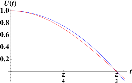
Figure 1: Blue function: $U(t)=-(2t/\pi)^{2}+1$, red function: $U(t)=\cos t$. The two functions are very similar.

C.2 Large initial radius, $U_{0}>U_{c}$

In this case, the dynamics of $U$ is no longer restricted to the region where the potential $V_{\rm pot}(U)$ has linear behavior. Instead the conservation law gives

$$\frac{2U_{0}^{4}}{\lambda}=\frac{N^{2}}{2\lambda}\dot{U}^{2}+\frac{2U^{4}}{\lambda}+cN^{2}U\,.$$ (89)

Again we have oscillatory behavior. Near the turning point

$$\frac{U_{0}^{4}}{\lambda}>N^{2}U_{0}$$ (90)

so the amplitude is very well approximated by $U_{0}$, $\widetilde{U}_{0}\approx U_{0}$.

During each oscillation $U$ starts from $U_{0}$, passes by $U=U_{c}$ given in Eq. (82), then enters the region where $U<U_{c}$. The timescale for $U$ to run from $U=U_{0}$ to $U=U_{c}$, which we call $\Delta\tau_{1}$, is given by

$$\Delta\tau_{1}=N\int^{U_{0}}_{U_{c}}\frac{dU}{\sqrt{U_{0}^{4}-U^{4}-\lambda N^{2}U}}\sim N\int^{U_{0}}_{U_{c}}\frac{dU}{\sqrt{U_{0}^{4}-U^{4}}}\sim\frac{N}{U_{0}}\,,$$ (91)

since in this region the potential $V_{\rm pot}(U)$ is well approximated by the quartic term. On the other hand, the timescale for $U$ to run from $U=U_{c}$ to $U=0$, which we call $\Delta\tau_{2}$, is

$$\Delta\tau_{2}=N\int^{U_{c}}_{0}\frac{dU}{\sqrt{U_{0}^{4}-U^{4}-\lambda N^{2}U}}\lesssim N\int^{U_{c}}_{0}\frac{dU}{\sqrt{U_{0}^{4}}}=N\frac{U_{c}}{U_{0}^{2}}\,.$$ (92)

since in this region the potential is well approximated by the linear term.

Since $U_{c}<U_{0}$, note that $\Delta\tau_{1}>\Delta\tau_{2}$, and therefore the period of oscillation is dominated by the motion from $U_{0}$ to $U_{c}$. The conservation law is well approximated by neglecting the back reaction from open string creation and taking

$$\frac{2U_{0}^{4}}{\lambda}=\frac{N^{2}}{2\lambda}\dot{U}^{2}+\frac{2U^{4}}{\lambda}\,.$$ (93)

Taking $t=0$ at $U=0$ we find the solution

$$U(t)=U_{0}\,\text{sn}\left(\frac{2U_{0}t}{N},-1\right)$$ (94)

where $\text{sn}(u,m)$ is a Jacobi elliptic function, given by

$$\text{sn}(u,m)=\sin\phi\quad\mbox{where $\phi$ is defined by}\quad u=\int_{0}^{\phi}\frac{ds}{\sqrt{1-m\sin^{2}s}}\,\,.$$ (95)

In our case $m=-1$ so $u=\int_{0}^{\phi}\frac{ds}{\sqrt{1+\sin^{2}s}}$. Since $\text{sn}(u,m)=\sin\phi$ is periodic under $\phi\sim\phi+2\pi$, it follows that $u$ is periodic under $u\sim u+\int_{0}^{2\pi}\frac{ds}{\sqrt{1+\sin^{2}s}}\approx u+2\pi/1.2$. In fact, the behavior of $U(t)$ is very well approximated by

$$U(t)=U_{0}\,\text{sn}\left(\frac{2U_{0}t}{N},-1\right)\approx U_{0}\sin{\frac{2.4U_{0}t}{N}}\,.$$ (96)

Figure 2 shows that this approximation works very well. This means $U(t)$ can be approximated as

$$U(t)\approx\widetilde{U}_{0}\sin\Omega t\,,\quad\widetilde{U}_{0}\sim U_{0}\,,\quad\Omega\sim\tau^{-1}\sim\frac{U_{0}}{N}\,.$$ (97)

Note that (88) and (97) agree at $U_{0}\sim U_{c}$.

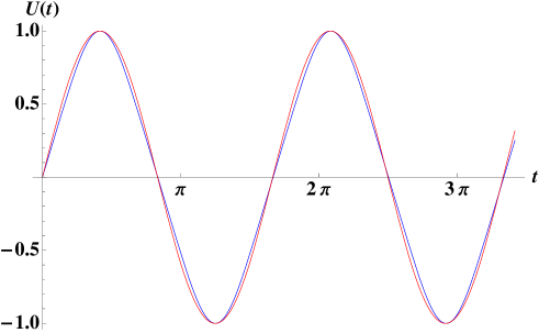
Figure 2: Blue function: $U(t)=\text{sn}(t,-1)$, red function: $U(t)=\sin(1.2t)$. The two functions are very similar.

References

- [1] N. Iizuka, D. Kabat, S. Roy, and D. Sarkar, “Black hole formation at the correspondence point,” arXiv:1303.7278 [hep-th].
- [2] N. Itzhaki, J. M. Maldacena, J. Sonnenschein, and S. Yankielowicz, “Supergravity and the large N limit of theories with sixteen supercharges,” Phys.Rev. D58 (1998) 046004, arXiv:hep-th/9802042 [hep-th].
- [3] G. T. Horowitz and J. Polchinski, “A correspondence principle for black holes and strings,” Phys.Rev. D55 (1997) 6189–6197, arXiv:hep-th/9612146 [hep-th].
- [4] H. Steinacker, “Non-commutative geometry and matrix models,” PoS QGQGS2011 (2011) 004, arXiv:1109.5521 [hep-th].
- [5] D. Berenstein and D. Trancanelli, “Dynamical tachyons on fuzzy spheres,” Phys.Rev. D83 (2011) 106001, arXiv:1011.2749 [hep-th].
- [6] C. Asplund, D. Berenstein, and D. Trancanelli, “Evidence for fast thermalization in the plane-wave matrix model,” Phys.Rev.Lett. 107 (2011) 171602, arXiv:1104.5469 [hep-th].
- [7] P. Riggins and V. Sahakian, “On black hole thermalization, D0 brane dynamics, and emergent spacetime,” Phys.Rev. D86 (2012) 046005, arXiv:1205.3847 [hep-th].
- [8] C. T. Asplund, D. Berenstein, and E. Dzienkowski, “Large N classical dynamics of holographic matrix models,” arXiv:1211.3425 [hep-th].
- [9] J. J. Sakurai and J. Napolitano, Modern quantum mechanics. Addison-Wesley, 2011. See section 3.11.
- [10] J. Madore, “The fuzzy sphere,” Class.Quant.Grav. 9 (1992) 69–88.
- [11] A. Balachandran, S. Kurkcuoglu, and S. Vaidya, “Lectures on fuzzy and fuzzy SUSY physics,” arXiv:hep-th/0511114 [hep-th].
- [12] P. Aschieri, T. Grammatikopoulos, H. Steinacker, and G. Zoupanos, “Dynamical generation of fuzzy extra dimensions, dimensional reduction and symmetry breaking,” JHEP 0609 (2006) 026, arXiv:hep-th/0606021 [hep-th]. See appendix 5.1.
- [13] T. Banks, W. Fischler, S. Shenker, and L. Susskind, “M theory as a matrix model: A conjecture,” Phys.Rev. D55 (1997) 5112–5128, arXiv:hep-th/9610043 [hep-th].
- [14] D. N. Kabat and W. Taylor, “Spherical membranes in matrix theory,” Adv.Theor.Math.Phys. 2 (1998) 181–206, arXiv:hep-th/9711078 [hep-th].
- [15] S.-J. Rey, “Gravitating M(atrix) Q balls,” arXiv:hep-th/9711081 [hep-th].
- [16] B. de Wit, J. Hoppe, and H. Nicolai, “On the quantum mechanics of supermembranes,” Nucl.Phys. B305 (1988) 545.
- [17] P. Collins and R. Tucker, “Classical and quantum mechanics of free relativistic membranes,” Nucl.Phys. B112 (1976) 150.
- [18] Harold Steinacker, private communication.
- [19] L. Susskind, “Holography in the flat space limit,” arXiv:hep-th/9901079 [hep-th].
- [20] J. Polchinski, “M theory and the light cone,” Prog.Theor.Phys.Suppl. 134 (1999) 158–170, arXiv:hep-th/9903165 [hep-th].
- [21] G. T. Horowitz and V. E. Hubeny, “Quasinormal modes of AdS black holes and the approach to thermal equilibrium,” Phys.Rev. D62 (2000) 024027, arXiv:hep-th/9909056 [hep-th].
- [22] N. Iizuka, D. N. Kabat, G. Lifschytz, and D. A. Lowe, “Stretched horizons, quasiparticles and quasinormal modes,” Phys.Rev. D68 (2003) 084021, arXiv:hep-th/0306209 [hep-th].
- [23] K. Maeda, M. Natsuume, and T. Okamura, “Quasinormal modes for nonextreme Dp-branes and thermalizations of super-Yang-Mills theories,” Phys.Rev. D72 (2005) 086012, arXiv:hep-th/0509079 [hep-th].
- [24] S. M. Barnett and P. M. Radmore, Methods in theoretical quantum optics. Oxford Univ. Press, 1997.