A spatiospectral localization approach to estimating potential fields on the surface of a sphere from noisy, incomplete data
taken at satellite altitudes

Abstract

Satellites mapping the spatial variations of the gravitational or magnetic fields of the Earth or other planets ideally fly on polar orbits, uniformly covering the entire globe. Thus, potential fields on the sphere are usually expressed in spherical harmonics, basis functions with global support. For various reasons, however, inclined orbits are favorable. These leave a “polar gap”: an antipodal pair of axisymmetric polar caps without any data coverage, typically smaller than 10^∘ in diameter for terrestrial gravitational problems, but 20^∘ or more in some planetary magnetic configurations. The estimation of spherical harmonic field coefficients from an incompletely sampled sphere is prone to error, since the spherical harmonics are not orthogonal over the partial domain of the cut sphere. Although approaches based on wavelets have gained in popularity in the last decade, we present a method for localized spherical analysis that is firmly rooted in spherical harmonics. We construct a basis of bandlimited spherical functions that have the majority of their energy concentrated in a subdomain of the unit sphere by solving Slepian’s (1960) concentration problem in spherical geometry, and use them for the geodetic problem at hand. Most of this work has been published by us elsewhere. Here, we highlight the connection of the “spherical Slepian basis” to wavelets by showing their asymptotic self-similarity, and focus on the computational considerations of calculating concentrated basis functions on irregularly shaped domains.

1 INTRODUCTION

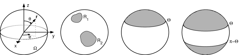
Figure 1: Geometry of the geodetic estimation problem: a concentration region of arbitrary geometry; an axisymmetric polar cap, shaded, of colatitudinal radius $\Theta$; an antipodal pair of polar caps, shaded, representing the geodetic polar gap.

Constructing local spherical harmonic bases that are orthogonal over limited domains and still behave well under the action of up- and downward continuation operators is of interest in geomagnetism [2, 3] and geodesy [4, 5]. As an alternative to a wavelet basis [6, 7], we construct a new basis of so-called Slepian functions [8] on the sphere. These bandlimited functions are designed to have the majority of their energy optimally concentrated inside the geographically limited region covered by satellites, as in Fig. 1. Slepian functions are orthogonal on both the entire as well as the cut sphere, a property that can be exploited to our advantage. Elsewhere [5] we have studied the inverse problem of retrieving a potential field on the unit sphere from noisy and incomplete but continuously available observations made at an altitude above their source. We have obtained exact expressions for the estimation error due to the traditional method of damped least-squares spherical harmonic analysis as well as that arising from a new approach which uses a truncated set of Slepian basis functions.

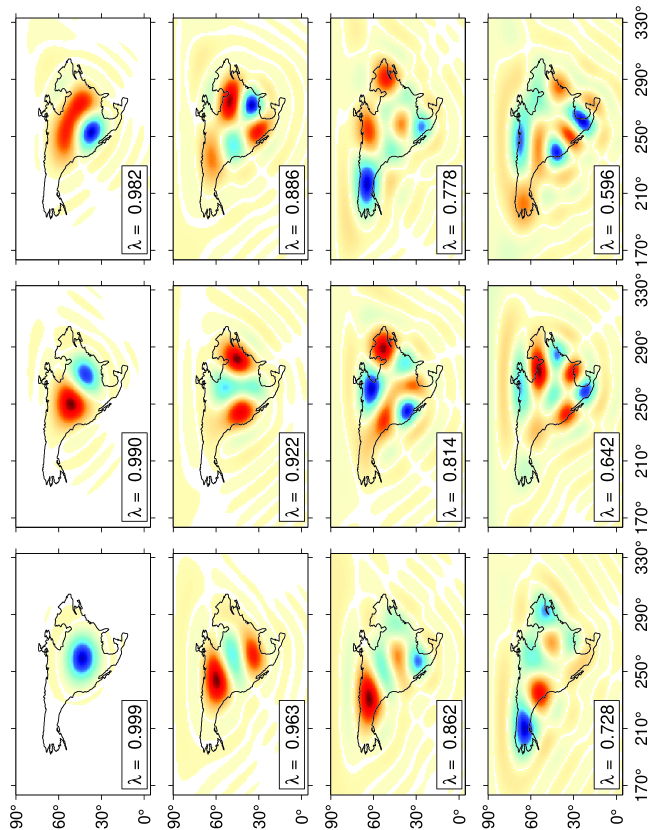
Figure 2: Bandlimited $L=18$ eigenfunctions $g_{1},g_{2},\ldots,g_{12}$ that are optimally concentrated within the continent of North America. The concentration factors $\lambda_{1},\lambda_{2},\ldots,\lambda_{12}$ are indicated; the Shannon number is $N=14$.

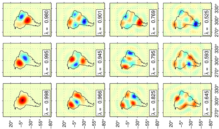
Figure 3: Bandlimited $L=18$ eigenfunctions $g_{1},g_{2},\ldots,g_{12}$ that are optimally concentrated within the continent of South America. The Shannon number is $N=13$. Format is identical to that in Fig. 2.

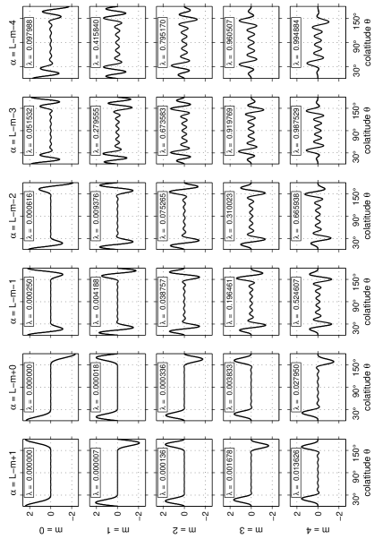
Figure 4: Colatitudinal dependence of the last six fixed-order, $m=0\rightarrow 4$, eigenfunctions $g_{\alpha}(\theta)$, $\alpha=L-m+1\rightarrow L-m-4$, bandlimited to $L=18$. These are generally poorly concentrated in the latitudinal belt $\pm 60^{\circ}$ about the equator, except where the rank $\alpha$ exceeds the fixed-order Shannon number $N_{m}$ (examples in lower right). The functions that have the least energy inside of the equatorial belt, as shown by their low eigenvalues $\lambda_{\alpha}$, are best concentrated inside the complementary polar caps of colatitudinal radius $\Theta=30^{\circ}$.

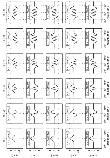
Figure 5: Colatitudinal dependence of the first six fixed-order, $m=0\rightarrow 4$, eigenfunctions $g_{\alpha}(\theta)$, $\alpha=1\rightarrow 6$, bandlimited to $L=18$, that are well concentrated in the latitudinal belt extending $\pm 60^{\circ}$ on either side of the equator. The quality of the spatial concentration is expressed by the labeled eigenvalues $\lambda_{\alpha}$. None of the plotted functions show appreciable energy inside the complementary pair of antipodal polar caps of radius $\Theta=30^{\circ}$.

The geodetic estimation problem can be cast in the much wider context of spatiospectral localization, whereby bandlimited functions are spatially concentrated to regions of arbitrary shape on the sphere [9, 10]. Some of these are illustrated in Figs 2–3. A semi-analytical numerical method can be used to calculate the spherical Slepian functions on a latitudinal belt symmetric about the equator, or its complement, the double polar cap. This approach requires no numerical integration and avoids the construction of matrices other than a tridiagonal matrix whose elements are prescribed analytically. Finding spherical harmonic expressions for bandlimited functions concentrated to polar caps, as in Fig. 4, or latitudinal belts, as in Fig. 5, thus becomes so effortless as to be achievable by a handful of lines of computer code, and the problems with numerical stability that are known to plague alternative approaches [4, 11] are avoided altogether. The key to this “magic” lay hidden in two little-known studies published several decades ago: the work by Gilbert [12] on doubly orthogonal polynomials, and that on commuting differential operators by Grünbaum [13]. It must be remembered that one of Slepian’s main discoveries [8] was the existence of a second-order differential operator that commutes with the spatiospectral localization kernel concentrating to intervals on the real line. Finding the “prolate spheroidal functions” amounts to the diagonalization of a simple tridiagonal matrix [14]. Gilbert [12] presented two additional commuting differential operators, which are applicable to the concentration of Legendre polynomials to one-and two-sided domains. Grünbaum [13] proved that the matrix accompanying the localization to the single polar cap is, once again, tridiagonal, and the same holds for the double polar cap, or its complement, the latitudinal belt, as we have shown [5].

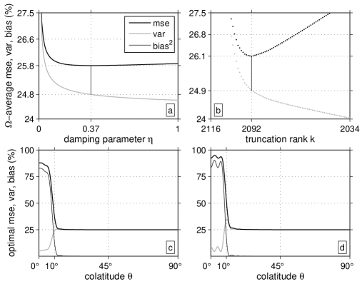
Figure 6: Mean-squared error (mse), variance and bias for the damped least-squares solution to the geodetic inverse problem of recovering the source signal from incomplete and noisy observations, and the truncated Slepian approach [5]. The antipodal polar gap has a radius $\Theta=10^{\circ}$; the bandwidth is $L=45$; signal-to-noise ratio $S/N=4$. Panels a & b show the values averaged over the unit sphere; the squared bias is the difference between the mse and variance curves, indicated by the thin black vertical line. Panels c & d show the values at the optimal damping and truncation levels.

In practice, the geodetic and geomagnetic inverse problems are always ill-conditioned, even in the absence of a polar gap, due the peculiarities of orbital data coverage and the distribution of noise sources [15, 16]. In the standard method of damped spherical harmonic inversion, the ill-conditioning is alleviated by the addition of a small damping parameter to the normal equation matrix prior to inversion. Often the value of this parameter is ad hoc and chosen primarily for numerical stability, but more sophisticated methods use a priori statistical information about the set of model parameters. We have derived the exact structure of the model parameter sensitivity matrix arising from the presence of a contiguous data gap, assuming the data are known continuously everywhere but inside it. The Slepian functions were revealed to be the very eigenfunctions of this matrix. Assuming a particular covariance structure for the model parameters and the observational noise, this knowledge allowed us to write analytical expressions for the optimal regularization terms for the damped spherical harmonic method. Such an approach optimally filters out the small eigenvalues, and thus reduces the ill-conditioning of the sensitivity matrix [17]. Our preferred method [5] applies a hard truncation to the singular values of the sensitivity matrix in an approach based directly on the Slepian expansion of the model. We have showed that this is only marginally less successful in minimizing the mean-squared estimation error, as shown in Fig. 6 for the case of white signal and noise, as well as computationally advantageous and more intuitively appealing.

The problems we posed and solved in this context are not limited to geodesy and observations made from a satellite. In geomagnetism, our observation level may be the Earth’s surface, and the source level at or near the core-mantle boundary [18, 19]. In cosmology, the unit sphere constituting the sky is observed from the inside out, and the galactic plane masking spacecraft measurements has the shape of a latitudinal belt [20]. Ground-based astronomical measurements may be confined to a small circular patch of the sky [21, 22]. Finally, in planetary science, knowledge of the estimation statistics of properties observed over mere portions of the planetary surface is important in the absence of groundtruthing observations.

2 Concentration within an arbitrarily shaped region

We seek to determine those bandlimited functions $g(\mathbf{\hat{r}})$ that are optimally concentrated within a spatial region $R$.

2.1 Spherical harmonics

The geometry of the unit sphere $\Omega=\{\mathbf{\hat{r}}:\|\mathbf{\hat{r}}\|=1\}$ is depicted in Fig. 1. We denote the colatitude of a geographical point $\mathbf{\hat{r}}$ by $0\leq\theta\leq\pi$ and the longitude by $0\leq\phi<2\pi$; the geodesic angular distance between two points $\mathbf{\hat{r}}$ and $\mathbf{\hat{r}}^{\prime}$ will be denoted by $\Delta$. We use $R$ to denote a region of $\Omega$, of area $A$, within which we seek to concentrate a bandlimited function of position $\mathbf{\hat{r}}$. We use real surface spherical harmonics defined by [23, 24]

$$Y_{lm}(\mathbf{\hat{r}})=Y_{lm}(\theta,\phi) = \left\{\begin{array}[]{l@{\quad\mbox{if}\hspace{0.6em}}l}\rule[-5.69054pt]{0.0pt}{17.07164pt}\sqrt{2}X_{lm}(\theta)\cos m\phi\hfil\quad\mbox{if}\hskip 6.00006pt&-l\leq m<0\\ \rule[-5.69054pt]{0.0pt}{17.07164pt}X_{l0}(\theta)\hfil\quad\mbox{if}\hskip 6.00006pt&m=0\\ \rule[-5.69054pt]{0.0pt}{17.07164pt}\sqrt{2}X_{lm}(\theta)\sin m\phi\hfil\quad\mbox{if}\hskip 6.00006pt&0<m\leq l,\\ \end{array}\right.$$ (4)

$$X_{lm}(\theta) = (-1)^{m}\left(\frac{2l+1}{4\pi}\right)^{1/2}\left[\frac{(l-m)!}{(l+m)!}\right]^{1/2}\!P_{lm}(\cos\theta),$$ (5)

$$P_{lm}(\mu) = \frac{1}{2^{l}l!}(1-\mu^{2})^{m/2}\left(\frac{d}{d\mu}\right)^{l+m}\!(\mu^{2}-1)^{l}.$$ (6)

The quantity $0\leq l\leq\infty$ is the angular degree of the spherical harmonic, and $-l\leq m\leq l$ is its angular order. The function $P_{lm}(\mu)$ defined in (6) is the associated Legendre function of integer degree $l$ and order $m$. Our choice of the constants in equations (4)–(5) orthonormalizes the harmonics on the unit sphere:

$$\int_{\Omega}Y_{lm}Y_{l^{\prime}m^{\prime}}\,d\Omega=\delta_{ll^{\prime}}\delta_{mm^{\prime}}.$$ (7)

2.2 Spatial concentration of a bandlimited function to an arbitrarily shaped region

To maximize the spatial concentration of a bandlimited function

$$g=\sum\limits_{l=0}^{L}\sum\limits_{m=-l}^{l}g_{lm}Y_{lm},$$ (8)

within a region $R$, we maximize the ratio

$$\lambda=\int_{R}g^{2}\,d\Omega\left/\int_{\Omega}g^{2}\,d\Omega\right..$$ (9)

Elsewhere, we have shown [10] that maximizing equation (9) leads to the eigenvalue equation

$$\sum\limits_{l^{\prime}=0}^{L}\sum\limits_{m^{\prime}=-l^{\prime}}^{l^{\prime}}D_{lm,l^{\prime}m^{\prime}}g_{l^{\prime}m^{\prime}}=\lambda\hskip 0.50003ptg_{lm},\quad\mbox{where}\quad D_{lm,l^{\prime}m^{\prime}}=\int_{R}Y_{lm}Y_{l^{\prime}m^{\prime}}\,d\Omega.$$ (10)

We have also shown [10] that we may rewrite equation (10) as a spatial-domain eigenvalue equation:

$$\int_{R}D(\mathbf{\hat{r}},\mathbf{\hat{r}}^{\prime})\,g(\mathbf{\hat{r}}^{\prime})\,d\Omega^{\prime}=\lambda\hskip 0.50003ptg(\mathbf{\hat{r}}),\quad\mathbf{\hat{r}}\in\Omega,\quad\mbox{where}\quad D(\mathbf{\hat{r}},\mathbf{\hat{r}}^{\prime})=\sum_{l=0}^{L}\left(\frac{2l+1}{4\pi}\right)\!P_{l}(\cos\Delta).$$ (11)

Equation (11) is a homogeneous Fredholm integral equation of the second kind, with a finite-rank, symmetric, separable kernel [25, 26]. The spectral-domain eigenvalue problem (10) for the spherical harmonic expansion coefficients $g_{lm}$ and the spatial-domain eigenvalue problem (11) for the spatial-domain $g(\mathbf{\hat{r}})$ are completely equivalent. The sum of the eigenvalues of equations (10) or (11) is given by

$$\qquad N=\sum_{\alpha=1}^{(L+1)^{2}}\lambda_{\alpha}=\sum_{l=0}^{L}\sum_{m=-l}^{l}D_{lm,lm}=\int_{R}D(\mathbf{\hat{r}},\mathbf{\hat{r}})\,d\Omega=(L+1)^{2}\,\frac{A}{4\pi}.$$ (12)

This is the spherical analogue of the “Shannon number” in Slepian’s one-dimensional concentration problem [1, 8, 14].

2.3 Spatial concentration of a bandlimited function to azimuthally symmetric regions

In the important special case in which the region of concentration is a circularly symmetric cap of colatitudinal radius $\Theta$, centered on the north pole, as shown in Fig. 1, the matrix elements (10) reduce to [10, 5]

$$D_{ll^{\prime}} = 2\pi\,\int_{0}^{\Theta}X_{lm}X_{l^{\prime}m}\sin\theta\,d\theta\quad\mbox{for each order}\quad 0\leq|m|\leq L,$$ (13)

$$= (-1)^{m}\frac{\sqrt{(2l+1)(2l^{\prime}+1)}}{2}\!\!\sum_{n=|l-l^{\prime}|}^{l+l^{\prime}}\left(\!\begin{array}[]{ccc}l&n&l^{\prime}\\ 0&0&0\end{array}\!\right)\left(\!\begin{array}[]{ccc}l&n&l^{\prime}\\ m&0&\!\!-m\end{array}\!\right)\big{[}P_{n-1}(\cos\Theta)-P_{n+1}(\cos\Theta)\big{]},$$ (18)

where the arrays of indices are Wigner 3-$j$ symbols [24, 23, 27]. For a circularly symmetric double cap of common colatitudinal radius $\Theta$, as in Fig. 1, we obtain [5]

$$D_{ll^{\prime}}=2\pi\left[1+(-1)^{l+l^{\prime}}\right]\int_{0}^{\Theta}X_{lm}X_{l^{\prime}m}\sin\theta\,d\theta\quad\mbox{for each order}\quad 0\leq|m|\leq L.$$ (19)

The double-cap spatial eigenfunctions separate into solutions that are even or odd across the equator [10]. Finally, the single-order equivalent of the spatial-domain kernel (11) is given by [10]

$$D(\mu,\mu^{\prime})=\frac{\displaystyle{(L-m+1)!}}{\displaystyle{2(L+m)!}}\left[\frac{\displaystyle{P_{L+1\,m}(\mu)P_{Lm}(\mu^{\prime})-P_{Lm}(\mu)P_{L+1\,m}(\mu^{\prime})}}{\displaystyle{\mu-\mu^{\prime}}}\right],$$ (20)

where $\mu=\cos(\theta)$ and which can be computed using L’Hôpital’s rule when $\mu=\mu^{\prime}$. For each of the fixed-order eigenvalue problems the partial Shannon number can be computed from

$$N_{m}=\sum_{\alpha=1}^{L-m+1}\!\!\lambda_{\alpha}=\sum\limits_{l=m}^{L}D_{ll}=\int_{\cos\Theta}^{1}D(\mu,\mu)\,d\mu=\frac{\displaystyle{(L-m+1)!}}{\displaystyle{2(L+m)!}}\int_{\cos\Theta}^{1}\big{[}P_{L+1\,m}^{\prime}P_{Lm}-P_{Lm}^{\prime}P_{L+1\,m}\big{]}\,d\mu,$$ (21)

where the prime denotes differentiation with respect to $\mu$. Once the $L+1$ sequences of fixed-order eigenvalues have been found, they can be resorted to exhibit an overall mixed-order ranking. The total number of significant eigenvalues (12) is then

$$N=N_{0}+2\sum_{m=1}^{L}N_{m},$$ (22)

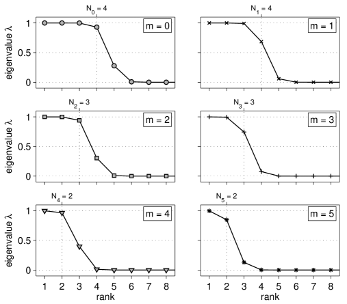
Figure 7: Fixed-order eigenvalue spectra for an axisymmetric polar cap of radius $\Theta=40^{\circ}$. The maximal spherical harmonic degree is $L=18$. A different symbol is used to plot $\lambda_{\alpha}$ versus rank $\alpha$ for each order $0\leq m\leq 5$. The total number of fixed-order eigenvalues is $L-m+1$; only the largest eight ($\lambda_{1}$ through $\lambda_{8}$) are shown. Vertical grid lines and top labels specify the partial Shannon numbers $N_{m}$, rounded to the nearest integer.

where the factor of two accounts for the $\pm m$ degeneracy. Fig. 7 shows the fixed-order eigenvalue spectra for $0\leq m\leq 5$. The cap radius is $\Theta=40^{\circ}$ and the maximal spherical harmonic degree is $L=18$. The partial Shannon numbers $N_{m}$, computed by rounding equation (21) to the nearest integer, are shown. As in the case of the classical Slepian problem [28, 14, 29] the spectra have a characteristic step shape, showing significant ($\lambda\approx 1$) and insignificant ($\lambda\approx 0$) eigenvalues separated by a narrow transition band. The partial Shannon number (21) provides a good estimate of the number of well concentrated eigenfunctions; the first $N_{m}$ eigenfunctions all have a concentration factor exceeding $\lambda=0.5$.

As we showed elsewhere [10, 5], equation (10) for the single cap is equivalent to an algebraic eigenvalue equation that requires diagonalization of a matrix that commutes with (13)–(18) and whose elements are given by

$$T_{ll} = -l(l+1)\cos{\Theta},$$

$$T_{l\,l+1} = \big{[}l(l+2)-L(L+2)\big{]}\sqrt{\frac{\displaystyle{(l+1)^{2}-m^{2}}}{\displaystyle{(2l+1)(2l+3)}}},$$ (23)

and we can replace the matrix (19) for functions odd ($p=o$) or even ($p=e$) across the equator by the matrix

$$T^{p}_{ll} = -l(l+1)\cos^{2}{\Theta}+\frac{2}{2l+3}\left[(l+1)^{2}-m^{2}\right]+[(l-2)(l+1)-L_{p}(L_{p}+3)]\left[\frac{1}{3}-\frac{2}{3}\,\frac{\displaystyle{3m^{2}-l(l+1)}}{\displaystyle{(2l+3)(2l-1)}}\right],$$

$$T^{p}_{l\,l+2} = \frac{\displaystyle{\big{[}l(l+3)-L_{p}(L_{p}+3)\big{]}}}{\displaystyle{2l+3}}\sqrt{\frac{\displaystyle{\left[(l+2)^{2}-m^{2}\right]\left[(l+1)^{2}-m^{2}\right]}}{\displaystyle{(2l+5)(2l+1)}}}.$$ (24)

for the double cap, where $L_{e}$ and $L_{o}$ are $L$ and $L-1$, respectively, if $m$ and $L$ have the same parity, and $L-1$ and $L$, respectively, if $m$ and $L$ have opposite parity. Thus, equation (24) defines two matrices, one for the even and one for the odd functions; both are properly speaking tridiagonal [5].

3 Asymptotic scaling

The eigenvalues $\lambda_{1},\lambda_{2},\ldots$ and suitably scaled eigenfunctions $\psi_{1}(x),\psi(x)_{2},\ldots$ of Slepian’s time series problem [1], of optimally concentrating a strictly bandlimited signal with a spectrum that vanishes for frequencies $|\omega|>W$ into a time interval $|t|\leq T$, in other words, the eigenvalues and eigenfunctions of

$$\int_{-1}^{1}\frac{\displaystyle{\sin TW(x-x^{\prime})}}{\displaystyle{\pi(x-x^{\prime})}}\,\psi(x^{\prime})\,dx^{\prime}=\lambda\hskip 0.50003pt\psi(x),\quad|x|\leq 1,$$ (25)

depend only upon the “Shannon number” $N=2TW/\pi$. This scaling is the only important feature of the one-dimensional problem that does not carry over to the spatiospectral concentration problem on a sphere. Shannon-number scaling on a sphere is exhibited only asymptotically, in the limit

$$A\rightarrow 0,\quad L\rightarrow\infty,\quad\mbox{with}\quad N=(L+1)^{2}\frac{\displaystyle{A}}{\displaystyle{4\pi}}\quad\mbox{held fixed}.$$ (26)

In that limit of a small concentration area $A$ and a large bandwidth $0\leq l\leq L$, the curvature of the sphere becomes negligible and the spherical concentration problem approaches the concentration problem in the plane [30].

3.1 Scaled integral equation for an arbitrarily shaped region

Two results underlie the consideration of the flat-Earth limit (26), which we undertake in this section. The first is Hilb’s asymptotic approximation for the Legendre functions [31, 32, 33, 34],

$$X_{lm}(\theta)\approx(-1)^{m}\sqrt{\frac{l+1/2}{2\pi}}\,\sqrt{\frac{\theta}{\sin\theta}}\,J_{m}\big{[}(l+1/2)\theta\big{]},\quad 0\leq\theta\ll\pi,$$ (27)

where $J_{m}(x)$ is the Bessel function of the first kind; the second is the truncated Watson-Poisson sum formula [23],

$$\sum\limits_{l=0}^{L}{f}(l+1/2)=\sum_{s=-\infty}^{\infty}(-1)^{s}\int_{0}^{L+1}{f}(k)e^{-2\pi isk}\,dk,$$ (28)

valid for an arbitrary continuous function $f(x)$. An application of (27) and (28), substituting $k=(L+1)p$ and taking the limit $L\rightarrow\infty,\Delta\rightarrow 0$, with the product $L\Delta$ held fixed, enables us to write the Fredholm kernel $D(\mathbf{\hat{r}},\mathbf{\hat{r}}^{\prime})$ of equation (11) in the form

$$D(\Delta)\approx\frac{(L+1)^{2}}{2\pi}\int_{0}^{1}J_{0}\big{[}(L+1)p\Delta\big{]}\,p\,dp=\frac{(L+1)\,J_{1}\big{[}(L+1)\Delta\big{]}}{2\pi\Delta},$$

where we have made the approximation $\Delta/\!\sin\Delta\approx 1$, and used the Riemann-Lebesgue lemma [35] to eliminate the $s\not=0$ terms involving the highly oscillatory factors $e^{-2\pi is(L+1)p}$. In the limit $x\rightarrow 0$ the ratio $J_{1}(x)/x\rightarrow 1/2$, so the $\Delta\rightarrow 0$ limit of (3.1) is $D(0)=(L+1)^{2}/(4\pi)$, guaranteeing that the Shannon number remains unchanged.

To obtain a scaled version of equation (11) dependent only upon the Shannon number $N$, we make use of the approximation (3.1) for the kernel $D(\mathbf{\hat{r}},\mathbf{\hat{r}}^{\prime})$, and introduce the independent and dependent variable transformations

$${\bf x}=\sqrt{\frac{\displaystyle{4\pi}}{\displaystyle{A}}}\,\mathbf{\hat{r}},\quad{\bf x}^{\prime}=\sqrt{\frac{\displaystyle{4\pi}}{\displaystyle{A}}}\,\mathbf{\hat{r}}^{\prime},\qquad\psi({\bf x})=g(\mathbf{\hat{r}}),\quad\psi({\bf x}^{\prime})=g(\mathbf{\hat{r}}^{\prime}).$$ (29)

The scaled coordinates ${\bf x},{\bf x}^{\prime}$ are the projections of the points $\mathbf{\hat{r}},\mathbf{\hat{r}}^{\prime}\in\Omega$ onto a large sphere $\Omega_{*}$ of squared radius $\|{\bf x}\|^{2}=4\pi/A$. The geodesic distance between the points ${\bf x},{\bf x}^{\prime}\in\Omega_{*}$ and the differential surface area on $\Omega_{*}$ are

$$\|{\bf x}-{\bf x}^{\prime}\|=\sqrt{\frac{\displaystyle{4\pi}}{\displaystyle{A}}}\,\Delta\quad\mbox{and}\quad d\Omega_{*}=\frac{4\pi}{A}\,d\Omega.$$ (30)

Upon making the substitutions (29)–(30), equations (11) and (3.1) reduce to

$$\int_{R_{*}}\!\!D_{*}({\bf x},{\bf x}^{\prime})\,\psi({\bf x^{\prime}})\,d\Omega_{*}^{\prime}=\lambda\hskip 1.00006pt\psi({\bf x}),\quad\mbox{with}\quad D_{*}({\bf x},{\bf x}^{\prime})=\frac{\displaystyle{\sqrt{N}}}{\displaystyle{2\pi}}\,\frac{\displaystyle{J_{1}\big{(}\raisebox{-0.86108pt}{$\sqrt{N}$}\,\|{\bf x}-{\bf x}^{\prime}\|\big{)}}}{\displaystyle{\|{\bf x}-{\bf x}^{\prime}\|}},$$ (31)

where $R_{*}$, of area $4\pi$, is the projection of the region of concentration $R$ onto the sphere $\Omega_{*}$ and $D_{*}({\bf x},{\bf x}^{\prime})$ is the symmetric, $N$-dependent Fredholm kernel. Equation (31) is the spherical analogue of the one-dimensional scaled eigenvalue equation (25). The asymptotic eigenvalues $\lambda_{1},\lambda_{2},\ldots$ and associated scaled eigenfunctions $\psi_{1}({\bf x}),\psi_{2}({\bf x}),\ldots$ depend upon the maximal degree $L$ and the area $A$ only through the Shannon number. As in the case of equation (11), we are free to solve (31) either on all of $\Omega_{*}$, in which case the eigenfunctions $\psi_{1}({\bf x}),\psi_{2}({\bf x}),\ldots$ are bandlimited, or only in the region of concentration $R_{*}$, in which case they are spacelimited. It is readily verified that the scaling has no effect upon the sum of the eigenvalues.

In the limit (26), we expect the exact Fredholm kernel (11), evaluated on $\Omega_{*}$ and normalized by its value at zero offset,

$$\frac{\displaystyle{D\big{(}\sqrt{4\pi/A}\,\Delta\big{)}}}{\displaystyle{D(0)}}=\frac{1}{(L+1)^{2}}\sum\limits_{l=0}^{L}(2l+1)\,P_{l}\!\left(\cos\sqrt{\frac{4\pi}{A}}\,\Delta\right),$$ (32)

to be well approximated by the similarly normalized asymptotic kernel

$$\frac{\displaystyle{D_{*}(\Delta)}}{\displaystyle{D_{*}(0)}}=\frac{2J_{1}(\sqrt{N}\Delta)}{\sqrt{N}\Delta}.$$ (33)

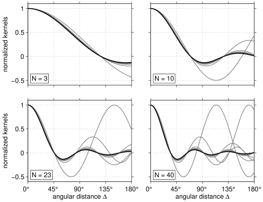
Figure 8: Comparison of the exact scaled kernels (32) with the flat-Earth asymptotic approximation (33) (black). The Shannon number $N=3,10,23,40$ is kept constant in each of the four panels, and the bandwidth used to compute the exact scaled kernels varies between $L=1$ (worst fitting) and $L=100$ (best fitting).

The quality of this asymptotic approximation to the kernel and the associated flat-Earth scaling are illustrated in Fig. 8. In the four examples shown, with Shannon numbers $N=3,10,23,40$, the approximation is excellent even for angular distances as large as $\Delta\approx 135^{\circ}$, once the maximal spherical harmonic degree exceeds $L=3$ – $4$.

3.2 Asymptotic fixed-order Shannon number

The asymptotic approximation to the number of significant eigenvalues associated with a given order $m$ is

$$N_{m} = \int_{0}^{1}D_{*}(x,x)\,x\,dx=4N\int_{0}^{1}\!\!\int_{0}^{1}\!J_{m}^{2}\big{(}2\sqrt{N}\,p\hskip 1.00006ptx\big{)}\,p\,dp\,x\,dx$$ (34)

$$= N^{m+1}{}_{2}F_{3}(1+m,1/2+m;1+2m,2+m,2+m;-4N)/\left[\Gamma(2+m)\right]^{2}$$

$$= 2N\left[J^{2}_{m}(2\sqrt{N})+J^{2}_{m+1}(2\sqrt{N})\right]-(2m+1)\sqrt{N}J_{m}(2\sqrt{N})J_{m+1}(2\sqrt{N})$$

$${}-\frac{m}{2}\Big{[}1-J_{0}^{2}(2\sqrt{N})-2\sum\limits_{n=1}^{m}J_{n}^{2}(2\sqrt{N})\Big{]},$$

where $F$ is a generalized hypergeometric function and $\Gamma$ the gamma function. The relationship (22) between the total number $N$ of significant eigenvalues and the number $N_{m}$ associated with each order $m$ is preserved in this asymptotic approximation, inasmuch as, by virtue of the identity $J_{0}^{2}(x)+2\sum_{m=1}^{\infty}J_{m}^{2}(x)=1$,

$$N=4N\int_{0}^{1}\!\!\int_{0}^{1}\left[J_{0}^{2}\big{(}2\sqrt{N}pq\big{)}+2\sum\limits_{m=1}^{\infty}J^{2}_{m}\big{(}2\sqrt{N}pq\big{)}\right]\,p\,dp\,x\,dx=4N\int_{0}^{1}\!\!\int_{0}^{1}\,p\,dp\,x\,dx=N.$$ (35)

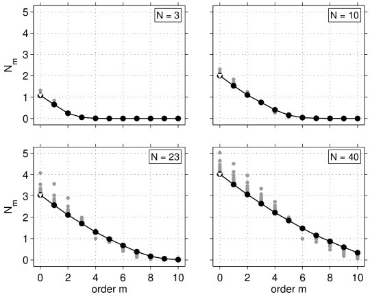
Figure 9: Comparison of the number $N_{m}$ of significant eigenvalues of fixed order $m$ (gray) with the asymptotic approximation (34) (black). The Shannon number $N=3,10,23,40$ is kept constant in each of the four panels, and the bandwidth used to compute the exact values of $N_{m}$ varies between $L=1$ (worst fitting) and $L=100$ (best fitting). Points inconsistent with the constraint $A/(4\pi)=N/(L+1)^{2}<1$ are not plotted. White triangles show the simplified zonal ($m=0$) approximation $N_{0}\approx(L+1)\Theta/\pi$.

In Fig. 9 we compare the exact fixed-order Shannon numbers $N_{m}$, computed by Gauss-Legendre numerical integration of equation (21), with the asymptotic result (34), for the same values of $N=3,10,23,40$ and $1\leq L\leq 100$ as in Fig. 8. The number of significant $m=0$ eigenvalues can be even more simply approximated by $N_{0}\approx 2\sqrt{N}/\pi\approx(L+1)\Theta/\pi$, as shown. This can be derived using the large-argument asymptotic expansion of the Bessel function [36, 35]. The result (34) is exact in the case of concentration in a two-dimensional plane.

4 Computational considerations

All of the computations described here have been performed using double precision arithmetic. Statements regarding machine precision refer to double precision, with a round-off error of $\sim\!10^{-16}$.

4.1 Concentration within a polar cap

We may compute the colatitudinal eigenfunctions $g_{1}(\theta),g_{2}(\theta),\ldots,g_{L-m+1}(\theta)$ of an axisymmetric polar cap with $0\leq\theta\leq\Theta$ using three different methods. The first is by numerical diagonalization of the $(L-m+1)\times(L-m+1)$ matrix in equations (13)–(18). We may either implement the Wigner 3-$j$ expression (18) for the elements $D_{ll^{\prime}}$, or use Gauss-Legendre quadrature [37] to evaluate the defining integral (13):

$$D_{ll^{\prime}}=\int_{\cos\Theta}^{1}X_{lm}(\arccos\mu)X_{l^{\prime}m}(\arccos\mu)\,d\mu\approx\sum_{j=1}^{J}w_{j}X_{lm}(\arccos\mu_{j})X_{l^{\prime}m}(\arccos\mu_{j}),$$ (36)

where $\mu_{1},\mu_{2},\ldots,\mu_{J}$ are roots of the Legendre polynomial $P_{J}(\bar{\mu})$, rescaled from $-1\leq\bar{\mu}_{j}\leq 1$ to $\cos\Theta\leq\mu_{j}\leq 1$, and $w_{j}=2(1-\bar{\mu}_{j}^{2})^{-1}[P_{J}^{\prime}(\bar{\mu}_{j})]^{-2}$, with $j=1,2,\ldots,J$ are the associated integration weights. Only the uppermost triangular matrix elements $D_{ll^{\prime}},l\leq l^{\prime}$ are computed explicitly; the lowermost elements are infilled using the symmetry $D_{ll^{\prime}}=D_{l^{\prime}l}$. The order of the Gauss-Legendre integration is adjusted upward until the $L-m+1$ spatial-domain eigenfunctions $g_{1}(\theta),g_{2}(\theta),\ldots,g_{L-m+1}(\theta)$ satisfy the orthogonality relations

$$2\pi\int_{0}^{\pi}g_{\alpha}g_{\beta}\sin\theta\,d\theta=\delta_{\alpha\beta}\quad\mbox{and}\quad 2\pi\int_{0}^{\Theta}g_{\alpha}g_{\beta}\sin\theta\,d\theta=\lambda_{\alpha}\delta_{\alpha\beta}.$$ (37)

to within machine precision. The same high-order Gauss-Legendre quadrature rule is used to evaluate the orthogonality integrals. The Legendre functions $X_{lm}(\theta)$ are computed with high accuracy to very high degree ($l\approx 500$) using a recursive algorithm [38, 39].

The second method is by solving the fixed-order version of the Fredholm equation (11) via the Nystrom method [37]. Discretizing this equation by Gauss-Legendre quadrature we obtain

$$\sum_{j^{\prime}=1}^{J}w_{j^{\prime}}D(\mu_{j},\mu^{\prime}_{j^{\prime}})g(\mu^{\prime}_{j^{\prime}})=\lambda\hskip 0.50003ptg(\mu_{j}),\quad j=1,2,\ldots,J.$$ (38)

Equation (38) can be rewritten as a symmetric algebraic eigenvalue equation,

$$({\textsf{\small W}}\tilde{{\textsf{D}}}{\textsf{\small W}})({\textsf{\small W}}\tilde{\textsf{g}})=\lambda\hskip 0.50003pt({\textsf{\small W}}\tilde{\textsf{g}}),$$ (39)

where $\tilde{\textsf{g}}$ is a $J$-dimensional column vector with entries $\tilde{g}_{j}=g(\mu_{j})$, and where $\tilde{{\textsf{D}}}$ and W denote the $J\times J$ matrices with elements $\tilde{D}_{jj^{\prime}}=D(\mu_{j},\mu^{\prime}_{j^{\prime}})$ and $W_{jj^{\prime}}=\sqrt{w_{j}}\,\delta_{jj^{\prime}}$. The eigenvalues $\lambda$ and transformed eigenvectors ${\textsf{\small W}}\tilde{\textsf{g}}$ are computed by numerical diagonalization of the matrix ${\textsf{\small W}}\tilde{{\textsf{D}}}{\textsf{\small W}}$. The order of integration $J$ is again chosen to ensure accurate orthogonality of the spatial-domain eigenfunctions $g_{1}(\theta),g_{2}(\theta),\ldots,g_{L-m+1}(\theta)$. In the zonal ($m=0$) case the choice $J=L+1$ renders both of the integrations (36) and (38) exact; for $m\not=0$ we use a conservative, larger integration order $J$, since the integrands are no longer polynomials.

Even for moderate values of the bandwidth $L$ and cap radius $\Theta$, the smallest eigenvalues $\ldots,\lambda_{L-m},\lambda_{L-m+1}$ fall below machine precision. The associated, least well concentrated eigenfunctions computed using either of the above two direct methods are in that case essentially arbitrary orthogonal members of a numerically degenerate eigenspace, and are no longer accurate [4]. Because of this, it is not possible to find the optimally excluded eigenfunctions of a small polar cap, or equivalently the optimally concentrated eigenfunctions of a large cap, by matrix diagonalization of (36). Fortunately, this difficulty can be overcome by the third method, which is numerical diagonalization of the tridiagonal Grünbaum matrix (23). The roughly equant spacing of their eigenvalues enables all of the associated eigenfunctions to be calculated to within machine precision. The spatiospectral concentration factors $\lambda_{1},\lambda_{2},\ldots,\lambda_{L-m+1}$ are computed to the same precision, either by a posteriori matrix multiplication via (10), or by Gauss-Legendre integration of the orthogonality relation (37). Both the significant and the insignificant eigenvalues computed using each of the above methods agree to within machine precision, providing a useful numerical check. Diagonalization of the tridiagonal matrix (23) is the only numerically stable way to solve the concentration problem for either a large polar cap or a large bandwidth $L$. By extension, it is even possible to use this formalism to compute spacelimited eigenfunctions that are in the null space [41]. The above results apply to the double-cap case if using the appropriate Grünbaum matrix (24).

4.2 Concentration within an arbitrarily shaped region

We solve the spatiospectral concentration problem for an arbitrarily shaped region $R$ by numerical diagonalization of the $(L+1)^{2}\times(L+1)^{2}$ matrix with elements $D_{lm,l^{\prime}m^{\prime}}$ defined by equation (10). Given a (splined) boundary of $R$, we first find the northernmost and southernmost points, with colatitudes $\theta_{\rm n}$ and $\theta_{\rm s}$. For every $\theta_{\rm n}\leq\theta\leq\theta_{\rm s}$, we then find the easternmost and westernmost points, with longitudes $\phi_{\rm e}(\theta)$ and $\phi_{\rm w}(\theta)$. In the case of a non-convex region with indentations and protuberances, there may be several such eastern and western boundary points, which we shall index with an additional subscript $i=1,2,\ldots,I$. The integral over longitude,

$$\Phi_{mm^{\prime}}(\theta)=\sum_{i=1}^{I}\int_{\phi_{{\rm w}i}}^{\phi_{{\rm e}i}}\!\left\{\!\!\begin{array}[]{c}\cos m\phi\\ \sin m\phi\end{array}\!\!\right\}\left\{\!\!\begin{array}[]{c}\cos m^{\prime}\phi\\ \sin m^{\prime}\phi\end{array}\!\!\right\}d\phi,$$ (40)

is done analytically, and we use Gauss-Legendre quadrature to compute the remaining integral over colatitude:

$$D_{lm,l^{\prime}m^{\prime}} = \int_{\mu_{\rm n}}^{\mu_{\rm s}}X_{lm}(\arccos\mu)X_{l^{\prime}m^{\prime}}(\arccos\mu)\Phi_{mm^{\prime}}(\arccos\mu)\,d\mu$$ (41)

$$\approx \sum_{j=1}^{J}w_{j}X_{lm}(\arccos\mu_{j})X_{l^{\prime}m^{\prime}}(\arccos\mu_{j})\Phi_{mm^{\prime}}(\arccos\mu_{j}).$$

As in the case of a polar cap, we adjust the order of the integration $J$ upward until the spatial-domain eigenfunctions $g_{1}(\mathbf{\hat{r}}),g_{2}(\mathbf{\hat{r}}),\ldots,g_{(L+1)^{2}}(\mathbf{\hat{r}})$ satisfy the orthogonality relations

$$\int_{\Omega}g_{\alpha}g_{\beta}\,d\Omega=\delta_{\alpha\beta},\quad\mbox{and}\quad\int_{R}g_{\alpha}g_{\beta}\,d\Omega=\lambda_{\alpha}\delta_{\alpha\beta}.$$ (42)

to within machine precision. There is no analogue to Grünbaum’s procedure for an arbitrarily shaped region, so only the eigenfunctions associated with eigenvalues that are above machine precision can be computed accurately. In most practical applications[5], this is not a limitation, since we are generally interested only in the computable, well concentrated eigenfunctions $g_{1}(\mathbf{\hat{r}}),g_{2}(\mathbf{\hat{r}}),\ldots,g_{N}(\mathbf{\hat{r}})$, which are associated with the numerically significant eigenvalues $\lambda_{1},\lambda_{2},\ldots,\lambda_{N}$ where $N$ is the Shannon number (12).

4.3 Concentration within a non-polar circular cap

One of the principal applications of spherical Slepian functions in geophysics and planetary physics[42, 43, 44, 45] is to analyze measurements within a circularly symmetric region centered upon an arbitrary geographical location $\theta_{0},\phi_{0}$. The preferred procedure for determining the required optimally concentrated eigenfunctions is first to compute the spherical harmonic coefficients $g_{lm}$ of the eigenfunctions concentrated within a polar cap $0\leq\theta\leq\Theta$, and then to rotate these to the desired cap location [46, 23, 24, 39]. The actual windowing of the data for further analysis may either be carried out in the spectral domain [45], or, more simply, by straightforward multiplication after transformation of the rotated eigenfunctions to the spatial domain. If one wishes to avoid spherical harmonic rotation, it is also possible to compute the rotated eigenfunctions directly, by performing the numerical integration in equation (40) on the analytically prescribed boundary of a cap of radius $\Theta$ centered at $\theta_{0},\phi_{0}$, given by

$$\phi_{\rm w,e}(\theta)=\phi_{0}\mp\Delta\phi(\theta)\quad\mbox{where}\quad\Delta\phi(\theta)=\frac{\arccos(\cos\Theta-\cos\theta\cos\theta_{0})}{\sin\theta\sin\theta_{0}}.$$ (43)

5 CONCLUSIONS

Spherical Slepian functions provide a natural solution to the problem of having a polar gap in the satellite coverage of planetary gravitational or magnetic fields. Indeed, the ill-posed estimation problem of finding a source-level potential from noisy observations taken at an altitude over an incomplete region of coverage has natural connections to Slepian’s spherical problem of spatiospectral localization. We have proposed a method [5] that expands the source field in terms of a truncated basis set of spherical Slepian functions, and compared its statistical performance with the damped least-squares method in the spherical harmonic basis. The optimally truncated Slepian method performs nearly as well as the optimally damped spherical harmonic method, but it has the significant advantage of an intuitive separation of the estimation bias and variance over those Slepian functions sensitive to the uncovered and covered regions, respectively. In this contribution we have tied up some loose ends in our published work on spherical Slepian functions by illustrating their asymptotic self-similarity in a flat-Earth limit and by focusing attention on numerical implementation issues not published elsewhere.

- [1] D. Slepian and H. O. Pollak, “Prolate spheroidal wave functions, Fourier analysis and uncertainty — I,” Bell Syst. Tech. J. 40(1), pp. 43–63, 1960.
- [2] E. Thébault, J. J. Schott, and M. Mandea, “Revised spherical cap harmonic analysis (R-SCHA): Validation and properties,” J. Geophys. Res. 111(B1), pp. B01102, doi:10.1029/2005JB003836, 2006.
- [3] V. Lesur, “Introducing localized constraints in global geomagnetic field modelling,” Earth Planets Space 58(4), pp. 477–483, 2006.
- [4] A. Albertella, F. Sansò, and N. Sneeuw, “Band-limited functions on a bounded spherical domain: the Slepian problem on the sphere,” J. Geodesy 73, pp. 436–447, 1999.
- [5] F. J. Simons and F. A. Dahlen, “Spherical Slepian functions and the polar gap in geodesy,” Geophys. J. Int. 166, pp. 1039–1061, doi:10.1111/j.1365–246X.2006.03065.x, 2006.
- [6] M. Holschneider, A. Chambodut, and M. Mandea, “From global to regional analysis of the magnetic field on the sphere using wavelet frames,” Phys. Earth Planet. Inter. 135, pp. 107–124, 2003.
- [7] W. Freeden and V. Michel, “Orthogonal zonal, tesseral and sectorial wavelets on the sphere for the analysis of satellite data,” Adv. Comput. Math. 21(1–2), pp. 181–217, 2004.
- [8] D. Slepian, “Some comments on Fourier analysis, uncertainty and modeling,” SIAM Rev. 25(3), pp. 379–393, 1983.
- [9] M. A. Wieczorek and F. J. Simons, “Localized spectral analysis on the sphere,” Geophys. J. Int. 162(3), pp. 655–675, doi:10.1111/j.1365–246X.2005.02687.x, 2005.
- [10] F. J. Simons, F. A. Dahlen, and M. A. Wieczorek, “Spatiospectral concentration on a sphere,” SIAM Rev. 48(3), pp. 504–536, doi:10.1137/S0036144504445765, 2006.
- [11] R. Pail, G. Plank, and W.-D. Schuh, “Spatially restricted data distributions on the sphere: the method of orthonormalized functions and applications,” J. Geodesy 75, pp. 44–56, 2001.
- [12] E. N. Gilbert and D. Slepian, “Doubly orthogonal concentrated polynomials,” SIAM J. Math. Anal. 8(2), pp. 290–319, 1977.
- [13] F. A. Grünbaum, L. Longhi, and M. Perlstadt, “Differential operators commuting with finite convolution integral operators: some non-Abelian examples,” SIAM J. Appl. Math. 42(5), pp. 941–955, 1982.
- [14] D. B. Percival and A. T. Walden, Spectral Analysis for Physical Applications, Multitaper and Conventional Univariate Techniques, Cambridge Univ. Press, New York, 1993.
- [15] P. Xu, “The value of minimum norm estimation of geopotential fields,” Geophys. J. Int. 111, pp. 170–178, 1992.
- [16] R. Holme and J. Bloxham, “Alleviation of the Backus effect in geomagnetic field modelling,” Geophys. Res. Lett. 22(13), pp. 1641–1644, 1995.
- [17] S. Mallat, A Wavelet Tour of Signal Processing, Academic Press, San Diego, Calif., 1998.
- [18] F. J. Lowes, “Spatial power spectrum of the main geomagnetic field and extrapolation to core,” Geophys. J. R. Astron. Soc. 36(3), pp. 717–730, 1974.
- [19] D. Gubbins, “Geomagnetic field analysis – I. Stochastic inversion,” Geophys. J. R. Astron. Soc. 73(3), pp. 641–652, 1983.
- [20] M. Tegmark, “A method for extracting maximum resolution power spectra from microwave sky maps,” Mon. Not. R. Astron. Soc 280, pp. 299–308, 1996.
- [21] P. J. E. Peebles, “Statistical analysis of catalogs of extragalactic objects. I. Theory,” Astroph. J. 185, pp. 413–440, 1973.
- [22] M. Tegmark, “A method for extracting maximum resolution power spectra from galaxy surveys,” Astroph. J. 455, pp. 429–438, 1995.
- [23] F. A. Dahlen and J. Tromp, Theoretical Global Seismology, Princeton Univ. Press, Princeton, N. J., 1998.
- [24] A. R. Edmonds, Angular Momentum in Quantum Mechanics, Princeton Univ. Press, Princeton, N.J., 1996.
- [25] R. P. Kanwal, Linear Integral Equations; Theory and Technique, Academic Press, New York, 1971.
- [26] F. G. Tricomi, Integral Equations, Interscience, New York, 5 ed., 1970.
- [27] A. Messiah, Quantum Mechanics, Dover, New York, 2000.
- [28] H. J. Landau, “On the eigenvalue behavior of certain convolution equations,” Trans. Am. Math. Soc. 115, pp. 242–256, 1965.
- [29] D. Slepian and E. Sonnenblick, “Eigenvalues associated with prolate spheroidal wave functions of zero order,” Bell Syst. Tech. J. 44(8), pp. 1745–1759, 1965.
- [30] D. Slepian, “Prolate spheroidal wave functions, Fourier analysis and uncertainty — IV: Extensions to many dimensions; generalized prolate spheroidal functions,” Bell Syst. Tech. J. 43(6), pp. 3009–3057, 1964.
- [31] R. D. Amado, K. Stricker-Bauer, and D. A. Sparrow, “Semiclassical methods and the summation of the scattering partial wave series,” Phys. Rev. C 32(1), pp. 329–332, 1985.
- [32] F. A. Dahlen, “A uniformly valid asymptotic representation of normal mode multiplet spectra on a laterally heterogeneous Earth,” Geophys. J. R. Astron. Soc. 62(2), pp. 225–247, 1980.
- [33] E. Hilb, “Über die Laplacesche Reihe,” Math. Z. 5, p. 17, 1919.
- [34] G. Szegö, Orthogonal Polynomials, American Mathematical Society, Providence, R.I., 4 ed., 1975.
- [35] F. W. J. Olver, Asymptotics and Special Functions, A. K. Peters, Wellesley, Mass., 1997.
- [36] H. Jeffreys and B. S. Jeffreys, Methods of Mathematical Physics, Cambridge Univ. Press, Cambridge, UK, 3 ed., 1988.
- [37] W. H. Press, S. A. Teukolsky, W. T. Vetterling, and B. P. Flannery, Numerical Recipes in FORTRAN: The Art of Scientific Computing, Cambridge Univ. Press, 2nd ed., 1992.
- [38] K. G. Libbrecht, “Practical considerations for the generation of large-order spherical harmonics,” Solar Physics 99(1–2), pp. 371–373, 1985.
- [39] G. Masters and K. Richards-Dinger, “On the efficient calculation of ordinary and generalized spherical harmonics,” Geophys. J. Int. 135(1), pp. 307–309, 1998.
- [40] N. Sneeuw, “Global spherical harmonic-analysis by least-squares and numerical quadrature methods in historical perspective,” Geophys. J. Int. 118(3), pp. 707–716, 1994.
- [41] L. Miranian, “Slepian functions on the sphere, generalized Gaussian quadrature rule,” Inv. Prob. 20, pp. 877–892, 2004.
- [42] M. Kido, D. A. Yuen, and A. P. Vincent, “Continuous wavelet-like filter for a spherical surface and its application to localized admittance function on Mars,” Phys. Earth Planet. Inter. 135, pp. 1–14, 2003.
- [43] P. J. McGovern, S. C. Solomon, D. E. Smith, M. T. Zuber, M. Simons, M. A. Wieczorek, R. J. Phillips, G. A. Neumann, O. Aharonson, and J. W. Head, “Localized gravity/topography admittance and correlation spectra on Mars: Implications for regional and global evolution,” J. Geophys. Res. 107(E12), pp. 5136, doi:10.1029/2002JE001854, 2002.
- [44] M. Simons and B. H. Hager, “Localization of the gravity field and the signature of glacial rebound,” Nature 390, pp. 500–504, December 1997.
- [45] M. Simons, S. C. Solomon, and B. H. Hager, “Localization of gravity and topography: Constraints on the tectonics and mantle dynamics of Venus,” Geophys. J. Int. 131, pp. 24–44, October 1997.
- [46] M. A. Blanco, M. Flórez, and M. Bermejo, “Evaluation of the rotation matrices in the basis of real spherical harmonics,” J. Mol. Struct. (Theochem) 419, pp. 19–27, 1997.