Modelling Giant Radio Halos

Abstract

We review models for giant radio halos in clusters of galaxies, with a focus on numerical and theoretical work. After summarising the most important observations of these objects, we present an introduction to the theoretical aspects of hadronic models. We compare these models with observations using simulations and find severe problems for hadronic models. We give a short introduction to reacceleration models and show results from the first simulation of CRe reacceleration in cluster mergers. We find that in-line with previous theoretical work, reacceleration models are able to elegantly explain main observables of giant radio halos.

1 Introduction

Galaxy clusters form the knots of the cosmic web through merging of smaller structures seeded as density fluctuations in the early Universe. Despite the name, only a few percent of a clusters mass is accounted for by actual galaxies - most of it is in collisionless dark matter, which dominates the gravitational potential. The merging process deposits baryons in this potential which form the intra-cluster-medium (ICM). During large mergers this infall can dissipate up to $10^{63}\,\mathrm{erg}$ of kinetic energy in the ICM into turbulence, shocks, relativistic particles and eventually heat (e.g. Subramanian et al. 2006).

Due to its high temperatures of more than $10^{8}\,\mathrm{K}$ the thermal bremsstrahlung of the ICM plasma is prominently observed in the X-rays (Meekins et al. 1971; Cavaliere et al. 1971). However the ICM was first discovered through radio observations of the Coma cluster (Willson 1970). Here the interaction of relativistic electrons with the magnetic field of the plasma produces synchrotron radiation - a process well known from lobes of radio galaxies (Ryle & Windram 1968). This proves the presence of non-thermal components in the ICM: cosmic-ray electrons (CRe) and magnetic fields. Later turbulence was independently estimated in Coma through observed temperature fluctuations (Schuecker et al. 2004).

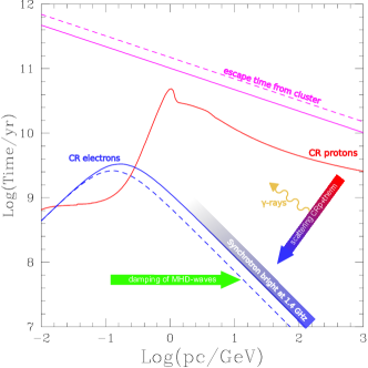
Figure 1: Lifetime of CR electrons (blue) and CR protons (red) in the ICM as well as their escape time (pink). Plotted for magnetic field strength of $1\,\mu\mathrm{G}$ (full) and $0.1\,\mu\mathrm{G}$ (dashed). Synchrotron bright energies are marked blue. Figure adapted and modified from Blasi et al. (2007a).

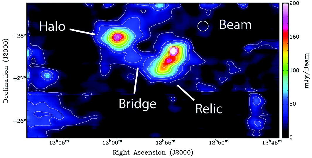
Figure 2: Complex non-thermal emission observed with GBT at 1.41 Ghz in Coma by Brown & Rudnick (2011). The beam size is roughly 360 kpc. Contours start at 20 mJy/beam and increase by 20 mJy/beam.

Today non-thermal phenomena in galaxy clusters are classified as radio halos, radio relics and mini halos (Feretti & Giovannini 1996). Radio halos are centered diffuse unpolarised objects found exclusively in clusters with disturbed X-ray morphology. Radio relics are thin, elongated, polarised radio structures offset from the cluster center. Both previous classes extend for one to two Mpc in size, while radio mini halos are usually limited to a few hundred kpc in the center of relaxed clusters. In this paper we focus on radio halos.

Independent measurements of the ICM magnetic field through Faraday rotation of intrinsic polarised radio sources (e.g. Bonafede et al. 2010) reveal field strengths of up to a few $\mu\mathrm{G}$ in the center of clusters, declining outwards. The field is observed to be highly tangled (Kuchar & Enßlin 2011), which is expected for a turbulent high beta plasma.

This is consistent with simulations, which predict efficient amplification by MHD turbulence as substructures merge with a parent cluster (Dolag et al. 2001, 2005; Dolag & Stasyszyn 2009). However Pfrommer & Dursi (2010) claim a radial magnetic distribution in the Virgo cluster. The origins of cluster magnetic fields are still debated (Widrow 2002).

Considering radio halos the observed field strengths imply a population of synchrotron bright CRe with energies of $>100\,\mathrm{GeV}$ in the whole cluster volume. It is well established that CRe are injected in shocks with Mach numbers larger than 5 through observations of supernova remnands (e.g. Eriksen et al. 2011). And on smaller scales AGN and SN shocks indeed contribute to the CRe content of a cluster. In contrast, accretion shocks during major mergers of clusters have low Mach numbers of $\approx 3$. The exact mechanism that might lead to an injection in these shocks is still debated (Spitkovsky 2008; Blasi 2010; Gargaté & Spitkovsky 2012). These primary CRe’s are believed to cause radio relics, which are associated with merger shocks in observations. However due to their geometry none of these mechanisms are volume filling. Therefore CRe would have to diffuse hundreds of kpc to form a radio halo.

Due to the low ambient thermal density of $n_{\mathrm{th}}<10^{-2}\,\mathrm{cm}^{-3}$, CRe have a classical mean-free-path of kpc in the ICM (Spitzer 1956). However particle motion faster than the Alvén speed in a plasma is known to cause plasma waves through the streaming instability (Wentzel 1974). These fluctuations in the plasma e-m-field themselves act as scattering agents in the medium and isotropise CR motions. Therefore CRe diffuse in a random walk through the cluster atmosphere, limiting the effective diffusion speed to the Alvén speed of $\approx 100\,\mathrm{km}/\mathrm{s}$.

Relativistic electrons are subject to a number of energy losses in the ICM as well (Longair 1994). The most important being inverse Compton scattering (IC), synchrotron radiation, bremsstrahlung and Coulomb scattering. Thus one can define an approximate life-time of these particles at an momentum $p$ as

$$t_{\mathrm{life}} =\frac{p}{\left|\frac{\mathrm{d}p}{\mathrm{d}t}\right|_{\mathrm{loss}}}.$$ (1)

In figure 1 we show this life-time for CRe and relativistic protons (CRp) as well as the escape time from the central ICM (modified from Blasi et al. 2007b).

It has been realised early on that these losses limit the diffusion length of radio bright CRe in the ICM to a few 10 kpc at best. It is unclear how a cluster-wide population of CRe can be maintained to produce a giant radio halo (Jaffe 1977). This is known as the life-time problem.

The existence of giant radio halos underlines the incompleteness of the physical picture described above. Indeed Dennison (1980) pointed out that relativistic protons have sufficiently long life-times to fill the cluster volume (see figure 1). CRp are likely to be injected alongside CRe into the ICM and can themselves inject synchrotron bright CRe in-situ through a hadronic cascade. Models relying on this mechanism are called hadronic or secondary models (see section 3).

In addition turbulent reacceleration might be able to explain giant radio halos (Jaffe 1977; Petrosian 2001; Brunetti et al. 2001). At low energies the synchrotron dark population of CRe with life-times of $>10^{9}\,\mathrm{yrs}$ can undergo stochastic reacceleration through damping of merger injected turbulence. This Fermi II like mechanism (Fermi 1949) lets CRe diffuse to higher momenta creating volume filling radio bright CRe. It may act on CRp as well (Brunetti & Blasi 2005; Brunetti & Lazarian 2011a). Effectively this mechanism can boost the radio brightness of a CRe population without altering the total CRe density by producing deviations from power-law spectra. This ansatz is realised in reacceleration models (see section 4).

Today the clear distinction between the two model classes can be considered a historic artefact as both processes certainly take place in the ICM to some degree. However, CRp have not been observed directly in the ICM so far and the efficiency of CRp injection in large scale ICM shocks is unclear. Hybrid particle in cell simulations suggest efficient CRp or CRe injection to be depending on the alignment of the magnetic field to the plane of the shock (Gargaté & Spitkovsky 2012). However, the low densities and mach numbers of large shocks in the ICM make these simulations just barely feasable. To this end the efficiency of CRp injection processes has not been firmly established.

In general the plasma physics in the exotic regime of the ICM presents a serious challenge to theorists and simulators. It should be considered that with mean free paths of $>1\,\mathrm{kpc}$ and collision times $>10^{6}\,\mathrm{yrs}$ in the ICM (e.g. Spitzer 1956; Sarazin 1999) particle-particle interactions are close to time and length scales relevant to radio halos. Therefore collisionality on kpc scales can not be mediated by particle-particle interactions. But observations of cold fronts and shocks confirm that the ICM is indeed a collisional plasma on smaller scales (Markevitch & Vikhlinin 2007). Collisionality can be recovered by plasma waves which results in very high Reynolds numbers of the ICM of $>1000$ or even $>10^{5}$ (Brunetti & Lazarian 2011b). Interestingly field-particle interactions happen on much smaller length and time scales in the ICM (debye length $\approx 2\times 10^{6}\,\mathrm{cm}$ (Schlickeiser 2002)).

To date the Coma cluster remains the prototypical cluster with non-thermal radio emission (figure 1, left). It has been studied extensively in the past and detailed studies on other clusters have been somewhat limited (Venturi 2011). However the situation will fundamentaly change with the arrival of new instruments like EMU+WODAN, LOFAR and later the SKA (Cassano et al. 2010; Cassano et al. 2012). At low frequencies of less than 100 MHz, radio halos are expected to be bright and ubiquitous, due to their steep emission spectrum. As increasingly more LOFAR stations see first light, studies of theoretical models for radio halos are particulary timely.

In the past decade theoretical research on halos has been devided along the lines of the two classical models. Numerical approaches used CRp dynamics and hadronic injection, sometimes with shock injection (Miniati et al. 2001; Dolag & Ensslin 2000; Ensslin et al. 2007; Pfrommer et al. 2008; Pinzke & Pfrommer 2010; Vazza et al. 2012; Hoeft et al. 2004; Hoeft et al. 2008; Brüggen et al. 2012; Keshet & Loeb 2010). Independently there were (semi-)analytic approaches on reacceleration models, sometimes including CRp (Petrosian 2001; Brunetti et al. 2001; Cassano & Brunetti 2005; Brunetti & Blasi 2005; Brunetti & Lazarian 2007, 2011a). Turbulence and magnetic fields have been studied extensively in the cluster context as well (Subramanian et al. 2006; Dolag et al. 1999; Vazza et al. 2008; Vazza et al. 2009, 2011; Iapichino & Niemeyer 2008; Maier et al. 2009; Iapichino et al. 2011; Ryu et al. 2008). However hadronic models have only recently been compared in detail to observations, while more complete approaches had not been considered in simulations yet (Donnert et al. 2010, 2010).

This report is organised as follows: We start with a general overview of the important observations of radio halos. We then show results from the comparison of hadronic models with these observations. We continue with an introduction to reacceleration models and conclude with the first simulations of CRe reacceleration in direct cluster collisions.

2 Observed Properties of Giant Radio Halos

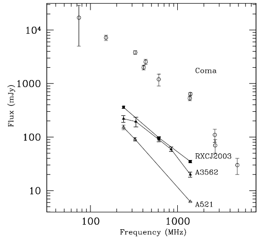
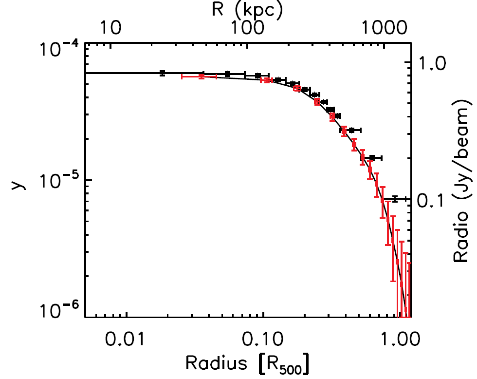
Figure 3: Left: Radio brightness at 1.4 GHz over bolometric X-ray luminosity for a sample of galaxy cluster. Upper limits of non-detections are marked as blue arrows, tentative detection from stacking as red limits (see Brown et al. 2011, and references therein). Middle: Radio spectra of 4 clusters (Venturi 2011). Right: Radial profile of Compton-y parameter (pressure along the LoS) and radio synchrotron emission in the Coma cluster out to $R_{500}$ (Planck Collaboration 2012).

Today roughly 50 radio halos are known, mostly at frequencies of 600 MHz and up (Giovannini et al. 2009; Feretti et al. 2012). These halos are all hosted in massive systems with disturbed X-ray morphology (Cassano et al. 2010). These systems form a correlation in X-ray luminosity and radio brightness with a slope of $\approx 1.8$ (figure 3 left panel). However in a complete X-ray sample these make only 30% of all systems (Venturi et al. 2007). Therefore for most clusters only upper limits in the radio are known (arrows in figure 3, left). Recently a first detection of these clusters has been claimed through a stacking analysis (Brown et al. 2011).

In the $\gamma$-ray regime, clusters remain not observed (Perkins 2008; Aharonian 2009; Ackermann 2010; Veritas Collaboration et al. 2012).

The Coma cluster has beed studied extensively in the past. Three observations at 1.4 GHz are commonly used to constrain radio synchrotron profiles of the cluster. It was debated (Pfrommer & Enßlin 2004) wether to use the steeper single-dish profiles from Deiss et al. (1997) or the flatter interferometer profiles from Govoni et al. (2001). However new single-dish GBT observations by Brown & Rudnick (2011) confirm the flat profile found previously by Govoni and present the deepest profile currently known.

For the Coma cluster (Thierbach et al. 2003) and a small number of other systems the spectrum of the diffuse emission is observed to be a power-law with a spectral index of 1.2 to 2.5. In figure 3, middle we show a few known examples from Venturi (2011). Halos with a synchrotron spectral index $\alpha_{\nu}>1.5$ (e.g. A521) are commonly named ultra-steep spectrum haloes. The Spectrum of the Coma cluster shows a break/steepening of the emission, which has important theoretical implications (see section 2.1). However differences in instrumentation and analysis might contribute to the total shape of the spectrum. Individual points were estimated with single-dish instruments as well as interferometers. While interferometers might lose diffuse flux because of limited UV-coverage, point source subtraction is complicated for single-dish data. Therefore the spectrum should be taken with a grain of salt.

The PLANCK satellite observed the Sunyaev-Zeldovich effect in a numebr clusters with unprecedented sensitivity and resolution. A correlation between the cluster Compton-y and radio luminosity was found from PLANCK data by Basu (2012), however without a clear indication for a bimodal distribution. This suggests that selection effects might contribute to the bimodality found in the X-ray-radio correlation.

In Coma, Planck Collaboration (2012) found that pressure and radio emission are tightly correlated up to $r_{500}\approx 1\,\mathrm{Mpc}$ (figure 3, right). Previous studies had shown that density and radio luminosity are correlated as well, however the scaling differs between clusters (Govoni et al. 2001).

Recent X-ray observations find a non-thermal pressure of $\leq 10\%$ in Coma (Churazov et al. 2012).

2.1 Direct Constrains on Models

The current observational status implies a number of constrains on the available models for a cluster-wide radio bright population of CRe :

1. The predicted radio emission has to be consistent with the observed profile (e.g. Brown & Rudnick 2011).

2. The non-thermal pressure by CRp, magnetic fields and turbulence in clusters may not exceed the non-thermal pressure constraint from the X-rays: $10\%$.

3. The observation of ultra steep spectrum halos like A512 indicates very steep CRe spectra of $>2$ (Brunetti et al. 2008). This implies either ”old” reaccelerated CRe or a CRp population with very steep spectral index in these clusters.

4. The non-detection of $\gamma$-rays constrains the amount of CRp in clusters.

5. The large number of non-detections in the radio regime suggests that radio halos are transient phenomena. Statistics roughly indicates that given the observed population a cluster may not stay on the correlation (i.e. be radio loud at 1.4 Ghz) for more than half a Gyr, with a transition period of roughly 200 Myr (Brunetti et al. 2009). The correlation reflects the structural self-similarity found in cluster properties, which is due to the self-similarity of the underlying DM halo and its gravitiational potential (Navarro et al. 1996).

3 Hadronic Models

Relativistic protons ($p/m_{\mathrm{p}}c>1\,\mathrm{GeV}$) might be injected in the ICM alongside CRe. CRp have long life-times and are trapped in the cluster volume (Berezinsky et al. 1997; Völk & Atoyan 1999). If their coupling to turbulence is inefficient their spectrum may only be slightly modified during their life-time so they are assumed to retain their power-law injection spectrum (Blasi & Colafrancesco 1999):

$$n_{\mathrm{p}}(p)\,dp =K_{\mathrm{p}}p^{-\alpha_{\mathrm{CRp}}}\,dp,$$ (2)

with a spectral index $\alpha_{\mathrm{p}}$. From accelerator data we know that CRp inject secondary CRe at GeV energies and $\gamma$-rays during collisions via a hadronic cascade (Dermer 1986):

$$p_{\mathrm{CR}}+p_{\mathrm{th}} \Rightarrow\pi^{0}+\pi^{+}+\pi^{-}+\mathrm{anything}$$

$$\pi^{\pm} \Rightarrow\mu+\nu_{\mu}$$

$$\mu^{\pm} \Rightarrow e^{\pm}+\nu_{\mu}+\nu_{e}$$

$$\pi^{0} \Rightarrow 2\gamma.$$

This allows to calculate the CR electron spectrum $n_{\mathrm{e}}(p)$ directly from the thermal density and the injection $Q({\bf r},p^{\prime},t)$ of CRe from the CRp spectrum 2. Under the assumption of slow varying MHD conditions in the ICM, injection and losses (eqs. 17+18) of CRe balance, the spectrum equillibrates and becomes stationary. The CR transport equation 16 can be simplified to:

$$\frac{\partial}{\partial p}\left(n_{\mathrm{e}}(p)\left.\frac{\mathrm{d}p}{\mathrm{d}t}\right|_{\mathrm{loss}}\right) =Q({\bf r},p,t)$$ (3)

The solution of this equation is then trivial (Dolag & Ensslin 2000):

$$n_{\mathrm{e}}(p) =\left|\frac{\mathrm{d}p}{\mathrm{d}t}\right|_{\mathrm{loss}}^{-1}\int\limits^{\infty}_{p}\,\mathrm{d}p^{\prime}\,Q({\bf r},p^{\prime},t).$$ (4)

Then the synchrotron emissivity follows analytically from the CRe for power-law spectra (Ginzburg & Syrovatskii 1965; Longair 1994; Rybicki & Lightman 1986; Pacholczyk 1970). For a spectrum of CRp like equation 2 the synchrotron emissivity scales like (e.g. Dolag & Ensslin 2000):

$$j_{\nu} \propto n_{\mathrm{th}}K_{\mathrm{p}}\nu^{-\alpha_{\nu}}\frac{B^{\alpha_{\nu}+1}}{B^{2}+B_{\mathrm{CMB}}^{2}},$$ (5)

with $\alpha_{\nu}=(\alpha_{\mathrm{e}}-1)/2=(2\alpha_{\mathrm{p}}-1)/3$ the spectral index of the radio synchrotron emission and $B_{\mathrm{CMB}}/(1+z)^{2}=3.2\,\mu\mathrm{G}$ the magnetic field equivalent of the CMB induced IC effect (Longair 1994). More elaborate models can be constructed which are based on a piecewise solution of the diffusion equation of CRp (Miniati et al. 2001) or adiabatic invariants (Ensslin et al. 2007). This has also been combined with a prescription for primary CRe and CRp injection in shocks (i.e. models for radio relics) (Pfrommer et al. 2008). Most models share the simplification of stationarity of the CRe spectrum obtained from the (sometimes non-stationary) CRp spectrum. In that case CR spectra and subsequent synchrotron spectra are limited to power-laws, sometimes in a number of energy bins. The coupling to turbulence is neglected in these works.

In hadronic models the injection efficiency for CRp and CRe in shocks is a free parameter. The $\gamma$-ray emissivity can be computed analytically as well (Pfrommer & Ensslin 2004).

The magnetic field in clusters is then often modelled relative to the thermal density (Dolag et al. 2001; Bonafede et al. 2010):

$$B(r) =B(0)\left(\frac{\rho(r)}{\rho(0)}\right)^{\eta_{\mathrm{mag}}}.$$ (6)

Free model parameters are then:

1. $K_{\mathrm{p}}(r)=X_{\mathrm{CRp}}(r)n_{\mathrm{th}}(r)$: the CRp normalisation is often given relative to the thermal density ($X_{\mathrm{CRp}}\in[10^{-5},0.1]$) or simulated directly in a numerical approach. It is constrained by the synchrotron profile and has to be consistent with the observed non-thermal pressure and $\gamma$-ray limits.

2. $\alpha_{\mathrm{p}}\in]2.0,3.0[$: the CRp spectral index translates to CRe and synchrotron spectal index and is therefore constrained by observed radio halo spectra. The spectral index enters the $\gamma$-ray emissivity as well. The observed break in the radio spectrum of Coma is often (falsely) attributed to the SZ-decrement. This is then combined with a flatter $\alpha_{\mathrm{p}}$ and a flat magnetic field to fit $\gamma$-ray constrains (Veritas Collaboration et al. 2012). We will discuss this in section 3.2.1.

3. $B(0)\in[1,10]\,\mu\mathrm{G}$: the cluster magnetic field normalisation is directly constrained from RM observations, equipartition arguments and simulations.

4. $\eta_{\mathrm{mag}}\in[0,1]$: the cluster magnetic field scaling relative to the thermal density. While being constrained by the same observations as the normalisation some models assume (nearly) flat magnetic fields.

3.1 Simulations & CR formalism

Exemplary we show here results from constrained cosmological MHD simulations published in Donnert et al. (2010, 2010). These are consistent with analytic comparisons with newest data (Brunetti et al. 2012).

The constrained power-spectrum initial conditions produces matter structures which on scales of a few Mpc (clusters) can be identified with their real counterparts (Mathis et al. 2002). The magnetic field was initialised from galactic outflows as shown in Donnert et al. (2009). The radio emission is then estimated with an analytic approach to the CR physics: we use the high energy approximation to the p-p cross-section in Brunetti & Blasi (2005) to compute the synchrotron emissivity of a cluster. We estimate the $\gamma$-ray brightness from our models using the formalism by Pfrommer & Ensslin (2004).

We model the radial profile of CRp normalisation $X_{\mathrm{CRp}}(r)$ relative to the thermal density as:

$$X_{\mathrm{CRp}}(r) =X_{\mathrm{CRp}}(0)\left(\frac{\rho(r)}{\rho(0)}\right)^{-\eta_{\mathrm{CRp}}}.$$ (7)

We will fix the normalisation $X_{\mathrm{CRp}}(0)$ and the scaling $\eta_{\mathrm{CRp}}$ in the next section to fit the observed radio profile. The proton spectral index $\alpha_{\mathrm{CRp}}$ is another free parameter which we will constrain from the observed spectrum. The magnetic field is taken from the simulation and is roughly consistent with observations in Coma with $\eta=0.5$ and $B_{0}\approx 1\,\mu\mathrm{G}$ (Bonafede et al. 2010). The result is shown in figure 4, where we the magnetic field profile is plotted alongside the square root of the density.

Figure 4: Radial profile of magnetic field strength and square root of the density (dashed) of the simulated cluster. The smallest resolution scale $2h_{\mathrm{sml}}$ is marked as dotted line.

3.2 Results

In this section we will focus on the Coma cluster first. We show how multi-frequency observations constrain the hadronic model. An overview of the parameters used can be found in table 1. Then we show the P14-LX correlation for a sample of simulated galaxy clusters and comment on the implications of the PLANCK correlation between thermal pressure and radio emission in Coma.

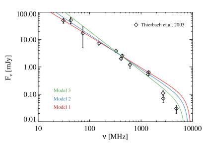
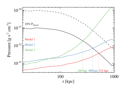
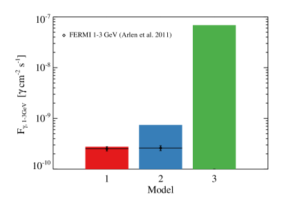
Figure 5: Top left: Observed radio spectrum in the Coma cluster, black diamonds (Thierbach et al. 2003). Spectra of three hadronic models with $\alpha_{\mathrm{CRp}}=2.3,2.6,2.9$ and $\eta_{\mathrm{CRp}}=1.4,1.4,2.4$. The SZ-decrement has been included pixel by pixel from the observed PLANCK map (Brunetti et al. in prep.) . Top right: Radial profile of radio synchrotron emission in Coma at 300 MHz (top, normalised, Brown & Rudnick 2011) and 1.4 GHz (bottom, Deiss et al. 1997). In colors the three models with a CRp scaling to fit the conservative profile at 1.4GHz (red, blue) and the deep profile at 300 MHz (green). Bottom left: Non-thermal pressure constraint in Coma (black line, Churazov et al. 2012) and non-thermal pressure from the numerical models. Bottom right: Fermi upper limits at $\alpha_{\mathrm{CRp}}=2.3,3.5$ from Veritas Collaboration et al. (2012) and expected $\gamma$-ray flux from the three numerical models.

3.2.1 Coma: Spectrum & SZ-decrement

Hadronic models predict a power-law synchrotron spectrum (equation 5), in contrast to the observed break in the Coma spectrum. It has been argued that the break can be explained by the Sunyaev-Zeldovich decrement in the unavoidable CMB radio signal measured alongside the actual halo emission (Ensslin 2002; Pfrommer & Ensslin 2004). The SZ-decrement is the modification of the CMB thermal emission by the clusters Sunyaev-Zeldovich effect at halo frequencies (Sunyaev & Zeldovich 1980). This is not connected to the halo emission, but contaminates the total emission measured from the halo. Naturally the influence is limited to the region of the radio halo only. However Ensslin (2002) considered the flux from a region more than twice the size of the radio halo (5 Mpc radius), therefore overestimating the decrement.

Due to the high resolution of the PLANCK measurements, the SZ-decrement can now be directly estimated from observations. It is instructive to assume three spectral indices: $\alpha_{\mathrm{CRp}}=2.3$ and $\alpha_{\mathrm{CRp}}=2.6$, as well as $\alpha_{\mathrm{CRp}}=2.9$. In figure 5, top left we show the Coma radio spectrum and three analytical hadronic models with these spectral indexes, including the SZ-decrement from the PLANCK data (preliminary results from Brunetti in prep.). The spectra are normalised to 300 MHz, where the influence of the decrement is negligible. Only the last model leads to a marginally consistent fit of the observed radio spectrum. A hadronic model with spectral index of 2.6 is already more the a factor of two away from the observations. Therefore even given the uncertainties in the observations (see section 2) the SZ-decrement is not able to reproduce the break for indizes smaller than 2.6.

Parameter	Model 1	Model 2	Model 3
$\alpha_{\mathrm{CRp}}$	2.3	2.6	2.9
$\eta_{\mathrm{CRp}}$	1.4	1.4	2.4
$X_{\mathrm{CRp}}(0)$	0.002	0.006	0.006
$B_{0}[\mu\mathrm{G}]$	1	1	1
$\eta_{\mathrm{mag}}$	0.5	0.5	0.5
fit $\nu\,\mathrm{MHz}$	1400	1400	300

Table 1: Parameters and values for the three numerical models used in this comparison.

3.2.2 Coma: Radial Profiles

The total radio flux and radial profile of the emission in Coma can be used to constrain the amount of CRp in the cluster, i.e. $X_{\mathrm{CRp}}(r)$. We set the scaling according to equation 7 to fit (table 1) the observed radio profile at 1.4 GHz for model one and two (Deiss et al. 1997), and 300 MHz for model three (Brown & Rudnick 2011). The fits are shown for all three models in figure 5, top right graph. This implies $\eta_{\mathrm{CRp}}=1.4$ for the models with small spectral index and $\eta_{\mathrm{CRp}}=2.4$ for the other one. The total luminosity of the models is fixed at 1.4 GHz to be $640\pm 5\,\mathrm{mJy}/\mathrm{arcsec}^{2}$ following Deiss et al. (1997).

The first two models use the older radio profile at 1.4GHz. The is very conservative estimates as at low frequencies the halo is observed to be much flatter and larger (Venturi et al. 1990; Govoni et al. 2001; Brown & Rudnick 2011). Indeed the third model uses the state-of-the-art radio observation of the COMA cluster and models the best constrains available on the radio halo problem today.

CRp exert non-thermal pressure to the ICM, similar to turbulence and magnetic fields. Recent observational studies on Coma set an upper limit to non-thermal pressure of 10 % in the cluster (Churazov et al. 2012). For comparison we plot in figure 5 bottom left, the thermal pressure profile (dashed line) alongside the 10% limit (full line) and the non-thermal pressure of the three models (red, green, blue). The pressure constrain is violated at radii of $r_{10}\approx 510,400,260\,\mathrm{kpc}$, while the observed radio halo at 300 MHz extends to $\approx 1000\,\mathrm{kpc}$. Therefore observations imply considerable non-thermal pressure at large radii for hadronic models. For the Coma cluster $r_{10}$ could be increased by flatter magnetic field models for flat CRp spectra. However this becomes less consistent with magnetic fields derived from observed rotation measures.

The situation becomes increasingly problematic when considering halos like A512. The steep spectrum of these objects require abundant CRp contents to reproduce the emission at lowest frequencies. Observed synchrotron spectra of $\alpha_{\nu}\approx 2.1$ imply $\alpha_{\mathrm{CRp}}=3.5$. This results in non-thermal pressures of more than 50 % within 3 core radii (Brunetti et al. 2008; Dallacasa et al. 2009).

3.2.3 $\mathbf{\gamma}$-ray brightness

Observations of $\gamma$-ray emission from hadronic collisions in the ICM are an independent way of constraining the CRp content in clusters. Newest upper limits in this frequency band come from FERMI and VERITAS, while the former ones are most constraining (Veritas Collaboration et al. 2012).

In figure 5 bottom right, we show the most constraining upper limits from FERMI ($\alpha_{\mathrm{CRp}}=2.3,2.5$) as well as our three numerical models. Only the first model with the flattest CRp spectrum is marginally consistent with the newest $\gamma$-limits given the simulated magnetic fields. The other two steeper models violate the observed limits. Again the situation could be eased by a stronger and flatter magnetic field profile in the case of flat CRp spectra. The steep $\alpha_{\mathrm{CRp}}$ model however can be considered excluded by $\gamma$-ray observations. It is the only one roughly consistent with the observed radio spectrum though.

3.2.4 Radio - X-ray Correlation

Figure 6: Full sky map of radio flux from a hadronic model with $X_{\mathrm{CRp}}(r)=1\%$ and $\alpha_{\mathrm{CRp}}=2.6$ in a cosmological MHD simulation.

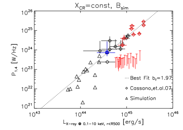
Figure 7: Radio brightness at 1.4GHz over X-ray brightness between 0.2 and 2.4 keV for 16 clusters with $X_{\mathrm{CRp}}(r)=1\%$ and $\alpha_{\mathrm{CRp}}=2.6$. Observed halos as diamonds from (Cassano et al. 2007) and upper limits from (Venturi et al. 2007).

Figure 7 shows 16 simulated clusters from the cosmological simulation in the $P_{14\mathrm{GHz}}-L_{\mathrm{X-ray}}$ plane (triangles, $X_{\mathrm{CRp}}=1\%$, $\alpha_{\mathrm{CRp}}=2.6$). Overplotted are the observed correlation (dotted line), observed radio halos (red & white diamonds, Venturi et al. (2007)) and upper limits (red lines). The observed correlation is well reproduced by the largest clusters in the simulated sample.

However the brightness distribution from the simulation is not bimodal: all large clusters show significant radio emission. This is an intrinsic prediction of hadronic models. As CR protons are trapped in the cluster volume they accumulate in the ICM. In figure 6 we show a full sky projection of the radio synchrotron emission from the simulation using the $X_{\mathrm{CRp}}=const$ model and the simulated magnetic field. Every cluster shows diffuse radio emission. The radio sky predicted by this model is shown in figure 6.

3.3 Summary

Given our simulated magnetic fields, hadronic models:

1. reproduce the $P_{14\mathrm{GHz}}-L_{\mathrm{X-ray}}$ correlation, but in the case of classical models fail the bimodal distribution of the population.

2. do not reproduce the deepest observed radio profile in Coma within the non-thermal pressure constrains. This could be eased using a flatter and stronger magnetic field distribution. However this tends to be not consistent with observed RM measures in the Coma cluster.

3. are not consistent with present upper limits in the $\gamma$-ray regime when reproducing deepest Coma radio observations and its radio spectrum. Models using $\alpha_{\mathrm{CRp}}=2.3$ are indeed consistent with these limits if the 1.4GHz profile is fitted. However they do not fit the Coma spectrum (figure 5, top left).

4. do not reproduce the break in the Coma spectrum when $\alpha_{\mathrm{CRp}}<3$.

The observed constrains present serious challenges for hadronic models. The observed spectrum of the Coma cluster is impossible to fit without violating non-thermal pressure constrains and $\gamma$-ray limits. In the most recent attempts Veritas Collaboration et al. (2012); Zandanel et al. (2012) report a good fit to the observed constrains. However in these papers Coma is modelled with $\alpha_{\mathrm{CRp}}=2.1-2.4$ at 1.4 GHz only !

The PLANCK Compton-y - Radio Correlation:

The situation can be presented most elegantly from the observed Compton-y - 300 MHz radio profile correlation in Coma (Mazzotta & Planck Collaboration 2012). In the center of the cluster, the fit in figure 5 (and most other hadronic models) predict $X_{\mathrm{CRp}}\approx 10^{-3}-10^{-2}$ (depending on the CRp spectral index) to reproduce the luminosity profile locally. At the outer radii ($300<r<1000\,\mathrm{kpc}$), where $B<<B_{\mathrm{CMB}}$, PLANCK found:

$$y_{\mathrm{Compton}} \propto j_{\mathrm{1.4GHz}}(r).$$ (8)

The Compton-y parameter measures pressure, so:

$$y_{\mathrm{Compton}}(r) \propto P\propto n_{\mathrm{th}}T,$$ (9)

$$j_{\mathrm{1.4GHz}} \propto X_{\mathrm{CRp}}n_{\mathrm{th}}^{2}B^{2}.$$ (10)

The temperature profile in clusters is roughly constant with radius, and we have

$$X_{\mathrm{CRp}} \propto n_{\mathrm{th}}^{-1}B^{-2},\quad\mathrm{and}$$ (11)

$$n_{\mathrm{th}} \propto(1+r^{2}/r_{\mathrm{c}}^{2}),$$ (12)

for $r\leq r_{500}$. It follows from the PLANCK correlation that $X_{\mathrm{CRp}}\propto(1+r^{2}/r_{\mathrm{c}}^{2})$, even for a flat magnetic field. In Coma $r_{\mathrm{c}}\approx 0.3\,r_{500}$, so $X_{\mathrm{CRp}}$ has to increase by a factor of 10 in this case. If $\alpha_{\mathrm{CRp}}>2.9$ then $X_{\mathrm{CRP}}\approx 0.01$ and the non-thermal pressure constraint of 10% is violated at 1Mpc even for flat magnetic field models.

However observed rotation measures suggest $B\propto n_{\mathrm{th}}^{1-0.5}$ (Bonafede et al. 2010). Here the increase is a factor of 100 to 1000 and the non-thermal pressure constraint is violated in any case.

3.4 A Comment on Non-classical Hadronic Models

Recently Enßlin et al. (2011) proposed a model based on CRp transport in the ICM in an attempt to explain the bimodal distribution of halos in the hadronic framework. In this model the bimodality reflects two modes of CRp transport in clusters:

• During mergers CRp transport is dominated by convection through turbulent motions. CR protons are effectively stored between converging magnetic field lines and dragged along the turbulent motions. These motions are injected at a scale of the core radius and induce an MHD cascade of cluster-wide turbulence. This way the CRp density in the center of clusters is increased. The resulting flatter $X_{\mathrm{CRp}}$ profile leads to the observed radio bright clusters.

• After turbulence has decayed CRp transport is supposed to be dominated by super-Alvenic streaming of CRp along the magnetic field lines. If small scale turbulence is not driven by external processes the streaming instability is the only source of fluctuations at that scale. Scattering of CRs on these fluctuations limits the diffusion speed to the Alven speed (Wentzel 1974). Specifically the isotropisation of CRp for small pitch angles (i.e. reversal of direction along the field) is mediated by scattering with large modes (i.e. mirror interactions) (Felice & Kulsrud 2001). However these modes are damped efficiently by the ICM plasma through the ion cycloton resonance. Enßlin et al. (2011); Holman et al. (1979) argue that this way the streaming instablity is inefficient to generate modes at small pitch angles. This would allow streaming motions along the field lines comparable to the sound speed (highly super-Alvenic). Eventually this tends to remove CRp from the cluster center and flatten the CRp profile of the cluster. Subsequently the radio brightness declines. This process might as well be able to explain the steepening of the radio spectrum as a superposition of different CRp populations.

However the assumption of streaming velocities higher than the Alven speed had been rejected earlier for CRe and only lead to the cooling time dilemma. We therefore see three problems in the argumentation presented in (Enßlin et al. 2011; Holman et al. 1979) and above:

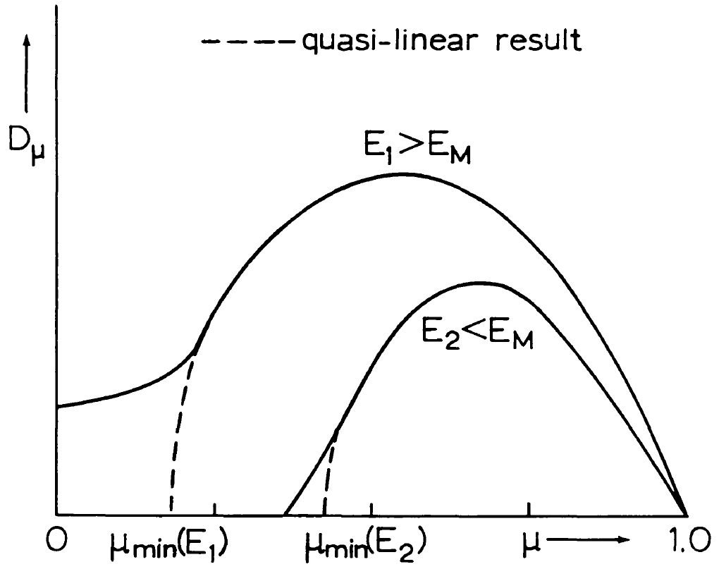
Figure 8: Diffusion coefficient over pitch angle in radians (Achterberg 1981). The quasi-linear result is shown dashed, the non-linear result as full curve. In clusters $E_{1}>E_{\mathrm{M}}$.

• Cosmological simulations show that even in relaxed clusters, structure formation causes a constant infall of small halos into the ICM, driving turbulence. The ICM itself is not a classical collisional plasma. Probably collective effects mediate collisionality, which implies very high Reynolds numbers of the plasma (Brunetti & Lazarian 2011b). Therefore the infall of structures always causes turbulence on kpc scales which is dissipated at sub-pc scales. This is in contrast to the non-classical hadronic approach which relies on small modes generated exclusively by the streaming instability. Even though damping processes are ill constrained in the ICM it is likely that externally driven turbulence is always present at some level on the damping scale of CRp.

• Holman et al. (1979) argue that at pitch angles of $\mu<2\,\mathrm{deg}$ turbulence is completely absent due to the strong damping by the thermal ions. However even in the absense of external driving, turbulence is constantly injected on a range of scales by CRp through the streaming instability. Due to mode coupling these motions will form a cascade and develop a break with finite steepness at the wavelength of interest (Spangler 1986; Schlickeiser 2002). Therefore turbulence is unlikely to be completely absent, even if ion cycloton damping is stronger than the growth rate from the streaming instability.

• Holman et al. (1979) calculate the diffusion coefficient in the quasi linear regime. In that formalism the resonance function $R_{j}(\vec{k},\omega_{j})$ is approximated by a delta function (e.g. Schlickeiser 2002):

  $$R_{j}({\bf k},\omega_{j}) =\pi\delta(v\mu k_{\parallel}-\omega_{\mathrm{R,j}}+n\Omega).$$ (13)

  However, this approximation is only valid if $\Gamma_{j}\rightarrow\infty$, i.e. damping of plasma modes is negligible (Melrose 1980). This is not the case in the situation considered here. Ion cycloton damping obviously has to be considered, because it is supposed to dominate at small pitch angles. The correct resonance function is of Breit-Wigner type (e.g. Schlickeiser 2002):

  $$R_{j}({\bf k},\omega_{j}) =\frac{\Gamma_{j}({\bf k})}{\Gamma^{2}_{j}({\bf k})+(v\mu k_{\parallel}-\omega_{\mathrm{R,j}}+n\Omega)}$$ (14)

  Considering this resonance function the diffusion coefficient has been investigated in non-linear theoretical approaches (Dupree 1966; Weinstock 1970, 1969; Völk 1973; Ben-Israel et al. 1975; Goldstein 1976; Achterberg 1981; Jones et al. 1978; Yan & Lazarian 2008). The resulting diffusion coefficient ($D_{\mu}$) is consistent between authors. We show in figure 8 the result from Achterberg (1981) which does not vanish for $\mu\rightarrow 0$, in the case of fully relativistic particles. CR scattering through $\mu=0$ appears not to be a problem in the correct non-linear approach.

We conclude that CR streaming is not important in galaxy clusters.

4 Reacceleration Models

The ICM thermal plasma might be dominated by field-particle interactions to establish the observed collisionality of the plasma. This can be seen when comparing particle-particle and particle-field interactions: In a cluster, particle collision lengths are $>1\,\mathrm{kpc}$ and the speed of a particle in the collisionless regime is the sound speed, $\approx 10^{8}\,\mathrm{cm}/\mathrm{s}$. However the debye length is of the order of $20\,\mathrm{km}$ (Schlickeiser 2002). That means every charged particle is coupled to $\approx 10^{6}$ neighbouring particles through its em-field, with quasi instantaneous interaction speed (the speed of light). In contrast the time between collisions is $10^{21}\,\mathrm{cm}/3\times 10^{8}\mathrm{cm}/\mathrm{s}\approx 1\,\mathrm{Myr}$.

One may consider, that major mergers drag $10^{62}\,\mathrm{erg}$ of kinetic energy into the ICM. The most part is dissipated through shocks into heat, which is prominently seen in radio relics (e.g. Vazza et al. 2009, 2012). Additionally, vortical motions, shear flows and instabilities efficiently drive turbulence in the ICM (Subramanian et al. 2006), because of its high Reynolds number. This amplifies magnetic fields to $\mu G$ values (Dolag et al. 2001; Donnert et al. 2009; Beck et al. 2012). Furthermore, turbulent modes (local field fluctuations) resonantly couple to the cosmic-ray electrons in the ICM on pc scales (Schlickeiser 2002). This way a synchrotron dark, long-lived population of CRe can diffuse throughout a cluster, and is accelerated to synchrotron bright energies by turbulence, on a time-scale shorter than the life-time of radio halos (Petrosian 2001; Brunetti et al. 2001; Schlickeiser et al. 1987).

4.1 Dynamics of the CRe population

Models involving reacceleration do not assume stationarity of the CR population. Therefore the analytical formalism based on the stationarity condition, eq. 3, can not be used in this framework. Again the population of cosmic-rays is described by its isotropic spectral density $n(p,t)$ in momentum space. The dynamics of this spectrum is determined by the interplay between cooling, due to radiative and Coulomb losses, and acceleration, due to turbulence (figure 1,left). The momentum transport is governed by a Fokker-Planck equation (16), in which these processes are realised as coefficients. The loss terms (eqs. 17, 18) define a cooling time scale which is given by equation 1, and is of the order of $10^{8}\,\mathrm{yrs}$ for synchrotron bright CRe in the ICM (see section 1).

The coupling to turbulence through resonant scattering on plasma waves is realised through the $D_{\mathrm{pp}}$ coefficient (eq. 23), which defines an acceleration time scale (e.g. Cassano & Brunetti 2005):

$$t_{\mathrm{acc}}^{-1} =4\frac{D_{\mathrm{pp}}}{p^{2}}.$$ (15)

Stochastic acceleration is efficient only, if this time scale is comparable or smaller than the cooling time scale in the medium. For the ICM this is true, when the local turbulent velocity is of the order of $\approx 300\,\mathrm{km/s}$ on scales of $50\,\mathrm{kpc}$.

4.1.1 The transport equation

The change of the spectrum $n(p)$ in momentum space is described by a Fokker-Planck equation. It follows from the relativistic Maxwell-Vlasov system of equations (see Schlickeiser 2002, and references therein). Here one neglects the spatial diffusion of cosmic-rays in the ICM for reasons layed out in section 3.4 (Wentzel 1974).

$$\frac{\partial n(p,t)}{\partial t} =\frac{\partial}{\partial p}\left[n(p,t)\left(\left|\frac{\mathrm{d}p}{\mathrm{d}t}\right|_{\mathrm{rad}}+\left|\frac{\mathrm{d}p}{\mathrm{d}t}\right|_{\mathrm{ion}}-\frac{2}{p}D_{\mathrm{pp}}(p)\right)\right]$$

$$+\frac{\partial}{\partial p}\left[D_{\mathrm{pp}}(p)\frac{\partial n(p,t)}{\partial p}\right]+Q_{\mathrm{e}}(p,t).$$ (16)

Conceptually this is a non-linear momentum diffusion equation. Setting $D_{\mathrm{pp}}=0$, one recovers the usual diffusion equation with the loss terms as positive definite diffusion coefficient. This leads to diffusion to lower momenta, i.e. cooling. For $D_{\mathrm{pp}}\neq 0$ this diffusion coefficient is modified and can become negative, leading to diffusion to higher momenta, i.e. heating. Additionally, the second term on the right hand side describes a non-linear broadening of the distribution. The evolution of a spectrum is shown in figure 11, left for constant injection of power-law CRe at momenta $p\in[50,10^{5}]\,\mathrm{m}_{\mathrm{e}}\mathrm{c}$.

The injection of CRe

in the Fokker-Planck equation is described by an injection function $Q(p,t)$. Possible injection sources include shock acceleration, hadronic processes, reconnection, AGN and galactic outflows (Blasi et al. 2007; Lazarian & Brunetti 2011). In general these processes are found to inject power-law distributions of CRe into the ICM (see e.g. Blasi 2010, for details).

The loss terms

due to inverse Compton scattering with CMB photons and synchrotron radiation and Coulomb losses at $z=0$ take the form (Cassano & Brunetti 2005):

$$\left.\frac{\mathrm{d}p}{\mathrm{d}t}\right|_{\mathrm{rad}} =-4.8\times 10^{-4}p^{2}\left[\left(\frac{B_{\mu G}}{3.2}\right)^{2}+1\right],$$ (17)

$$\left.\frac{\mathrm{d}p}{\mathrm{d}t}\right|_{\mathrm{ion}} =-3.3\times 10^{-29}n_{\mathrm{th}}\left[1+\mathrm{ln}\left(\frac{\gamma}{n_{\mathrm{th}}}\right)/75\right],$$ (18)

where $B_{\mu\mathrm{G}}$ is the magnetic field in micro Gauss, $n_{\mathrm{th}}$ the number density of thermal particles and $\gamma$ the Lorentz factor.

One may observe that synchrotron emission can be described with an effective magnetic field in the IC formula. This stems from the fact that IC and synchrotron mechanisms use the same quantum-mechanical scattering process (Longair 1994). They are dominant at higher momenta ($p>10^{3}\,\mathrm{m}_{\mathrm{e}}\mathrm{c}$). Ionisation losses and Coulomb scattering depend on the thermal number density of particles in the ICM $n_{\mathrm{th}}$ and are dominant in the low energy regime ($p<10^{2}\,\mathrm{m}_{\mathrm{e}}\mathrm{c}$).

The momentum diffusion coefficient

follows from a pertubative approach to the relativistic Maxwell-Vlasov system of equations. Here it is assumed that the change of the field perturbation by the particle can be neglected. This is referred to as quasi-linear-theory. The rigorous derivation is lengthy, see Schlickeiser (2002) for details. We follow here a more physical the approach by Brunetti & Lazarian (2007).

The $D_{\mathrm{pp}}$ coefficient describes the interaction of cosmic-rays with turbulence in a plasma. Turbulent fluctuations manifest in a plasma, amongst others, in fluctuations of the electric and magnetic field. In the ICM these fluctuations can be damped by cosmic-rays, similar to how a dielectric damps an infalling light-wave.

The dielectric tensor describes the action of the medium/CRs on the fluctuating e/m-fields. In the core of this process is the resonance condition (eq. 19), which describes the coupling of the particle population to the e/m-fields. However turbulence is a statistical process and the turbulent fluctuations are better described by a spectrum in $k$-space. This spectrum evolves according to a damped diffusion equation (eq. 21). To describe the action of the dielectric on the damping of the waves the dielectric tensor has to be translated to a damping coefficient (eq. 20). Using detailed balancing and a Kraichnan spectrum, the diffusion coefficient (eq. 23) can then be derived from an energy argument (eq. 22).

Brunetti & Lazarian (2007) consider only the scattering by fast compressive turbulent modes. This is the least efficient coupling, which makes this a conservative approach. Alven waves have been considered in e.g Brunetti et al. (2004) and Brunetti & Blasi (2005), but require CR protons and their back-reaction on the spectrum.

In the presence of compressible low-frequency MHD-waves with an energy spectrum $W(k)$, relativistic particles with velocity $v$ in a magnetic field are accelerated by electric field fluctuations. In quasi-linear theory this gyroresonant interaction applies for the resonance condition (Melrose 1968):

$$\omega-k_{\parallel}v_{\parallel}-n\frac{\Omega}{\gamma} =0,$$ (19)

with $\omega$ the frequency of the wave, $k_{\parallel}$ and $v_{\parallel}$ the wave-vector and particle velocity parallel to the magnetic field, $\Omega$ the Larmor frequency, $\gamma$ the Lorentz factor and $n$ the resonance order. Here only $n=0$ case is considered (Transit time damping), which requires effective pitch-angle isotropisation of the particles by other processes.

The resonance condition (19) can be used to derive the damping rate $\Gamma$ of turbulence from the dielectric tensor $K_{ij}^{\mathrm{a}}$ in the limit of long wavelengths. Note that here indeed one is allowed to use the quasi-linear approximation equation 13, because the damping is very small. The damping rate then follows from the dielectric tensor via (Melrose 1968):

$$\Gamma =-i\left(\frac{E^{*}_{i}K_{ij}^{\mathrm{a}}E_{j}}{16\pi W(k)}\right)_{\omega_{i}=0}\omega_{\mathrm{r}},$$ (20)

where $E_{i}$ are the electric fields, $\omega_{\mathrm{r}}$ is the real part of the frequency of the fluctuating field, and $\omega_{i}$ its imaginary part.

The turbulence spectrum follows the damped diffusion equation:

$$\frac{\partial W_{\mathrm{k}}(t)}{\partial t} =\frac{\partial}{\partial k}\left(D_{\mathrm{kk}}\frac{\partial W_{\mathrm{k}}(t)}{\partial k}\right)-\sum\limits_{i=1}^{N}\Gamma^{i}(k)W_{\mathrm{k}}(t),$$ (21)

with the diffusion coefficient due to mode coupling $D_{\mathrm{kk}}=k^{2}/\tau_{\mathrm{s}}$, $\tau_{\mathrm{s}}$ the spectral energy transfer time. Here $i$ sums over all damping processes of turbulence in the plasma. For the high-$\beta$ ICM thermal particles and CRp argueably do not damp fast modes efficiently. Therefore we only consider CRe damping here ($N=1$).

The argument of detailed balancing then states that the energy lost by the turbulent waves below a scale $l$ due to CRe damping equals the energy change in the relativistic particles. It relates the total energy in a mode $W(k)\,\mathrm{d}k$ to the particle spectrum (Eilek 1979; Achterberg 1981):

$$\int\mathrm{d}p\,E_{\mathrm{CRe}}\left(\frac{\partial f_{\mathrm{CRe}}(p)}{\partial t}\right)=\int\mathrm{d}k\,\Gamma_{\mathrm{CRe}}(k,\theta)W(k).$$ (22)

From this argument $D_{\mathrm{pp}}$ can be found:

$$D_{\mathrm{pp}} \approx 9\times 10^{-8}p^{2}\frac{v_{\mathrm{turb}}^{4}}{c_{\mathrm{s}}^{2}l}\eta_{\mathrm{turb}}^{2}$$ (23)

for Kraichnan turbulence $P(k)\propto k^{-3/2}$ and an energy fraction in magneto-sonic waves $\eta_{\mathrm{turb}}$.

4.2 Model Parameters

As reacceleration models are non-stationary, all parameters have to be estimated as a function of time. One may model the thermal quantities with the usual isothermal beta model. This leaves the following model parameters:

• Magnetic field distribution, i.e. $B_{0}(t)$ and $\eta_{\mathrm{B}}(t)$.

• Spectral distribution of turbulence $W(t)$: e.g. a power-law with index $\alpha_{\mathrm{turb}}$, cut-off $k_{\mathrm{min}}$, $k_{\mathrm{max}}$ and normalisation $W_{0}(t)$. For Kraichnan turbulence this translates to eq. 23 with the turbulent velocity $v_{\mathrm{turb}}$ at scale $l$.

• The fraction of turbulence in magneto-sonic waves $\eta_{\mathrm{turb}}\in[0.01,0.5]$. This parameter is not well constrained, but given the theoretical uncertainties in the coupling (see the motivation of $D_{\mathrm{pp}}$ above) values between 0.01 and 0.5 seem acceptable.

• A source of CRe, i.e. $Q(t)$.

The time evolution of the particle spectrum as well as the resulting synchrotron emission have to be estimated numerically.

While semi-analytical models have been applied successfully in the past (e.g. Fujita et al. 2003) the complexity of the problem really requires a fully numerical approach.

4.3 First Simulations

We show results from a first numerical study of reacceleration in cluster mergers (Donnert et al. 2012). This work makes use of the MHDSPH code GADGET3 (Springel 2005; Dolag & Stasyszyn 2009) and a model for isolated cluster collisions (Donnert in prep., section 4.3.2). We self-consistently follow the collisionless dynamics of dark matter (DM), and the gas in the MHD-approximation. This simulates the temperature, density and magnetic field distribution of the merger over time. In addition the following parameters are used:

• the magnetic field is setup with $\eta_{\mathrm{mag}}=1$

• Turbulence follows a Kraichnan spectrum below the numerical resolution, so the diffusion coefficient equation 23 is used. Above the resolution scale turbulence is computed explicitely by the code.

• A numerical model for smoothed particle hydrodynamics (SPH) turbulence gives $v_{\mathrm{turb}}$ on the kernel scale $l=2h_{\mathrm{sml}}$. Here $h_{\mathrm{sml}}$ is the compact support of the kernel.

• $\eta_{\mathrm{turb}}=0.2$

• CRe are assumed to be constantly injected into the ICM. The injection coefficient is modelled as:

  $$Q_{\mathrm{e}}(\gamma,t)=K_{e}\varepsilon_{\mathrm{th}}^{2}\gamma^{-2}\sqrt{1-\frac{\gamma}{10^{5}}}(1-\frac{50}{\gamma}),$$ (24)

  which is a power-law with smooth cut-offs at $\gamma=p/\mathrm{m}_{\mathrm{e}}c=50,10^{5}$. As the injection scales as the thermal energy density $\varepsilon_{\mathrm{th}}$ it is equivalent to an hadronic injection. $K_{\mathrm{e}}\approx 10^{-4}$

4.3.1 Fokker-Planck Code

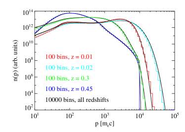
Figure 9: Comparison of CRe spectra from our code (colours) using 100 gridcells with another code (black) used in Cassano & Brunetti (2005) with 10000 cells.

In post-processing to the simulation we follow dynamics of the CRe spectrum by solving the transport equation 16 (Donnert in prep.) in parallel. We linearly interpolate between simulation outputs every 10 Myr and use a conservative timestep of 1 Myr in the code. The Fokker-Planck coefficients are computed from equations 17, 18, 23 and 24 using the thermal and turbulence properties from the simulation.

We sample the CRe spectrum in 100 logarithmic bins between $p/m_{\mathrm{e}}c=1$ and $10^{6}$. We realise open boundary conditions with the method from Borovsky & Eilek (1986). We use the method of Chang & Cooper (1970) to compute the time evolution of the spectrum. They derive a first-order accurate adaptive upwind scheme which can be analytically shown to:

• be unconditionally stable

• guarantee positivity

• converge to the steady-state solution.

• conserve particle number.

This means it is ideally suited for our purpose to compute millions of spectra on particles of an SPH simulation. Specifically it allows us to use a logarithmic grid with only a small number of cells. The convergence and accuracy is tested against a run using the Fokker-Planck code from Cassano & Brunetti (2005). In figure 9 we compare results from their code using 10000 gridcells (black) with ours using 100 gridcells (colours). The input data are taken from Cassano & Brunetti (2005). Deviations at low momenta occur due different implementations of the open boundary conditions.

4.3.2 Thermal Model

Value	Unit	Cluster 0	Cluster 1
$a_{\mathrm{Hernq}}$	kpc	811	473
$r_{200}$	kpc	2192	1380
$r_{\mathrm{core}}$	kpc	237	130
$\mathrm{M}_{200}$	$10^{15}\mathrm{M}_{\odot}$	1.33	0.17
$\rho_{\mathrm{0,gas}}$	$10^{-26}\mathrm{g}/\mathrm{cm}^{3}$	0.9	1.1
$\mathrm{T}(r_{\mathrm{core}})$	$10^{7}\mathrm{K}$	9.2	2.8

Table 2: Model parameters of the initial conditions based on Donnert in prep.

We use an idealised model for major cluster merger based on the Hernquist profile (Hernquist 1990) for the collisionless matter. We identify a Hernquist profile with an NFW-profile (Navarro et al. 1996) with concentration parameter $c$ according to Springel et al. (2005) The ICM is modelled as a $\beta$-model (King 1966; Cavaliere & Fusco-Femiano 1978) with $\beta=2/3$ and $r_{\mathrm{core}}=c/3$. The hydrostatic equation can then be solved analytically to give a roughly constant temperature profile (Donnert in prep.).

We simulate a merging system with a mass ratio of 1:8, total mass of $1.5\times 10^{15}\,\mathrm{M}_{\odot}$ and a baryon fraction $b_{f}=0.17$. The two clusters are relaxed separately and then joined in a periodic box of 10 Mpc size. They are set on a zero energy orbit with an impact parameter of 300 Mpc. The magnetic field is set-up divergence free in k-space from a Gaussian random vector potential. This is transformed to a grid of 150 kpc size and the particles are initialised via NGP sampling. The field is attenuated according to $\eta_{\mathrm{mag}}=1$, which introduces divergence. We rely on the divergence cleaning of the code to deal with this in the beginning of the simulation.

4.3.3 SPH-algorithm & Turbulence

To catch the bulk of turbulence generated in our simulation we use an SPH algorthim tuned towards minimising viscosity in the flow. We use a time-dependent viscosity approach (Dolag et al. 2005) and a description for artificial thermal conduction and magnetic diffusion to resolve instabilities (Price 2007). We use the high-order C4 Wendland kernel with 210 kernel-weighted neighbours (Dehnen & Aly 2012).

The local turbulent energy is estimated from the RMS velocity dispersion of neighbours within the SPH kernel. By using a kernel with large compact support we make sure that viscous damping happens within the kernel scale. We set the low viscosity scheme to retain a minimum viscosity, corresponding to $\alpha=0.01$ in the viscosity formulation of Dolag et al. (2005). This way our approach remains conservative.

4.3.4 Results

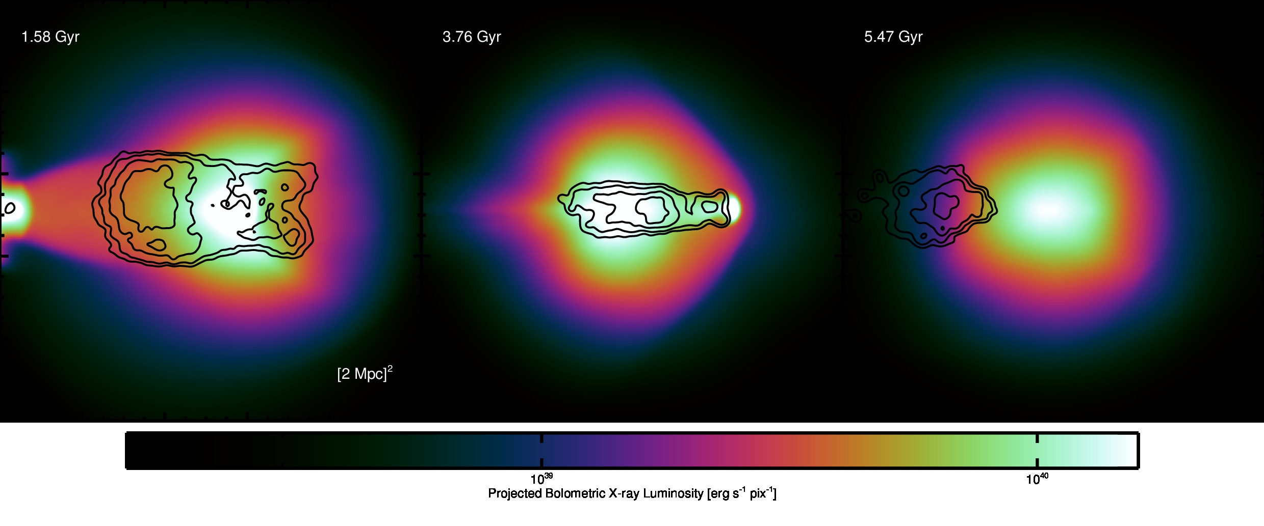
Figure 10: Bolometric X-ray emission from the system with radio synchrotron emission at 1.4 GHz overlayed as contours (Donnert et al. 2012). We show three different times: halo phase after the first (left) and second (middle) merger and off-center emission from an infalling stream (right).

We use our parallel projection routine SMAC2 to extract thermal and non-thermal synthetic observations from the system. In figure 10 we show projections of the X-ray emission at three different radio bright stages of the system.

The thermal evolution

of the system can be summarised as follows:

• Upon infall a large shock develops in front of the small cluster. This boosts the X-ray emission of the system, which peaks at the core passage (infall phase).

• As the small DM core leaves the host cluster, the X-ray luminosity declines rapidly. The small core drags a part of the ICM along (effectively displacing the gas after the first encounter), causing turbulence (reacceleration phase).

• When the DM core reaches its turn-around point the turbulence has decayed, the ICM relaxed and the cluster is radio dark (decay phase).

These merging phases are repeated two times as the DM core oscillates in the host potential. The mass of the sub-cluster successively declines and the host system is pre-disturbed. The core oscillations decay with time and the resulting emission peaks in the X-rays decline.

Due to the impact parameter, the ICM of the host cluster recieves angular momentum and an infalling stream of hot gas develops after the second core passage. This has been seen in other simulations of this kind as well (Ricker & Sarazin 2001). The system relaxes after roughly 6 Gyr.

The non-thermal emission

follows the spatial and temporal evolution of turbulence in the simulation. Shortly after the first passage of the smaller DM core a large volume filling off-center halo develops (fig. 10, left), which decays within 1 Gyr. After the second passage an elongated smaller halo centered on the peak X-ray emission of the pre-disturbed cluster can be seen (fig. 10, middle). After relaxation of the DM cores, large off-center emission develops on top of the turbulent infall stream (fig. 10, right). In between these phases the system becomes radio quiet as expected from analytical models.

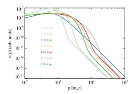
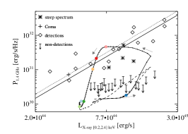
Figure 11: Left: Exemplary CRe spectrum of a particle in the simulation at different times. Middle: Observed radio-X-ray correlation (black line) and observed halos (diamonds, Coma: cross, ultra-steep: asterisks), upper limits (arrows). Simulated system (black curve, 10 Myr intervalls marked), simulated injection only (dashed curve). Colored dots correspond to the curves shown in the other panels. Right: Observed radio spectra of Coma (dots) and A521 (diamonds) and of the system at different times.

For a more quantative analysis

we will focus on the first passage only. In figure 11 (left) we show CRe electron spectra from a single particle in the simulation at seven times between 1 Gyr and 3.5 Gyrs. At 1 Gyr the CRe spectrum is in the equillibrium state between injection and cooling (blue). At 1.5 Gyr (maximum halo brightness) the spectrum shows the typical bending from turbulent reacceleration (light red). In the following times the population cools, i.e. reacceleration is not efficient anymore and CRe diffuse to synchrotron dark momenta.

In figure 11, middle panel, we show the evolution of the system in the P14-LX plane (black line). We mark every 0.2 Myr with a small dot on the line and the times shown in the other two plots with corresponding colours. The injection only model is shown as a dashed line. The observed correlation (straight black line), observed halos (diamonds) and ultra-steep spectrum halos (asterisks) and upper-limits (arrows) are added as well. In this model, the system is below the upper-limits in its initial equillibrium state (blue dot). Upon infall the shock rapidly increases X-ray and synchrotron luminosity. In the reacceleration phase the X-ray luminosity declines, because the DM core drags ICM gas out of the host system. This causes turbulence and reacceleration, which boosts the radio luminosity to maximum brightness and on the correlation (light red point). As turbulence decays the radio emission declines and the cluster leaves the correlation. Within one Gyr the radio luminosity falls below the upper limits again.

In figure 11, right panel we show synchrotron spectra of the system. The colours correspond to the times discussed before. The synchrotron spectrum at 1Gyr (dark blue) is consistent with the analytical expectation for the equillibrium of cooling and injection (eq. 4). At its maximum brightness of the system, its radio spectrum is flatter than the observed Coma spectrum. The simulated spectrum then steepens with time during the cooling phase. At 1.7 Gyr it fits the Coma spectrum (filled dots) and at 1.8 Gyr the ultra-steep spectrum of A521 (diamonds). With time the spectrum flattens again and approaches the equillibrium spectrum at 3.4 Gyrs.

5 Conclusions

We reported on the status of models for giant radio halos. Reviewing the current picture on radio halos from observations, we presented a short introduction to hadronic models. Using a pure hadronic model in a cosmological MHD simulation, we argued that hadronic models fail to simultaneously reproduce key observables:

• the Coma radio profile within the non-thermal pressure constrains,

• the Coma Compton-y - radio correlation

• the Coma spectrum and radio brightness within the current $\gamma$-ray upper limits,

• the bimodal distribution in cluster brightness.

We put forward three theoretical arguments against non-classical hadronic (streaming) models:

• Galaxy clusters are unlikely to be free of turbulence on small scales due to high Reynolds numbers and constant infall of small DM haloes.

• Efficient damping does not imply complete absense of turbulence if a cascade is present.

• Linear theory is not applicable for non-negligable damping. In turn non-linear theory predicts efficient CR scattering also for small pitch angles.

Considering this evidence we presented as short introduction to reacceleration models. We motivated the transport equation and its terms governing cooling, injection and reacceleration of the CRe population. We presented first results from a numerical approach to the problem in the framework of idealised cluster collisions. Using a constant injection of CRe, the idealised system reproduces key observables, specifically:

• the variety of observed spectral indices, from flat to ultra-steep

• the transient nature of radio halos

This reaffirms prior expectations from theoretical approaches. Naturally this idealised model is only a first step towards a more detailed modelling of the non-thermal components of the ICM. Upcoming radio telescopes like LOFAR will test our current understanding of CR dynamics and detailed numerical modelling in a cosmological framework seems highly appropriate.

We would like to emphasize that future approaches must include CR protons as well, and the absense of any clear observational signature of these particles remains an exciting problem in the next decades. One may also consider that state-of-the-art models for radio haloes require a plasma, not a fluid model of the ICM on small scales. This comes with significant complications in the physics, but bares the chance of a more complete understanding of the microphysics of the ICM, a truly unique plasma.