Higher order statistics of curvature perturbations in $IFF$ model and its Planck constraints

Abstract

We compute the power spectrum $\mathcal{P}_{\zeta}$ and non-linear parameters $f_{NL}$ and $\tau_{NL}$ of the curvature perturbation induced during inflation by the electromagnetic fields in the kinetic coupling model ($IFF$ model). By using the observational result of $\mathcal{P}_{\zeta},f_{NL}$ and $\tau_{NL}$ reported by the Planck collaboration, we study the constraint on the model comprehensively. Interestingly, if the single slow-rolling inflaton is responsible for the observed $\mathcal{P}_{\zeta}$, the constraint from $\tau_{NL}$ is most stringent. We also find a general relationship between $f_{NL}$ and $\tau_{NL}$ generated in this model. Even if $f_{NL}\sim\mathcal{O}(1)$, a detectable $\tau_{NL}$ can be produced.

1 Introduction

Recently, a possibility of a vector field playing important roles during inflation has been intensely studied. Although a U(1) gauge field is not fluctuated during inflation in its minimal form due to the conformal symmetry, several ideas to extend it are proposed. Among them, the kinetic coupling model [1] is nicely simple, free of ghost instabilities [2] and well motivated by the supergravity or the string theory frame work [3, 4, 5, 6, 7, 8]. The model action is given by

$$S_{A}=\int\mathrm{d}\eta\mathrm{d}^{3}x\sqrt{-g}\left[-\frac{1}{4}I^{2}(\phi)F_{\mu\nu}F^{\mu\nu}\right],\quad\left(F_{\mu\nu}\equiv\partial_{\mu}A_{\nu}-\partial_{\nu}A_{\mu}\right),$$ (1.1)

where $A_{\mu}$ is a gauge field, $\phi$ is a homogeneous and dynamical scalar field which is not necessarily the inflaton and $\eta$ is the conformal time. Extensive literature explores its theoretical and observational consequences.

Earlier works are aimed at generating the primordial magnetic field during inflation or “inflationary magnetogenesis” ( e.g., [9, 10] and reference therein). It is observationally known that most galaxies and galaxy clusters have $\mathcal{O}(10^{-6})$G magnetic fields and recently $\mathcal{O}(10^{-15})$G magnetic field in void regions are reported to be detected [11, 12, 13, 14]. Since no successful astrophysical mechanism which can illustrate their origins are known, it is interesting to seek them in the inflation era. Under such conditions, the kinetic coupling model was expected to realize the magnetogenesis. Unfortunately, however, it turns out that the model suffers from the so-called back reaction problem [5, 15, 16, 17] to generate the primordial magnetic field enough to explain the observations. The back reaction problem addresses that the energy density of the electromagnetic fields should be less than the inflation energy density, otherwise the consistency of inflationary magnetogenesis is invalid (see sec. 2). As another theoretical problem, so-called a strong coupling problem is also stressed [15]. This problem restricts the small kinetic coupling $I(\phi)\ll 1$ during inflation to ensure the perturbative approach in terms of quantum loop effects [4, 15]. When these problems are taken seriously, there does not exist any successful inflationary magnetogenesis scenario even in the context of the kinetic coupling model. Beyond the context of the inflationary magnetogenesis to generate the observed magnetic fields, recently, the gauge field has been focused on as a source of the adiabatic curvature perturbations and also the tensor perturbations  [20, 21, 22, 23]. It gives specific features in the perturbations, e.g., as a statistical anisotropy [28, 29, 30, 31, 32], non-gaussianity [33, 34, 35, 36, 37, 38], and cross correlations between the gauge field and the curvature/tensor perturbations  [39, 41, 40]. In other words, in a similar way to the back reaction problem, it is expected that the precise information about the primordial perturbations derived from the cosmological observations gives a new constraint on the kinetic coupling model. Quite recently, the Planck collaboration has reported updated observational information about the primordial curvature perturbations, especially, e.g., the amplitude of curvature perturbation $\mathcal{P}_{\zeta}$, non-linearity parameters $f_{\rm NL}$ and $\tau_{\rm NL}$ which represent the amplitudes of the bispectrum and trispectrum respectively [44, 45]. Thus it is appropriate time to investigate the primordial curvature perturbations induced from the gauge field in the kinetic coupling model precisely, and to derive a constraint on the model.

In spite of its importance, limited attentions are paid to induced curvature perturbations in the kinetic coupling model. Actually previous works are done only under either of following assumptions ; (1) $I(\phi)\propto a^{\pm 2}$ is given and it produces exact scale-invariant spectra of electric or magnetic fields. (2) $\phi$ of $I(\phi)$ is the inflaton field, where the quantum fluctuations of the inflaton is responsible for the dominant source of the curvature perturbations and the effect of the gauge field on the inflaton fluctuations through the direct coupling $I(\phi)F_{\mu\nu}F_{\mu\nu}$ is investigated.

In this paper, we consider more general situations, where we specify neither the scalar field in the kinetic coupling, $I$, nor the dominant source of the curvature perturbations and the functional form of $I$ is given by $I\propto a^{-n}$ for an arbitrary $n\geq 2$. Our strategy is simple. We derive the evolution equation of $\zeta$ in the presence of electromagnetic fields and calculate its power spectrum $\mathcal{P}_{\zeta}$ and non-gaussianities ($f_{\rm NL},\tau_{\rm NL})$ induced by electromagnetic field in the kinetic coupling model with $I(\phi)\propto a^{-n}$. Then, by using observation result of Planck collaboration [44, 45], we obtain the constraints on the parameters of the model and inflation, which are not only the tilt of electromagnetic fields spectrum corresponding to the model parameter, $n$, but also inflation energy scale and total e-folding number. As a result, we find that the allowed parameter region is reduced from the one where only the back reaction problem is taken into account. Interestingly, the constraint from $\tau_{\rm NL}$ is most stringent under the assumption that the dominant source of the curvature perturbations is attributed to the quantum fluctuations of the inflaton field. We also find that in the kinetic coupling model the large $\tau_{\rm NL}\ (\gtrsim 10^{3})$ can be realized even for the small $f_{\rm NL}\ (\lesssim 10)$.

The rest of paper is organized as follows. In section 2, we review the kinetic coupling model and discuss the back reaction problem. In section 3, we derive the evolution equation of $\zeta$ induced by the electromagnetic field during inflation. We also calculate its correlators up to 4-point and obtain induced $\mathcal{P}_{\zeta},f_{\rm NL}$ and $\tau_{\rm NL}$. In section 4, we compare these quantities to observational results and show the restricted parameter region. We conclude in section 5.

2 Review of the kinetic coupling model and the back reaction problem

2.1 Model set up

We consider the kinetic coupling model [1, 2, 5, 3, 4, 6, 7, 8] in this paper. Although it can not generate the primordial magnetic field which is strong enough to be more than $10^{-15}$G at present [15, 16, 17], it is nicely simple and gives us the essential understanding of the problem. Moreover this model is interesting in terms of CMB observations because it can produce detectable level of non-gaussianities. In this section we review the model.

In the kinetic coupling model, the kinetic term of U(1) gauge field is modified as $F_{\mu\nu}F^{\mu\nu}\rightarrow I^{2}(\phi)F_{\mu\nu}F^{\mu\nu}$ where $\phi$ is a homogeneous scalar field and is not necessarily inflaton and $I(\phi)$ is phenomenologically assumed to be the power function of conformal time, $I\propto\eta^{n}$. To restore the Maxwell theory after inflation, $I$ is required to be unity at the end of inflation $\eta_{\rm f}$. Thus $I(\phi)$ is reduced as

$$I(\phi)=\left\{\begin{array}[]{cc}(\eta/\eta_{\rm f})^{n}&(\eta<\eta_{\rm f})\\ 1&(\eta\geq\eta_{\rm f})\end{array}\,.\right.$$ (2.1)

We do not specify the Lagrangian of $\phi$ and assume the quasi de Sitter inflation, the Einstein gravity and the flat FLRW metric. Note that hereafter we consider only positive $n$ to avoid the strong coupling problem. Because if $n$ is negative and the QED coupling $e\bar{\psi}\gamma^{\mu}\psi A_{\mu}$ exists, its effective coupling constant, $e/I$, becomes much larger than unity during inflation. In that case, we can not calculate the behavior of $A_{\mu}$ without fully taking account of the interaction effects [15].

Let us take the radiation gauge, $A_{0}=\partial_{i}A_{i}=0$, and expand the transverse part of $A_{i}$ with the polarization vector $\epsilon_{i}^{(\lambda)}$ and the creation/annihilation operator $a^{\dagger(\lambda)}_{\bm{k}}/a^{(\lambda)}_{\bm{k}}$ as

$$A_{i}(\eta,\bm{x})=\sum_{\lambda=1}^{2}\int\frac{{\rm d}^{3}k}{(2\pi)^{3}}e^{i\bm{k\cdot x}}\epsilon_{i}^{(\lambda)}(\hat{\bm{k}})\left[a_{\bm{k}}^{(\lambda)}\mathcal{A}_{k}(\eta)+a_{-\bm{k}}^{{\dagger}(\lambda)}\mathcal{A}_{k}^{*}(\eta)\right]\,,$$ (2.2)

where the hat of $\hat{\bm{k}}$ denotes the unit vector and $(\lambda)$ is the polarization label. Notice the behavior of $\mathcal{A}_{k}$ does not depend on the polarization in this model. The equation of motion during inflation is given by

$$\left[\partial_{\eta}^{2}+k^{2}-\frac{n(n-1)}{\eta^{2}}\right](I\mathcal{A}_{k})=0\,.$$ (2.3)

Assuming the Bunch-Davies vacuum, $I\mathcal{A}_{k}=(2k)^{-1/2}e^{ik\eta}$, in the sub-horizon limit, the asymptotic solution of eq. (2.3) in the super-horizon is

$$|I\mathcal{A}_{k}(\eta)|=\frac{\Gamma(n-1/2)}{\sqrt{2\pi k}}\left(\frac{-k\eta}{2}\right)^{1-n},\quad\left(-k\eta\ll 1,\ n>\frac{1}{2}\right),$$ (2.4)

where we have neglected the constant phase factor. For $0<n<1/2$, the asymptotic solution is different and the generated electromagnetic fields are weaker than the cases of $n>1/2$. Hence we focus on $n>1/2$ hereafter.

At this point, we can acquire three important consequences in this model. First, the generated magnetic field is negligible compared with the electric field. The power spectrum of electric and magnetic fields are given by

$$\mathcal{P}_{E}(\eta,k)\equiv\frac{k^{3}|\partial_{\eta}\mathcal{A}_{k}|^{2}}{\pi^{2}a^{4}},\qquad\mathcal{P}_{B}(\eta,k)\equiv\frac{k^{5}|\mathcal{A}_{k}|^{2}}{\pi^{2}a^{4}},$$ (2.5)

where two polarization modes are already summed. Then $\mathcal{P}_{B}/\mathcal{P}_{E}\simeq(-k\eta)^{2}$ and the magnetic field is much smaller than the electric field in the super-horizon. Second, the unique model parameter $n$ controls both the time dependence and the tilt of the electromagnetic energy spectrum. The energy contribution from each $\ln k$ mode of electric and magnetic fields can be calculated from the action eq. (1.1) ,

$$\frac{\mathrm{d}\rho_{E}}{\mathrm{d}\ln k}=\frac{1}{2}I^{2}\mathcal{P}_{E}(\eta,k)=\frac{\Gamma^{2}(n+\frac{1}{2})}{2^{2-2n}\pi^{3}}H^{4}\left(-k\eta\right)^{2(2-n)},$$ (2.6)

$$\frac{\mathrm{d}\rho_{B}}{\mathrm{d}\ln k}=\frac{1}{2}I^{2}\mathcal{P}_{B}(\eta,k)=\frac{\Gamma^{2}(n-\frac{1}{2})}{2^{4-2n}\pi^{3}}H^{4}\left(-k\eta\right)^{2(3-n)},$$

where $H$ is Hubble parameter. The above equation tells that the electric field grows (decays) and the spectrum of the electric energy density is red-tilted (blue-tilted) for $n>2$ ($n<2$). The flat spectrum can be realized in $n=2$ case where the electric field stays constant. In the magnetic case, the border of $n$ is 3 in stead of 2. Finally, the magnetic power spectrum at present is

$$\mathcal{P}^{1/2}_{B}(\eta_{\rm now},k)=\frac{\Gamma(n-\frac{1}{2})}{2^{\frac{3}{2}-n}\pi^{\frac{3}{2}}}(a_{\rm f}H)^{n-1}k^{3-n}\sim 10^{23n-80}{\rm G}\times\left(\frac{\rho_{\rm inf}^{1/4}}{10^{16}{\rm GeV}}\right)^{n-1}\left(\frac{k}{1{\rm Mpc}^{-1}}\right)^{3-n},$$ (2.7)

where $\rho_{\rm inf}$ is the energy density of the inflaton and $a_{\rm f}$ is a scale factor at the end of inflation ($a=1$ at the present). Here we assume the instant reheating and have $a_{\rm f}=\rho_{\gamma}/\rho_{\rm inf}$ with $\rho_{\gamma}$ being the present energy density of the radiation which is given by $\rho_{\gamma}\approx 5.7\times 10^{-125}M_{\rm Pl}^{4}$. From the above expression, we find that $n\gtrsim 3$ is required to make the cosmic magnetic field whose strength is more than the observational lower bound from blazars, $10^{-15}$G, at Mpc scale.

2.2 back reaction problem

In sec. 2.1, we assume that inflation continues and the electromagnetic generation does not change regardless of the amount of the electromagnetic fields. But if the energy density of the electromagnetic field $\rho_{\rm em}$ becomes comparable with that of inflaton, inflation itself or the generation of electromagnetic fields must be altered. Thus for the consistency of the above calculation, $\rho_{\rm em}<\rho_{\rm inf}$ should be satisfied. Unfortunately, however, in the parameter range where the generated magnetic field is enough strong to explain the blazar observation, namely $n\gtrsim 3$, $\rho_{\rm em}$ becomes larger than $\rho_{\rm inf}$. This problem is called “back reaction problem” .

From eq. (2.4), the energy density of electromagnetic field during inflation is given by

$$\rho_{\rm em}(\eta)\simeq\frac{I^{2}}{2}\int^{aH}_{k_{\rm min}}\frac{\mathrm{d}k}{k}\mathcal{P}_{E}(\eta,k)=\frac{\Gamma^{2}(n+\frac{1}{2})}{2^{2-2n}\pi^{3}}H^{4}\left[\frac{\left(-k_{\rm min}\eta\right)^{2(2-n)}-1}{2n-4}\right]\,,$$ (2.8)

where we ignore the contribution of $\mathcal{P}_{B}$ and $k_{\rm min}$ is the wave number of the mode which crosses the horizon when $I(\eta)$ starts to behave as $(\eta/\eta_{\rm f})^{n}$. Because of $-k_{\rm min}\eta<1$, $\rho_{\rm em}(\eta)$ is an increasing function of $\eta$ for $n\geq 2$ while the $\eta$ dependence is negligible for $n<2$. Thus for $n\geq 2$, it is sufficient to require $\rho_{\rm inf}>\rho_{\rm em}(\eta)$ at the end of inflation for its satisfaction over the entire period of inflation. This condition puts the upper limit on $\rho_{\rm inf}$,

$$\frac{\rho_{\rm inf}}{M_{\rm Pl}^{4}}\,<\,\frac{2^{2-2n}3^{2}\pi^{3}}{\Gamma^{2}(n+\frac{1}{2})}D_{n}^{-1}(N_{\rm tot})\qquad(n\geq 2),$$ (2.9)

where $N_{\rm tot}\equiv-\ln\left|k_{\rm min}\eta_{\rm f}\right|$ and we define new function $D_{n}$ for later simplicity,

$$D_{n}(X)\equiv\frac{e^{(2n-4)X}-1}{2n-4},\qquad\lim_{n\rightarrow 2}D_{n}(X)=X\,.$$ (2.10)

Substituting eq. (2.9) into eq. (2.7), one can obtain the upper limit of the magnetic power spectrum at present. For example, the upper limits for $n=3$ are

$$\mathcal{P}^{1/2}_{B}(\eta_{\rm now},k,n=3)<1.8\times 10^{-28}{\rm G}\times\exp\left[50-N_{\rm tot}\right].$$ (2.11)

For $n>3$, the upper bound on $\mathcal{P}_{B}(\eta_{\rm now},k)$ is more stringent. Therefore the kinetic coupling model can not generate the primordial magnetic field with sufficient strength because of the back reaction problem.

3 Curvature perturbation induced by electromagnetic fields

Recently the effect of vector fields in the kinetic coupling model on the curvature perturbation draws attention. The electromagnetic fields behave as isocurvature perturbations and they can source the adiabatic curvature perturbation on super-Hubble scales. The induced curvature perturbation has distinguishing non-gaussianities which can be large enough for detection [36, 37]. Planck data released in this March has given precise information about the primordial curvature perturbation and also tighter constraints on the non-linearity parameters which parameterize the non-Gaussian features of the primordial curvature perturbation. These Planck constraints can translate into the limits on the parameters of the kinetic coupling model and inflation. In this section, we derive the curvature perturbation induced by the electromagnetic fields in the kinetic coupling model during inflation. Then we compute its two-point, three-point, four-point correlators and their related non-linearity parameters.

3.1 Evolution equation of $\zeta_{\rm em}$

The curvature perturbation $\zeta(t,\bm{x})$ is defined as the perturbation of the scale factor $a(t,\bm{x})$ on the uniform density slice, $\zeta(t,\bm{x})\equiv\ln\left[a(t,\bm{x})/a(t)\right]$ where $t$ is the cosmic time. Let us derive the evolution equation of $\zeta(t,\bm{x})$. The energy continuity equation holds on super-Hubble scales [43],

$$\dot{\rho}(t) =-3\frac{\dot{a}(t,\bm{x})}{a(t,\bm{x})}[\rho(t)+p(t,\bm{x})]$$

$$=-3\left(H(t)+\dot{\zeta}(t,\bm{x})\right)\left[\rho(t)+p(t)+\delta p_{\rm nad}(t,\bm{x})\right].$$ (3.1)

By subtracting its homogeneous part, we obtain the evolution equation of the curvature perturbation on super-Hubble scales,

$$\dot{\zeta}(t,\bm{x})=-\frac{H(t)\delta p_{\rm nad}(t,\bm{x})}{\rho(t)+p(t)}\,.$$ (3.2)

Here the non-adiabatic pressure is defined as $\delta p_{\rm nad}(t,\bm{x})\equiv\delta p(t,\bm{x})-\frac{\dot{p}(t)}{\dot{\rho}(t)}\delta\rho(t,\bm{x}).$ In our case where the background energy density is dominated by the inflaton field and the energy density of the electromagnetic field is treated as a perturbation, we have

$$p_{\rm inf}\simeq-\left(1-\frac{2}{3}\epsilon\right)\rho_{\rm inf},\quad\delta\rho_{\rm em}=3\delta p_{\rm em},$$ (3.3)

where $\epsilon$ is the slow-roll parameter and indices “inf” and “em” denote the contribution from inflaton and electromagnetic fields, respectively. Hence eq. (3.2) reads [25, 27],

$$\dot{\zeta}^{\rm em}(t,\bm{x})=-\frac{2H(t)}{\epsilon\rho_{\rm inf}}\delta\rho_{\rm em}(t,\bm{x}),$$ (3.4)

in the leading order of $\epsilon$. Integrating it, we finally obtain the expression of curvature perturbation induced by electromagnetic fields as [20]

$$\zeta^{\rm em}(t,\bm{x})=-\frac{2H}{\epsilon\rho_{\rm inf}}\int^{t}_{t_{0}}dt^{\prime}\delta\rho_{\rm em}(t^{\prime},\bm{x}),$$ (3.5)

where $H,\epsilon$ and $\rho_{\rm inf}$ are assumed to be constant during inflation and $t_{0}$ denotes an initial time when $\zeta^{\rm em}(t_{0},\bm{x})=0$. Let us assume that the electromagnetic fields are originally absent before the generation during inflation and thus all electromagnetic fields exist as perturbations, and hence we have $\delta\rho_{\rm E}=\rho_{\rm E}=\frac{1}{2}I^{2}(\eta)\bm{E}^{2}(\eta,\bm{x})$ and neglect the contribution of the magnetic energy (see the discussion below eq. (2.5)). By performing Fourier transformation of $\bm{E}(\eta,\bm{x})$, the electromagnetic energy density is written in the convolution of two Fourier transformed electric fields as

$$\delta\rho_{\rm em}(\eta,\bm{k})\simeq\frac{1}{2}I^{2}(\eta)\iint\frac{\mathrm{d}^{3}p\,\mathrm{d}^{3}q}{(2\pi)^{3}}\delta(\bm{p}+\bm{q}-\bm{k})\bm{E}(\eta,\bm{p})\cdot\bm{E}(\eta,\bm{q})\,.$$ (3.6)

By using eq. (2.2), (2.4), (3.6) and the definition of the electric field, $E_{i}\equiv a^{-2}\partial_{\eta}A_{i}$, eq. (3.5) reads

$$\zeta^{\rm em}(\eta,\bm{k})=\frac{c^{2}_{n}\rho_{\rm inf}}{9\epsilon M_{\rm Pl}^{4}}\iint^{k_{\rm max}}_{k_{\rm min}}\frac{\mathrm{d}^{3}p\,\mathrm{d}^{3}q}{(2\pi)^{3}}\,\delta(\bm{p}+\bm{q}-\bm{k})\,p^{\frac{1}{2}-n}q^{\frac{1}{2}-n}\\ \times\sum_{\lambda,\sigma}\epsilon^{(\lambda)}_{i}(\hat{\bm{p}})\,\epsilon^{(\sigma)}_{i}(\hat{\bm{q}})\,\left(a^{(\lambda)}_{\bm{p}}+a^{\dagger(\lambda)}_{\bm{-p}}\right)\left(a^{(\sigma)}_{\bm{q}}+a^{\dagger(\sigma)}_{\bm{-q}}\right)\int^{\eta}_{\eta_{0}}\mathrm{d}\tilde{\eta}\,\tilde{\eta}^{3-2n}$$ (3.7)

where the lower end of the time integration, $\eta_{0}=-{\rm max}[p,q]^{-1}$, represents that only super-horizon modes are considered as physical modes, $k_{\rm max}=-\eta_{\rm f}^{-1}$ is the maximum wave number exiting the horizon during inflation and we define $c_{n}$ as

$$I\partial_{\eta}A_{k}(\eta)=c_{n}\,k^{\frac{1}{2}-n}\eta^{-n},\quad c_{n}\equiv\frac{2^{n}\Gamma(n+\frac{1}{2})}{\sqrt{2\pi}}\,.$$ (3.8)

Before closing this subsection, let us note that the anisotropic stress which can also source the curvature perturbation is not taken into account here. However, the contribution from the electromagnetic anisotropic stress is suppressed by slow-roll parameter $\epsilon$ in comparison to the contribution from the non-adiabatic pressure during inflation [20]. Thus eq. (3.5) is the leading order equation.

3.2 Calculation of 2, 3, 4-point correlators

Let us calculate two, three and four-point correlation function of the curvature perturbation in the Fourier space. At first, we consider m-point correlator,

$$\left\langle\prod_{i=1}^{m}\zeta^{\rm em}(\eta,\bm{k}_{i})\right\rangle=\left\langle\prod_{i=1}^{m}\left(\frac{c^{2}_{n}\rho_{\rm inf}}{9\epsilon M_{\rm Pl}^{4}}\right)\iint^{k_{\rm max}}_{k_{\rm min}}\frac{\mathrm{d}^{3}p_{i}\,\mathrm{d}^{3}q_{i}}{(2\pi)^{3}}\delta(\bm{p}_{i}+\bm{q}_{i}-\bm{k}_{i})p_{i}^{\frac{1}{2}-n}q_{i}^{\frac{1}{2}-n}\right.\\ \left.\times\sum_{\lambda_{i},\sigma_{i}}\epsilon^{(\lambda_{i})}_{j_{i}}(\hat{\bm{p}_{i}})\epsilon^{(\sigma_{i})}_{j_{i}}(\hat{\bm{q}_{i}})\left(a^{(\lambda_{i})}_{\bm{p}_{i}}+a^{\dagger(\lambda_{i})}_{\bm{-p}_{i}}\right)\left(a^{(\sigma_{i})}_{\bm{q}_{i}}+a^{\dagger(\sigma_{i})}_{\bm{-q}_{i}}\right)\int^{\eta}_{\eta_{0,i}}\mathrm{d}\tilde{\eta}_{i}\,\tilde{\eta}_{i}^{3-2n}\right\rangle\,,$$ (3.9)

where the bracket $\langle\cdots\rangle$ denotes the vacuum expectation value and is only relevant to $a_{\bm{k}}^{(\lambda)}$ and $a_{-\bm{k}}^{\dagger(\lambda)}$. One can show $\left\langle m{\rm-point}\right\rangle\equiv\left\langle\prod_{i=1}^{m}\left(a^{(\lambda_{i})}_{\bm{p}_{i}}+a^{\dagger(\lambda_{i})}_{\bm{-p}_{i}}\right)\left(a^{(\sigma_{i})}_{\bm{q}_{i}}+a^{\dagger(\sigma_{i})}_{\bm{-q}_{i}}\right)\right\rangle$ is given by

$$\left\langle 2{\rm-point}\right\rangle=2(2\pi)^{6}\delta(\bm{p}_{1}+\bm{q}_{2})\delta(\bm{p}_{2}+\bm{q}_{1})\delta^{\lambda_{1}\sigma_{2}}\delta^{\lambda_{2}\sigma_{1}}\,,$$ (3.10)

$$\left\langle 3{\rm-point}\right\rangle=8(2\pi)^{9}\delta(\bm{p}_{1}+\bm{q}_{2})\delta(\bm{p}_{2}+\bm{q}_{3})\delta(\bm{p}_{3}+\bm{q}_{1})\delta^{\lambda_{1}\sigma_{2}}\delta^{\lambda_{2}\sigma_{3}}\delta^{\lambda_{3}\sigma_{1}}\,,$$ (3.11)

$$\left\langle 4{\rm-point}\right\rangle=16\left\{(2\pi)^{12}\delta(\bm{p}_{1}+\bm{q}_{2})\delta(\bm{p}_{2}+\bm{q}_{3})\delta(\bm{p}_{3}+\bm{q}_{4})\delta(\bm{p}_{4}+\bm{q}_{1})\delta^{\lambda_{1}\sigma_{2}}\delta^{\lambda_{2}\sigma_{3}}\delta^{\lambda_{3}\sigma_{4}}\delta^{\lambda_{4}\sigma_{1}}\right.$$

$$\qquad\qquad\qquad\quad\left.+(2\leftrightarrow 3)+(3\leftrightarrow 4)\Big{\}}+({\rm disconnected\ terms})\right.\,,$$ (3.12)

Since the calculation processes for $m=$2, 3 and 4 are analogous, we illustrate only the $m=2$ case in detail. By virtue of the delta function and the Kronecker delta in eq. (3.10), the polarization factor in eq. (3.9) reads

$$\sum_{\lambda_{1},\lambda_{2}}\epsilon^{(\lambda_{1})}_{j_{1}}(\hat{\bm{p}_{1}})\epsilon^{(\lambda_{2})}_{j_{1}}(-\hat{\bm{p}_{2}})\epsilon^{(\lambda_{2})}_{j_{2}}(\hat{\bm{p}_{2}})\epsilon^{(\lambda_{1})}_{j_{2}}(-\hat{\bm{p}_{1}})=\Bigl{(}\delta_{j_{1}j_{2}}-(\hat{\bm{p}}_{1})_{j_{1}}(\hat{\bm{p}}_{1})_{j_{2}}\Bigr{)}\Bigl{(}\delta_{j_{1}j_{2}}-(\hat{\bm{p}}_{2})_{j_{1}}(\hat{\bm{p}}_{2})_{j_{2}}\Bigr{)}\,.$$ (3.13)

and the $\tilde{\eta}$ integral in eq. (3.9) reads

$$\prod_{i=1}^{2}\int^{\eta}_{\eta_{0}}\mathrm{d}\tilde{\eta}_{i}\,\tilde{\eta}_{i}^{3-2n}=\left[\frac{\eta^{4-2n}-(-{\rm max}[p_{1},p_{2}])^{2n-4}}{2n-4}\right]^{2}\,.$$ (3.14)

Next one can perform the $q_{i}$ integrals by using $\delta(\bm{p}_{i}+\bm{q}_{i+1})$. In the $m=2$ case, we obtain

$$\left\langle\zeta^{\rm em}_{\bm{k}_{1}}\zeta^{\rm em}_{\bm{k}_{2}}(\eta)\right\rangle=2\delta(\bm{k}_{1}+\bm{k}_{2})\left(\frac{c^{2}_{n}\rho_{\rm inf}}{9\epsilon M_{\rm Pl}^{4}}\right)^{2}\iint^{k_{\rm max}}_{k_{\rm min}}\mathrm{d}^{3}p_{1}\mathrm{d}^{3}p_{2}\delta(\bm{p}_{2}-\bm{p}_{1}-\bm{k}_{2})\,p_{1}^{1-2n}p_{2}^{1-2n}\\ \times\Bigl{(}\delta_{j_{1}j_{2}}-(\hat{\bm{p}}_{1})_{j_{1}}(\hat{\bm{p}}_{1})_{j_{2}}\Bigr{)}\Bigl{(}\delta_{j_{1}j_{2}}-(\hat{\bm{p}}_{2})_{j_{1}}(\hat{\bm{p}}_{2})_{j_{2}}\Bigr{)}\left[\frac{\eta^{4-2n}-(-{\rm max}[p_{1},p_{2}])^{2n-4}}{2n-4}\right]^{2}\,.$$ (3.15)

If $n\geq 2$, the biggest contributions of the integrals in eq. (3.15) come from the pole where $p_{1}\simeq k_{\rm min}$ and $p_{2}\simeq k_{\rm min}$. In the rest of this paper, we concentrate on the cases where $n\geq 2$. Then eq. (3.15) can be evaluated by the pole contributions. Note the integrand has the symmetry of $\bm{p}_{1}\leftrightarrow\bm{p}_{2}$. Even in the case of $m=3$ and 4, the cyclic symmetry like, $\bm{p}_{1}\rightarrow\bm{p}_{2}\rightarrow\cdots\rightarrow\bm{p}_{m}\rightarrow\bm{p}_{1}$, exists. Thus if the $p_{1}$ pole is evaluated, the other contributions can be easily duplicated. The $p_{1}$ pole contribution in eq. (3.15) is evaluated as

$$\left\langle\zeta^{\rm em}_{\bm{k}_{1}}\zeta^{\rm em}_{\bm{k}_{2}}(\eta)\right\rangle\big{|}_{p_{1}\simeq k_{\rm min}}=\frac{32\pi}{3\,k_{1}^{3}}\delta(\bm{k}_{1}+\bm{k}_{2})\left(\frac{c^{2}_{n}\rho_{\rm inf}}{9\epsilon M_{\rm Pl}^{4}}\right)^{2}\left[\frac{(k_{1}/k_{\rm min})^{2n-4}-1}{2n-4}\right]\left[\frac{(-k_{1}\eta)^{4-2n}-1}{2n-4}\right]^{2},$$ (3.16)

where we use the angular integral, $\int\mathrm{d}\Omega_{k}\hat{\bm{k}}_{i}\hat{\bm{k}}_{j}=\frac{4\pi}{3}\delta_{ij}$, and assume $k_{1}=k_{2}\gg k_{\rm min}$. Notice additional factors like $({\rm max}[k_{1},k_{3}]/{\rm min}[k_{1},k_{3}])^{2n-4}\geq 1$ appear in the case of $m=3$ and 4. Nevertheless, we conservatively ignore those factors for simplicity by assuming all reference wave numbers are close to the CMB scale, $k_{i}\sim k_{\rm CMB}$. Except for this point, the calculations of $m=3,4$ case are closely analogous to $m=2$ case. Therefore we obtain 2, 3 and 4-point connected correlation function of the electromagnetic induced curvature perturbation at the end of inflation $\eta_{\rm f}$ as

$$\left\langle\zeta^{\rm em}_{\bm{k}_{1}}\zeta^{\rm em}_{\bm{k}_{2}}(\eta_{\rm f})\right\rangle =\frac{64\pi}{3k_{1}^{3}}\delta(\bm{k}_{1}+\bm{k}_{2})\left(\frac{c^{2}_{n}\rho_{\rm inf}}{9\epsilon M_{\rm Pl}^{4}}\right)^{2}D_{n}(N_{\rm tot}-N_{\rm CMB})D_{n}(N_{\rm CMB})^{2},$$ (3.17)

$$\left\langle\zeta^{\rm em}_{\bm{k}_{1}}\zeta^{\rm em}_{\bm{k}_{2}}\zeta^{\rm em}_{\bm{k}_{3}}(\eta_{\rm f})\right\rangle =\frac{64\pi}{3}\delta(\bm{k}_{1}+\bm{k}_{2}+\bm{k}_{3})\left(\frac{c^{2}_{n}\rho_{\rm inf}}{9\epsilon M_{\rm Pl}^{4}}\right)^{3}D_{n}(N_{\rm tot}-N_{\rm CMB})D_{n}(N_{\rm CMB})^{3}$$

$$\qquad\times\left[\frac{1+(\hat{\bm{k}}_{1}\cdot\hat{\bm{k}}_{2})^{2}}{(k_{1}k_{2})^{3}}+2\ {\rm perms}\right],$$ (3.18)

$$\left\langle\zeta^{\rm em}_{\bm{k}_{1}}\zeta^{\rm em}_{\bm{k}_{2}}\zeta^{\rm em}_{\bm{k}_{3}}\zeta^{\rm em}_{\bm{k}_{4}}(\eta_{\rm f})\right\rangle =\frac{128\pi}{3}\delta(\bm{k}_{1}+\bm{k}_{2}+\bm{k}_{3}+\bm{k}_{4})\left(\frac{c^{2}_{n}\rho_{\rm inf}}{9\epsilon M_{\rm Pl}^{4}}\right)^{4}D_{n}(N_{\rm tot}-N_{\rm CMB})D_{n}(N_{\rm CMB})^{4}$$

$$\times\left[\frac{(\hat{\bm{k}}_{1}\cdot\hat{\bm{k}}_{2})^{2}+(\hat{\bm{k}}_{1}\cdot\hat{\bm{k}}_{13})^{2}+(\hat{\bm{k}}_{2}\cdot\hat{\bm{k}}_{13})^{2}-(\hat{\bm{k}}_{1}\cdot\hat{\bm{k}}_{2})(\hat{\bm{k}}_{1}\cdot\hat{\bm{k}}_{13})(\hat{\bm{k}}_{2}\cdot\hat{\bm{k}}_{13})}{(k_{1}k_{2}k_{13})^{3}}+11\ {\rm perms}\right],$$ (3.19)

where $\bm{k}_{13}\equiv\bm{k}_{1}+\bm{k}_{3}\,,D_{n}(X)\equiv(e^{(2n-4)X}-1)/(2n-4)\,,e^{-N_{\rm CMB}}=-k_{\rm CMB}\eta_{\rm f}\,$ and $e^{N_{\rm tot}-N_{\rm CMB}}=k_{\rm CMB}/k_{\rm min}\,.$ In the limit of $n\rightarrow 2$, these results coincide with the previous works [36, 37].

When $n<2$, the correlators of induced $\zeta$ can not be computed as above because there is no pole. Then we have to calculate the correlators by brute force. But if $n$ is not too close to 2, the results are expected to depend on neither $N_{\rm tot}$ nor $N_{\rm CMB}$. It is because the source of curvature perturbation, $I^{2}\mathcal{P}_{E}(\eta,k)$, drops in the super-horizon as $\eta^{2(2-n)}$ and thus it sources $\zeta$ right after its horizon-crossing only. Therefore since the resultant correlators are not just much weaker than those in $n\geq 2$ case but depend on neither $N_{\rm tot}$ nor $N_{\rm CMB}$, the motivation to constrain them is inadequate. In this paper, we concentrate on the cases where $n\geq 2$.

3.3 Power spectrum and Non-gaussianities

Let us connect 2,3,4-point correlators to the observable quantities in order to compare them with the CMB observation results. Here relevant observable quantities are the power spectrum of the primordial curvature perturbations $\mathcal{P}_{\zeta}$, and local-type non-linearity parameters $f_{\rm NL}^{\rm local}$ and $\tau_{\rm NL}$ which parameterize the amplitudes of the 3- and 4-point functions of the curvature perturbations in Fourier space, respectively. These are defined as

$$\left\langle\zeta_{\bm{k}_{1}}\zeta_{\bm{k}_{2}}\right\rangle =(2\pi)^{3}\delta(\bm{k}_{1}+\bm{k}_{2})\frac{2\pi^{2}}{k_{1}^{3}}\mathcal{P}_{\zeta}\,,$$ (3.20)

$$\left\langle\zeta_{\bm{k}_{1}}\zeta_{\bm{k}_{2}}\zeta_{\bm{k}_{3}}\right\rangle =(2\pi)^{3}\delta(\bm{k}_{1}+\bm{k}_{2}+\bm{k}_{3})\,(2\pi^{2}\,\mathcal{P}_{\zeta})^{2}\ \frac{6}{5}\,f_{\rm NL}^{\rm local}\,\frac{\sum_{i=1}^{3}k_{i}^{3}}{\prod_{i=1}^{3}k_{i}^{3}}\,,$$ (3.21)

$$\left\langle\zeta_{\bm{k}_{1}}\zeta_{\bm{k}_{2}}\zeta_{\bm{k}_{3}}\zeta_{\bm{k}_{4}}\right\rangle =(2\pi)^{3}\delta(\bm{k}_{1}+\bm{k}_{2}+\bm{k}_{3}+\bm{k}_{4})\,(2\pi^{2}\mathcal{P}_{\zeta})^{3}\,\tau_{\rm NL}$$

$$\hskip 113.81102pt\times\left[\frac{1}{(k_{1}k_{2}k_{13})^{3}}+11\ {\rm perms}\right],$$ (3.22)

where the small deviation from scale invariant spectrum of $\mathcal{P}_{\zeta}$ is neglected. By substituting eq. (3.17) into eq. (3.20), one can easily obtain the induced power spectrum as

$$\mathcal{P}_{\zeta}^{\rm em}(k,\eta_{\rm f})=\frac{4}{3}\left(\frac{c^{2}_{n}\rho_{\rm inf}}{9\pi^{2}\epsilon M_{\rm Pl}^{4}}\right)^{2}D_{n}(N_{\rm tot}-N_{\rm CMB})D_{n}^{2}(N_{\rm CMB}).$$ (3.23)

As for $f_{\rm NL}^{\rm local}$ and $\tau_{\rm NL}$, however, $k_{i}$ dependence of eq. (3.18) and (3.19) is different from that of eq. (3.21) and (3.22), respectively. Thus they can not be compared straightforwardly .

But when eq. (3.18) and (3.19) are averaged over the direction of $\hat{\bm{k}}_{i}$, their $k_{i}$ dependence accord with that of eq. (3.21) and (3.22), respectively. After angular averaged, eq. (3.18) and (3.19) read

$$\left\langle\zeta^{\rm em}_{\bm{k}_{1}}\zeta^{\rm em}_{\bm{k}_{2}}\zeta^{\rm em}_{\bm{k}_{3}}(\eta_{\rm f})\right\rangle_{\rm ave}=\frac{2^{8}\pi}{3^{2}}\delta(\bm{k}_{1}+\bm{k}_{2}+\bm{k}_{3})\left(\frac{c^{2}_{n}\rho_{\rm inf}}{9\epsilon M_{\rm Pl}^{4}}\right)^{3}D_{n}(N_{\rm tot}-N_{\rm CMB})D_{n}^{3}(N_{\rm CMB})\frac{\sum_{i=1}^{3}k_{i}^{3}}{\prod_{i=1}^{3}k_{i}^{3}}$$ (3.24)

$$\left\langle\zeta^{\rm em}_{\bm{k}_{1}}\zeta^{\rm em}_{\bm{k}_{2}}\zeta^{\rm em}_{\bm{k}_{3}}\zeta^{\rm em}_{\bm{k}_{4}}(\eta_{\rm f})\right\rangle_{\rm ave}=\frac{2^{7}\pi}{3}\delta(\bm{k}_{1}+\bm{k}_{2}+\bm{k}_{3}+\bm{k}_{4})\left(\frac{c^{2}_{n}\rho_{\rm inf}}{9\epsilon M_{\rm Pl}^{4}}\right)^{4}D_{n}(N_{\rm tot}-N_{\rm CMB})D_{n}^{4}(N_{\rm CMB})$$

$$\times\left[\frac{1}{(k_{1}k_{2}k_{13})^{3}}+11\ {\rm perms}\right].$$ (3.25)

Therefore we obtain electromagnetic induced local-type non-gaussianities

$$f_{\rm NL}^{\rm em}=\frac{2^{2}5}{3^{3}}\left(\frac{c^{2}_{n}\rho_{\rm inf}}{9\pi^{2}\epsilon M_{\rm Pl}^{4}}\right)^{3}\mathcal{P}_{\zeta}^{-2}\,D_{n}(N_{\rm tot}-N_{\rm CMB})D_{n}^{3}(N_{\rm CMB}),$$ (3.26)

$$\tau_{\rm NL}^{\rm em}=\frac{2}{3}\left(\frac{c^{2}_{n}\rho_{\rm inf}}{9\pi^{2}\epsilon M_{\rm Pl}^{4}}\right)^{4}\mathcal{P}_{\zeta}^{-3}\,D_{n}(N_{\rm tot}-N_{\rm CMB})D_{n}^{4}(N_{\rm CMB}).$$ (3.27)

Note our three results can be written in the similar form as

$$\mathcal{P}_{\zeta}^{\rm em}\simeq D_{n}(N_{\rm tot}-N_{\rm CMB})\,G_{n}^{2},$$ (3.28)

$$f_{\rm NL}^{\rm em}\mathcal{P}_{\zeta}^{2}\simeq D_{n}(N_{\rm tot}-N_{\rm CMB})\,G_{n}^{3},$$ (3.29)

$$\tau_{\rm NL}^{\rm em}\mathcal{P}_{\zeta}^{3}\simeq D_{n}(N_{\rm tot}-N_{\rm CMB})\,G_{n}^{4},$$ (3.30)

where $G_{n}\equiv c_{n}^{2}\rho_{\rm inf}D_{n}(N_{\rm CMB})/9\pi^{2}\epsilon M_{\rm Pl}^{4}$ and $\mathcal{O}(1)$ numerical factors are dropped. Then we obtain the general relationship between $f_{\rm NL}^{\rm em}$ and $\tau_{\rm NL}^{\rm em}$ in the kinetic coupling model of $n\geq 2$,

$$\tau^{\rm em}_{\rm NL}\simeq\left[\mathcal{P}_{\zeta}D_{n}(N_{\rm tot}-N_{\rm CMB})\right]^{-\frac{1}{3}}{f_{\rm NL}^{\rm em}}^{\frac{4}{3}}\,.$$ (3.31)

Therefore even if $f_{\rm NL}\sim\mathcal{O}(1)$, the kinetic coupling model can produce a large $\tau_{\rm NL}$.

4 Observational constraints

In this section, we translate the Planck constraints on $\mathcal{P}_{\zeta}$, $f_{\rm NL}^{\rm local}$ and $\tau_{\rm NL}$ [44, 45] into the constraints on the model parameters of kinetic coupling model. Planck collaboration reports:

$$\mathcal{P}_{\zeta}(k_{\rm CMB})\approx 2.2\times 10^{-9}\,,$$ (4.1)

$$f_{\rm NL}^{\rm local}\leq\ f_{\rm NL}^{\rm obs}\equiv 14.3\quad(95\%{\rm CL})\,,$$ (4.2)

$$\tau_{\rm NL}\ \leq\ \tau_{\rm NL}^{\rm obs}\equiv 2800\quad(95\%{\rm CL})\,.$$ (4.3)

The expressions of these observable quantities predicted in the kinetic coupling model, namely eq. (3.23), (3.26) and (3.27), include four unknown parameters $n,\epsilon,N_{\rm tot}$ and $\rho_{\rm inf}$. Therefore, when three parameters out of four are fixed, the other one can be constrained by the observation. Note that $N_{\rm CMB}$ can be estimated as

$$N_{\rm CMB}\simeq 62\ +\ln\left(\frac{\rho_{\rm inf}^{1/4}}{10^{16}{\rm GeV}}\right),$$ (4.4)

where the instantaneous reheating is assumed for simplicity. In addition, if one assume the dominant component of the power spectrum of the curvature perturbation is generated by a single slow-rolling inflaton, the curvature perturbation, $\mathcal{P}_{\zeta}$, is given by

$$\mathcal{P}^{\rm inf}_{\zeta}\equiv\frac{\rho_{\rm inf}}{24\pi^{2}\epsilon M_{\rm Pl}^{4}},$$ (4.5)

and then $\epsilon$ can be determined by $\rho_{\rm inf}$ under eq. (4.1). However, this assumption is not mandatory because the dominant component of the curvature perturbation can be generated by the other mechanism like curvaton or modulated reheating. Let us call the $\mathcal{P}_{\zeta}=\mathcal{P}^{\rm inf}_{\zeta}$ case “inflaton” case while the conservative case where $\mathcal{P}_{\zeta}=\mathcal{P}^{\rm inf}_{\zeta}$ is not assumed is called “curvaton” case although we do not specify the generation mechanism of $\mathcal{P}_{\zeta}$ as curvaton or any other models.

4.1 Constraint on $N_{\rm tot}-N_{\rm CMB}$

First, let us discuss the constraint on $N_{\rm tot}-N_{\rm CMB}$ with changing the parameter $n$. Since we assume $N_{\rm tot}>N_{\rm CMB}$ in the derivation of eq. (3.23), (3.26) and (3.27), we only consider the positive value of $N_{\rm tot}-N_{\rm CMB}$ for consistency. Combined with the restriction that $\mathcal{P}_{\zeta}^{\rm em},f^{\rm local}_{\rm NL}$ and $\tau_{\rm NL}^{\rm em}$ can not exceed the observed value or upper limits, eq. (2.9), (3.23), (3.26) and (3.27) can be rewritten as

$${\rm BR}: N_{\rm tot}-N_{\rm CMB}< \ \frac{1}{2n-4}\ln\left[1+(n-2)\left(\frac{6\pi}{c_{n}}\right)^{2}\frac{M_{\rm Pl}^{4}}{\rho_{\rm inf}}\right]-N_{\rm CMB},$$ (4.6)

$$\mathcal{P}_{\zeta}: N_{\rm tot}-N_{\rm CMB}\leq \ \frac{1}{2n-4}\ln\left[1+(n-2)\,\frac{3}{2}\,\,\mathcal{P}_{\zeta}\,G_{n}^{-2}\right],$$ (4.7)

$$f_{\rm NL}^{\rm local}: N_{\rm tot}-N_{\rm CMB}\leq \ \frac{1}{2n-4}\ln\left[1+(n-2)\,\frac{27}{10}\ f_{\rm NL}^{\rm obs}\,\mathcal{P}_{\zeta}^{2}\,G_{n}^{-3}\right],$$ (4.8)

$$\tau_{\rm NL}: N_{\rm tot}-N_{\rm CMB}\leq \ \frac{1}{2n-4}\ln\left[1+(n-2)\,\frac{27}{8}\ \tau_{\rm NL}^{\rm obs}\,\mathcal{P}_{\zeta}^{3}\,G_{n}^{-4}\right],$$ (4.9)

where $G_{n}=\frac{8}{3}c_{n}^{2}\mathcal{P}_{\rm inf}D_{n}(N_{\rm CMB})$ by using eq. (4.5) and “BR” denotes the constraint from the back reaction problem.

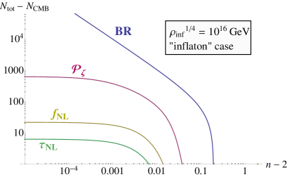
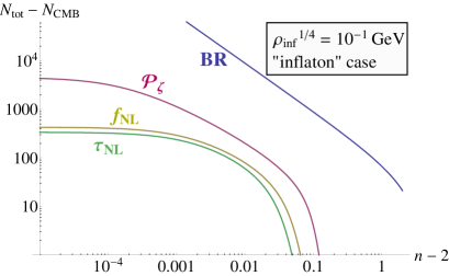
Figure 1: The upper limit of $N_{\rm tot}-N_{\rm CMB}$ for $n\geq 2$ when inflaton generates the observed curvature perturbation. The horizontal axis is $n-2$ and the vertical axis is $N_{\rm tot}-N_{\rm CMB}$. The inflation energy scale is set as $\rho_{\rm inf}^{1/4}=10^{16}$GeV (left panel) or $10^{-1}$GeV (right panel). The blue line denotes the upper limit of $N_{\rm tot}-N_{\rm CMB}$ coming from the back reaction condition, $\rho_{\rm inf}>\rho_{\rm em}$, while the red, yellow and green lines represent the upper limit from the induced $\mathcal{P}_{\zeta}$, $f_{\rm NL}$ and $\tau_{\rm NL}$ from the electromagnetic field respectively. In both panels, one can see that the smaller the $N_{\rm tot}$ or $n-2$ is, the milder the constraints are.

In fig. 1, we plot the upper limit on $N_{\rm tot}-N_{\rm CMB}$ of the “inflaton” case with changing $n$. From these figures, we find that the constraint becomes more stringent as $n$ becomes larger. It is because the generated electric field becomes stronger for larger $n>2$ (see eq. (2.6)) and thus the induced curvature perturbation is amplified. Aside from the back reaction constraint eq. (4.6), the upper limit from m-point correlator contains the factor $\left(\frac{8}{3}c_{n}D_{n}(N_{\rm CMB})\right)^{-m}$ in the argument of logarithm. In case with $n=2$, it reads

$$\left(\frac{8}{3}c_{n}D_{n}(N_{\rm CMB})\ \right)^{-m}\xrightarrow{\scriptstyle n\to 2}\ \left(600\left(\frac{N_{\rm CMB}}{50}\right)\right)^{-m}\qquad(m=2,3,4)$$ (4.10)

and it is even smaller for $n>2$. Because of this factor, the higher $m$ is, the more stringent the constraint is. This behavior can be seen in fig. 1 as the fact that the constraint of $\tau_{\rm NL}$ is the tightest in the left panel. Since low $\rho_{\rm inf}$ corresponds to low $N_{\rm CMB}$ as shown in eq. (4.4), the hierarchy among the constraints derived from $\mathcal{P}_{\zeta},f_{\rm NL}$ and $\tau_{\rm NL}$ is less significant as can be seen in the right panel of fig. 1 where we plot the upper limit of $N_{\rm tot}-N_{\rm CMB}$ for $\rho_{\rm inf}^{1/4}=10^{-1}{\rm GeV}$ case. For $n=2$ case, the upper limit from $\tau_{\rm NL}$ can be obtained from eq. (4.9) as

$$N_{\rm tot}-N_{\rm CMB}\ \lesssim\ 17\times\left(\frac{N_{\rm CMB}}{50}\right)^{-4}\left(\frac{\tau_{\rm NL}^{\rm obs}}{2800}\right),\quad(n=2,\ {\rm``inflaton"\ case})\,.$$ (4.11)

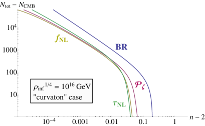
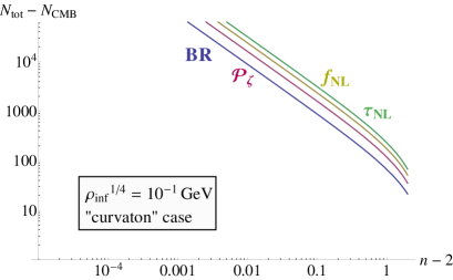
Figure 2: The upper limit of $N_{\rm tot}-N_{{\rm CMB}}$ for $n\geq 2$ when the assumption that inflaton generates the observed curvature perturbation is relaxed. The horizontal axis is $n-2$ and the vertical axis is $N_{\rm tot}-N_{\rm CMB}$. The inflation energy scale and slow-roll parameter are set as $\rho_{\rm inf}^{1/4}=10^{16}$GeV (left panel) or $10^{-1}$GeV (right panel) and $\epsilon=10^{-2}$, respectively. The blue line denotes the upper limit of $N_{\rm tot}-N_{\rm CMB}$ coming from the back reaction condition, $\rho_{\rm inf}>\rho_{\rm em}$, while the red, yellow and green line represent the upper limit from the induced $\mathcal{P}_{\zeta}$, $f_{\rm NL}$ and $\tau_{\rm NL}$ from the electromagnetic field respectively. The back reaction constraint is unchanged from the “inflaton” case since it does not depend on $\epsilon$. But one can see the other three constraints are much milder than those in fig.1.

In fig. 2, we plot the upper limit on $N_{\rm tot}-N_{\rm CMB}$ of the “curvaton” case by setting $\epsilon=10^{-2}$. In this figure, one can see that the constraint is considerably milder than the “inflaton” case. It is interesting to note that the hierarchy among the four constraint is inverted in the low $\rho_{\rm inf}$ plot (right panel). In fact, the upper bound from the back reaction problem is most stringent for $\rho_{\rm inf}^{1/4}\lesssim 10^{15}$GeV. Except for eq. (4.6), the upper limit from m-point correlator contains the factor $\mathcal{P}_{\zeta}^{m-1}/\mathcal{P}_{\rm inf}^{m}$ in the argument of logarithm. Although it reads $\mathcal{P}_{\zeta}^{-1}$ in the “inflaton” case, in the “curvaton” case it yields an extra factor,

$$\left(\frac{\mathcal{P}_{\zeta}}{\mathcal{P}_{\rm inf}}\right)^{m}\simeq\left(18\times\left(\frac{\epsilon}{0.01}\right)\left(\frac{(10^{16}{\rm GeV})^{4}}{\rho_{\rm inf}}\right)\right)^{m}\qquad(m=2,3,4).$$ (4.12)

Therefore the constraints from higher correlator substantially relaxed especially in low $\rho_{\rm inf}$ region. At $\rho_{\rm inf}^{1/4}\simeq 10^{16}$GeV, this factor compensates the factor of eq. (4.10) and three constraints from $\mathcal{P}_{\zeta},f_{\rm NL}$ and $\tau_{\rm NL}$ are almost degenerate (see the left panel). They are coincident with the back reaction constraint at $\rho_{\rm inf}^{1/4}\simeq 10^{15}$GeV. Thus the back reaction bound is the most stringent for $\rho_{\rm inf}^{1/4}\lesssim 10^{15}$GeV.

One can understand why the “curvaton” case with $\epsilon=10^{-2}$ gives much milder bound than the “inflaton” case as follows. From eq. (3.28)-(3.30), one can find $\mathcal{P}_{\zeta}^{\rm em},f^{\rm em}_{\rm NL}$ and $\tau^{\rm em}_{\rm NL}$ are increasing function of $\rho_{\rm inf}$ and decreasing function of $\epsilon$. Thus one way of relaxing the upper limit is to increase $\epsilon$. But $\epsilon$ can not vary freely in the “inflaton” case because $\epsilon$ is determined by $\rho_{\rm inf}$ as

$$\epsilon=5.5\times 10^{-4}\left(\frac{\rho_{\rm inf}}{(10^{16}{\rm GeV})^{4}}\right).$$ (4.13)

Therefore the “curvaton” case does not always put milder constraint than the “inflaton” case but it does only when $\epsilon$ is larger than eq. (4.13).

4.2 Constraint on the inflation energy scale $\rho_{\rm inf}$

If we change the set of input parameters from $\{n,\epsilon,\rho_{\rm inf}\}$ into $\{n,\epsilon,N_{\rm tot}\},$ we can constrain $\rho_{\rm inf}$ instead of $N_{\rm tot}-N_{\rm CMB}$. Although eq. (2.9) gives the upper limit of $\rho_{\rm inf}$ explicitly, we have to numerically calculate the bounds from $\mathcal{P}_{\zeta},f_{\rm NL}$ and $\tau_{\rm NL}$. Provided that $N_{\rm tot}>\frac{3}{2}N_{\rm CMB}$, one can show that the constraints from $\mathcal{P}_{\zeta},f_{\rm NL}$ and $\tau_{\rm NL}$ give upper limits on $\rho_{\rm inf}$. Thus we adopt $N_{\rm tot}=100,300$ and 1000 as the fiducial values. Note the energy scale of inflation is naively restricted by the indirect observation of gravitational wave and the big bang nucleosynthesis as

$$10^{-1}{\rm GeV}\ \lesssim\ \rho_{\rm inf}^{1/4}\ \lesssim\ 10^{16}{\rm GeV}\,,$$ (4.14)

regardless of the kinetic coupling model.

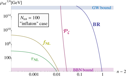
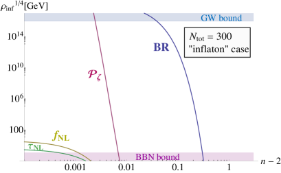
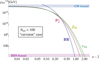
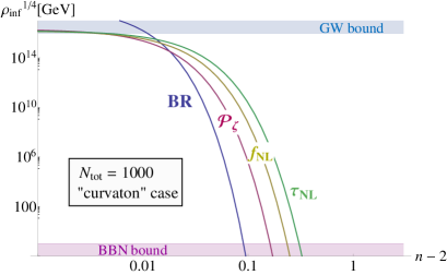
Figure 3: The upper limit of $\rho_{\rm inf}^{1/4}$ for $n\geq 2$. The horizontal axis is $n-2$ and the vertical axis is $\rho_{\rm inf}^{1/4}$ [GeV]. In top two panels it is assumed that inflaton generates all observed curvature perturbation (“inflaton” case) while that assumption is relaxed and instead $\epsilon=10^{-2}$ is adopted in the bottom two panels (“curvaton” case). The total duration of the electromagnetic field generation is set as $N_{\rm tot}=100$ (left panels), 300 (top right panel) or 1000 (bottom right panel). The shaded regions represent the restriction from gravitational wave (blue) and big bang nucleosynthesis (red), respectively.

In fig. 3, we plot the upper limits on $\rho_{\rm inf}^{1/4}$. The basic property of the constraint is unchanged from that on $N_{\rm tot}-N_{\rm CMB}$ because the origin of constraints is same. Again, one can see that the larger $n$ is, the tighter the constraints are. $\tau_{\rm NL}$ gives the most stringent bound in the “inflaton” case while the bound from the back reaction problem is the tightest in low energy region of the “curvaton” case. In addition, now it is clear that the lower $\rho_{\rm inf}$ is, the milder the constraints are. It is remarkable that $N_{\rm tot}\gtrsim 300$ is excluded in the “inflaton” case. It is consistent with the right panel of fig. 1. Even if $N_{\rm tot}<300$, $n$ and $\rho_{\rm inf}$ are severely restricted in the “inflaton” case. On the other hand, the constraints in the “curvaton” case are much more moderate. Especially $\rho_{\rm inf}$ is free from a new restriction if $n$ is sufficiently small. Furthermore, at low energy region, the tightest constraint is given by the back reaction condition whose analytic formula is available. Since in the right hand side of eq. (2.9) the most important factor is $\exp[(2n-4)N_{\rm tot}]$, eq. (2.9) can be approximated by $n-2\lesssim\ln(M_{\rm Pl}^{4}/\rho_{\rm inf})/2N_{\rm tot}$. Then the largest allowed $n$ at $\rho_{\rm inf}^{1/4}=10^{-1}$GeV is

$$n-2\ \lesssim\ \frac{90}{N_{\rm tot}}\,,\qquad({\rm``curvaton"\ case}\,).$$ (4.15)

Since $N_{\rm CMB}$ is as small as $\approx 23$ at such low energy scale, $n$ can be larger than 4 in principle. However, the resultant magnetic field strength at present is depends on $\rho_{\rm inf}$ as $\mathcal{P}_{B}\propto\rho_{\rm inf}^{(n-1)/4}$ and thus a large $n$ does not necessarily lead to a strong magnetic field.

4.3 Constraint on the strength of the magnetic field $B$

In terms of magnetogenesis, it is interesting to put the upper limit on the present strength of the magnetic field, $\mathcal{P}_{B}(\eta_{\rm now},k)$. Combined with eq. (2.7), the upper limits on $\rho_{\rm inf}$ which we obtain in the previous subsection by numerical calculations can be converted into the upper limits on $\mathcal{P}_{B}(\eta_{\rm now},k)$. Those limits are shown in fig. 4.

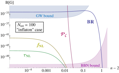
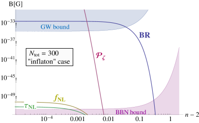
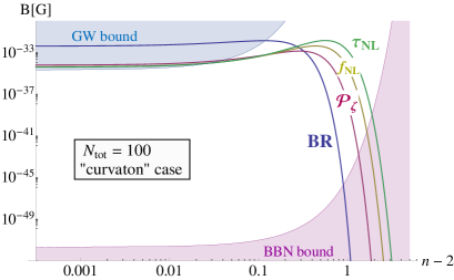
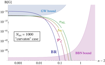
Figure 4: The upper limit of the current strength of the magnetic field for $n\geq 2$. The horizontal axis is $n-2$ and the vertical axis is $\mathcal{P}_{B}^{1/2}(\eta_{\rm now},1{\rm Mpc}^{-1})$ [G]. In top two panels it is assumed that inflaton generates all observed curvature perturbation (“inflaton” case) while that assumption is relaxed and instead $\epsilon=10^{-2}$ is adopted in the bottom two panels (“curvaton” case). The total duration of the electromagnetic field generation is set as $N_{\rm tot}=100$ (left panels), 300 (top right panel) or 1000 (bottom right panel). The shaded region represent the restriction from gravitational wave (blue) and big bang nucleosynthesis (red), respectively.

It is known that the strength of magnetic field generated is kinetic coupling model has been already bounded above due to the back reaction problem and its present value can not exceed $10^{-32}$G for $N_{\rm tot}=70$ and $k=1{\rm Mpc}^{-1}$ [15]. But it turns out that the upper limit is $10^{-47}$G due to the constraint from $\tau_{\rm NL}$ in the “inflaton” case (see the top left panel of fig. 4). If $N_{\rm tot}$ is larger, the constraint becomes even severer. On the other hand, in the “curvaton” case, the strongest value of magnetic field in the allowed region is smaller by only a few orders of magnitude than that without the curvature perturbation constraints.

5 Conclusion

The kinetic coupling model (or $IFF$ model) has drawn attention as both a magnetogenesis model and a generation mechanism of the curvature perturbation and non-gaussianities. Although it is known that the back reaction problem (BR) and the strong coupling problem restrict this model from generating the magnetic field which is strong enough to explain the blazar observation at present, the constraints from the curvature perturbation induced by the electromagnetic fields during inflation are not yet investigated adequately.

In this paper, we compute the curvature power spectrum $\mathcal{P}_{\zeta}$ and non-linear parameters $f_{\rm NL}^{\rm local},\tau_{\rm NL}$ of the curvature perturbation induced by the electromagnetic fields in the kinetic coupling model with $I\propto a^{-n}$ for $n\geq 2$. Quite recently $\mathcal{P}_{\zeta},f_{\rm NL}^{\rm local}$ and $\tau_{\rm NL}$ are precisely determined or constrained by the Planck collaboration. Thus by using the Planck result, we constrain the parameters of the kinetic coupling model and inflation. We find that $\mathcal{P}_{\zeta}^{\rm em},f_{\rm NL}^{\rm em}$ and $\tau_{\rm NL}^{\rm em}$ are given by the functions of four parameters $\{n,N_{\rm tot},\rho_{\rm inf},\epsilon\}$ of the model and inflation (see eq. (3.23), (3.26) and (3.27)). Therefore when three parameters out of four are fixed, the other one can be constrained by the observation. Note in the case where a single slow-rolling inflaton is responsible for all the observed curvature power spectrum, which we call “inflaton” case, the slow-roll parameter $\epsilon$ is determined by inflation energy scale $\rho_{\rm inf}$. On the other hand, if the other mechanism like curvaton or modulated reheating produces observed $\mathcal{P}_{\zeta}$, $\epsilon$ can be a free parameter. For simplicity, this case is called “curvaton” case while we do not specify any model.

In order to illustrate the constraints from the BR, $\mathcal{P}_{\zeta}^{\rm em},f_{\rm NL}^{\rm em}$ and $\tau_{\rm NL}^{\rm em}$, we show three kinds of plot which represent the upper limit of $N_{\rm tot}-N_{\rm CMB},\,\rho_{\rm inf}$ and $\mathcal{P}_{B}^{1/2}(\eta_{\rm now},1{\rm Mpc}^{-1})$ with respect to $n$, respectively. The upper limits of the total e-folding number of magnetogenesis before the CMB scale exits the horizon, $N_{\rm tot}-N_{\rm CMB}$, can be expressed by analytical formula as eq. (4.6)-(4.9). The upper limits of the inflation energy density, $\rho_{\rm inf}$, need numerical calculations to be obtained and can be translated to the upper limits of the present amplitude of the cosmic magnetic field at Mpc scale, $\mathcal{P}_{B}^{1/2}(\eta_{\rm now},1{\rm Mpc}^{-1})$. In general, all four constraints from the BR, $\mathcal{P}_{\zeta}^{\rm em},f_{\rm NL}^{\rm em}$ and $\tau_{\rm NL}^{\rm em}$ become tighter as $n\,(\geq 2)$ is larger. It is simply because the strength of generated electromagnetic fields are amplified as $n\,(\geq 2)$ is larger.

In the “inflaton” case, interestingly, $\tau_{\rm NL}$ gives the strongest limitation on parameters. Even for $\rho_{\rm inf}^{1/4}=10^{-1}{\rm GeV}$ and $n=2$, the constraint from $\tau_{\rm NL}$ puts $N_{\rm tot}\lesssim 300$ and it becomes more stringent for higher $\rho_{\rm inf}$ or $n$. For $N_{\rm tot}=100$ and $n=2$, in turn, $\rho_{\rm inf}^{1/4}\lesssim 10^{4}{\rm GeV}$ is required and $\rho_{\rm inf}$ should be even lower for larger $N_{\rm tot}$ or $n$. As for the magnetic field strength, we find the upper limit from $\tau_{\rm NL}$ is $\mathcal{P}_{B}^{1/2}\lesssim 10^{-47}$G at present Mpc scale for $N_{\rm tot}=100$. It is $10^{-15}$ times lower than the upper limit of the conventional BR condition.

In the “curvaton” case, however, the constraints are more moderate if the free parameter $\epsilon$ is larger than the “inflaton” case. For clarity we fix $\epsilon=10^{-2}$ and show the constraints from $\mathcal{P}_{\zeta}^{\rm em},f_{\rm NL}^{\rm em}$ and $\tau_{\rm NL}^{\rm em}$ are weaker than the BR constraint if $\rho_{\rm inf}$ is sufficiently small. Thus even if the induced curvature perturbation is taken into account, the resultant constraint is not dramatically changed from the conventional BR restriction in the low $\rho_{\rm inf}$ region. In fact, one can see in fig. 4 that the constraint on $\mathcal{P}_{B}$ at present Mpc scale becomes tighter only by $\mathcal{O}(10^{-1})$ than that given solely by the BR.

Aside from the constraints, we find the general relationship between $f_{\rm NL}^{\rm em}$ and $\tau_{\rm NL}^{\rm em}$ in eq. (3.31). According to it, even if $f_{\rm NL}\sim\mathcal{O}(1)$ which is too small to be observed by the Planck satellite, the kinetic coupling model can compatibly produce detectable $\tau_{\rm NL}\gtrsim 560$ [46]. In addition, it is expected that this model generates much higher correlators of the curvature perturbation. Thus it is also interesting to investigate the higher order correlators both in theoretical and observational sides. Furthermore, we use the averaging over the direction of $\hat{\bm{k}}_{i}$ for $f_{\rm NL}$ and $\tau_{\rm NL}$. It should be interesting to consider the direction dependence of $\tau_{\rm NL}$ as well as $f_{\rm NL}$.

References

- [1] B. Ratra, Cosmological ’seed’ magnetic field from inflation, Astrophys. J. 391, L1 (1992).
- [2] B. Himmetoglu, C. R. Contaldi and M. Peloso, Instability of anisotropic cosmological solutions supported by vector fields, Phys. Rev. Lett. 102 (2009) 111301
- [3] D. Lemoine and M. Lemoine, Primordial magnetic fields in string cosmology, Phys. Rev. D 52, 1955 (1995).
- [4] M. Gasperini, M. Giovannini and G. Veneziano, Primordial magnetic fields from string cosmology, Phys. Rev. Lett. 75, 3796 (1995) [hep-th/9504083].
- [5] K. Bamba and J. Yokoyama, Large scale magnetic fields from inflation in dilaton electromagnetism, Phys. Rev. D 69, 043507 (2004)
- [6] K. Bamba and J. Yokoyama, Large-scale magnetic fields from dilaton inflation in noncommutative spacetime, Phys. Rev. D 70, 083508 (2004) [hep-ph/0409237].
- [7] M. A. Ganjali, DBI with primordial magnetic field in the sky, JHEP 0509, 004 (2005) [hep-th/0509032].
- [8] J. Martin and J. ’i. Yokoyama, Generation of Large-Scale Magnetic Fields in Single-Field Inflation, JCAP 0801, 025 (2008) [arXiv:0711.4307 [astro-ph]].
- [9] A. Kandus, K. E. Kunze and C. G. Tsagas, Primordial magnetogenesis, Phys. Rept. 505, 1 (2011)
- [10] M. Giovannini, The Magnetized universe, Int. J. Mod. Phys. D 13, 391 (2004) [astro-ph/0312614].
- [11] A. Neronov and I. Vovk, Evidence for strong extragalactic magnetic fields from Fermi observations of TeV blazars, Science 328, 73 (2010) [arXiv:1006.3504].
- [12] F. Tavecchio, G. Ghisellini, L. Foschini, G. Bonnoli, G. Ghirlanda and P. Coppi, The intergalactic magnetic field constrained by Fermi/LAT observations of the TeV blazar 1ES 0229+200, Mon. Not. Roy. Astron. Soc. 406, L70 (2010) [arXiv:1004.1329].
- [13] A. M. Taylor, I. Vovk and A. Neronov, Extragalactic magnetic fields constraints from simultaneous GeV-TeV observations of blazars, Astron. Astrophys. 529, A144 (2011)
- [14] K. Takahashi, M. Mori, K. Ichiki and S. Inoue, Lower Bounds on Intergalactic Magnetic Fields from Simultaneously Observed GeV-TeV Light Curves of the Blazar Mrk 501, arXiv:1103.3835 [astro-ph.CO].
- [15] V. Demozzi, V. Mukhanov and H. Rubinstein, Magnetic fields from inflation?, JCAP 0908, 025 (2009)
- [16] S. Kanno, J. Soda and M. -a. Watanabe, Cosmological Magnetic Fields from Inflation and Backreaction, JCAP 0912, 009 (2009)
- [17] T. Fujita and S. Mukohyama, Universal upper limit on inflation energy scale from cosmic magnetic field, JCAP 1210, 034 (2012) [arXiv:1205.5031 [astro-ph.CO]].
- [18] M. Giovannini, Electric-magnetic duality and the conditions of inflationary magnetogenesis, JCAP 1004, 003 (2010) [arXiv:0911.0896 [astro-ph.CO]].
- [19] R. J. Z. Ferreira, R. K. Jain and M. S. Sloth, arXiv:1305.7151 [astro-ph.CO].
- [20] T. Suyama and J. ’i. Yokoyama, Metric perturbation from inflationary magnetic field and generic bound on inflation models, Phys. Rev. D 86, 023512 (2012) [arXiv:1204.3976 [astro-ph.CO]].
- [21] M. Giovannini, Fluctuations of inflationary magnetogenesis, Phys. Rev. D 87, 083004 (2013) [arXiv:1302.2243 [hep-th]].
- [22] L. Sorbo, Parity violation in the Cosmic Microwave Background from a pseudoscalar inflaton, JCAP 1106, 003 (2011) [arXiv:1101.1525 [astro-ph.CO]].
- [23] N. Barnaby, J. Moxon, R. Namba, M. Peloso, G. Shiu and P. Zhou, Gravity waves and non-Gaussian features from particle production in a sector gravitationally coupled to the inflaton, Phys. Rev. D 86, 103508 (2012) [arXiv:1206.6117 [astro-ph.CO]].
- [24] M. Giovannini, Transfer matrices for magnetized CMB anisotropies, Phys. Rev. D 73, 101302 (2006) [astro-ph/0604014].
- [25] M. Giovannini, Entropy perturbations and large-scale magnetic fields, Class. Quant. Grav. 23, 4991 (2006) [astro-ph/0604134].
- [26] M. Giovannini, Tight coupling expansion and fully inhomogeneous magnetic fields, Phys. Rev. D 74, 063002 (2006) [astro-ph/0606759].
- [27] M. Giovannini, Large-scale magnetic fields, curvature fluctuations and the thermal history of the Universe, Phys. Rev. D 76, 103508 (2007) [arXiv:0707.0857 [astro-ph]].
- [28] S. Yokoyama and J. Soda, Primordial statistical anisotropy generated at the end of inflation, JCAP 0808, 005 (2008) [arXiv:0805.4265 [astro-ph]].
- [29] M. -a. Watanabe, S. Kanno and J. Soda, The Nature of Primordial Fluctuations from Anisotropic Inflation, Prog. Theor. Phys. 123, 1041 (2010) [arXiv:1003.0056 [astro-ph.CO]].
- [30] R. Emami and H. Firouzjahi, Issues on Generating Primordial Anisotropies at the End of Inflation, JCAP 1201, 022 (2012) [arXiv:1111.1919 [astro-ph.CO]].
- [31] N. Bartolo, S. Matarrese, M. Peloso and A. Ricciardone, The anisotropic power spectrum and bispectrum in the mechanism, Phys. Rev. D 87, 023504 (2013) [arXiv:1210.3257 [astro-ph.CO]].
- [32] R. Emami and H. Firouzjahi, Curvature Perturbations in Anisotropic Inflation with Symmetry Breaking, arXiv:1301.1219 [hep-th].
- [33] M. Karciauskas, K. Dimopoulos and D. H. Lyth, Anisotropic non-Gaussianity from vector field perturbations, Phys. Rev. D 80, 023509 (2009) [Erratum-ibid. D 85, 069905 (2012)] [arXiv:0812.0264 [astro-ph]].
- [34] C. A. Valenzuela-Toledo and Y. Rodriguez, Non-gaussianity from the trispectrum and vector field perturbations, Phys. Lett. B 685, 120 (2010) [arXiv:0910.4208 [astro-ph.CO]].
- [35] E. Dimastrogiovanni, N. Bartolo, S. Matarrese and A. Riotto, Non-Gaussianity and Statistical Anisotropy from Vector Field Populated Inflationary Models, Adv. Astron. 2010, 752670 (2010) [arXiv:1001.4049 [astro-ph.CO]].
- [36] N. Barnaby, R. Namba and M. Peloso, Observable non-gaussianity from gauge field production in slow roll inflation, and a challenging connection with magnetogenesis, Phys. Rev. D 85, 123523 (2012) [arXiv:1202.1469 [astro-ph.CO]].
- [37] M. Shiraishi, E. Komatsu, M. Peloso and N. Barnaby, Signatures of anisotropic sources in the squeezed-limit bispectrum of the cosmic microwave background, arXiv:1302.3056 [astro-ph.CO].
- [38] A. A. Abolhasani, R. Emami, J. T. Firouzjaee and H. Firouzjahi, Formalism in Anisotropic Inflation and Large Anisotropic Bispectrum and Trispectrum, arXiv:1302.6986 [astro-ph.CO].
- [39] R. R. Caldwell, L. Motta and M. Kamionkowski, Correlation of inflation-produced magnetic fields with scalar fluctuations, Phys. Rev. D 84, 123525 (2011) [arXiv:1109.4415 [astro-ph.CO]].
- [40] R. K. Jain and M. S. Sloth, Consistency relation for cosmic magnetic fields, Phys. Rev. D 86, 123528 (2012) [arXiv:1207.4187 [astro-ph.CO]].
- [41] L. Motta and R. R. Caldwell, Non-Gaussian features of primordial magnetic fields in power-law inflation, Phys. Rev. D 85, 103532 (2012) [arXiv:1203.1033 [astro-ph.CO]].
- [42] M. Shiraishi, S. Saga and S. Yokoyama, CMB power spectra induced by primordial cross-bispectra between metric perturbations and vector fields, JCAP 1211, 046 (2012) [arXiv:1209.3384 [astro-ph.CO]].
- [43] D. H. Lyth, K. A. Malik and M. Sasaki, A General proof of the conservation of the curvature perturbation, JCAP 0505, 004 (2005) [astro-ph/0411220].
- [44] P. A. R. Ade et al. [Planck Collaboration], Planck 2013 results. XVI. Cosmological parameters, arXiv:1303.5076 [astro-ph.CO].
- [45] P. A. R. Ade et al. [Planck Collaboration], Planck 2013 Results. XXIV. Constraints on primordial non-Gaussianity, arXiv:1303.5084 [astro-ph.CO].
- [46] N. Kogo and E. Komatsu, Phys. Rev. D 73, 083007 (2006) [astro-ph/0602099].