Abstract

We survey recent results on first-passage processes in unbounded cones and their applications to ordering of particles undergoing Brownian motion in one dimension. We first discuss the survival probability $S(t)$ that a diffusing particle, in arbitrary spatial dimension, remains inside a conical domain up to time $t$. In general, this quantity decays algebraically $S\sim t^{-\beta}$ in the long-time limit. The exponent $\beta$ depends on the opening angle of the cone and the spatial dimension, and it is root of a transcendental equation involving the associated Legendre functions. The exponent becomes a function of a single scaling variable in the limit of large spatial dimension. We then describe two first-passage problems involving the order of $N$ independent Brownian particles in one dimension where survival probabilities decay algebraically as well. To analyze these problems, we identify the trajectories of the $N$ particles with the trajectory of one particle in $N$ dimensions, confined to within a certain boundary, and we use a circular cone with matching solid angle as a replacement for the confining boundary. For $N=3$, the confining boundary is a wedge and the approach is exact. In general, this “cone approximation” gives strict lower bounds as well as useful estimates for the first-passage exponents. Interestingly, the cone approximation becomes asymptotically exact when $N\to\infty$ as it predicts the exact scaling function that governs the spectrum of first-passage exponents.

Chapter 0 First Passage in Conical Geometry and
Ordering of Brownian Particles

1 Introduction

Triggering of earthquakes as stress surpasses a threshold [1], onset of avalanches as mass accumulates beyond stability [2], outbreak of an epidemic once the number infected individuals exceeds a threshold [3], and execution of financial transactions once stock prices reach a prescribed value [4]: All are vivid examples of first-passage processes. Indeed, first-passage processes are ubiquitous and are becoming increasingly relevant for understanding stochastic processes in the physical and the natural sciences [6, 5, 7].

A first-passage process characterizes how a stochastic variable reaches a fixed threshold for the first time. The survival probability $S(t)$ that the threshold is not reached up to time $t$ is a central quantity in the theory of first-passage processes [6, 7]. Basic characteristics follow directly from the survival probability, e.g., $\langle t\rangle=-\int_{0}^{\infty}dt\,t\,(dS/dt)$ measures the average duration of the process; this quantity may be finite or infinite. The first-passage probability that the threshold is ever reached equals $1-S(\infty)$; when $S(\infty)>0$, the threshold may never be reached.

The widely-known gambler ruin problem which involves the location of a simple random walk on a line is a classic first-passage problem. This process ends when the wealth of the gambler reaches either zero or a high threshold [6, 7]. First-passage properties of multiple random walks [8, 9] and particles undergoing Brownian motion [10, 11, 12] in one dimension are the subject of ongoing research and underlie dynamics of spin chains [13, 14, 15], voting processes [16, 17, 18], urn model [19], and unraveling of knots[20]. Many of these first-passage processes are closely related to the ordering of a set of independent Brownian particles on a line [21, 22, 23, 24, 25, 26, 27, 28, 29, 30, 31, 32].

When the number of random walks is no larger than three, first-passage processes involving the order of the particles map onto diffusion in a two-dimensional wedge [21, 27, 28, 7]. For an arbitrary number of particles, a similar mapping remains useful. We recently showed that first-passage processes in high-dimensional cones are connected with a host of problems involving the order of $N$ Brownian particles on a line [33, 34, 35]. In this article, we review these results.

We first discuss the survival probability $S(t)$ that a particle diffusing in an infinite circular $d-$dimensional cone with opening angle $\alpha$ does not cross the cone boundary during the time interval $(0,t)$[36, 37, 38, 39, 40, 41, 42, 43]. The survival probability decays algebraically with time

$$S\sim t^{-\beta}\quad\text{as}\quad t\to\infty.$$ (1)

Since $S(\infty)=0$, the surface of the cone is eventually reached. The exponent $\beta$ turns out to be a root of a transcendental equation involving the associated Legendre functions. We also compute the mean first-passage time which is finite when $\beta>1$.

In principle, the first-passage exponent $\beta$ depends on the opening angle $\alpha$ and the spatial dimension $d$. For $d\gg 1$, the exponent becomes a function of a single scaling variable [44] which is a special combination of $\alpha$ and $d$. The exponent $\beta$ is root of the equation [33]

$$D_{2\beta}(y)=0\quad{\rm with}\quad y=(\cos\alpha)\sqrt{d},$$ (2)

involving the Parabolic cylinder function $D_{\nu}$ [51]. This scaling behavior shows that $\beta$ is of order unity only when the cone is nearly flat (close to a half space). We also discuss a variety of asymptotic properties, e.g., the behavior in the interior and the exterior of very thin cones.

Next, we discuss first-passage processes involving the order $N$ independent Brownian particles in one dimension. We tag the particles according to initial position. Regardless of the initial conditions, the order of the particles eventually gets “scrambled” and since diffusion is an ergodic process, all $N$ permutations of particle order become equally probable. We show that there is a host of interesting first-passage questions that characterize how the initial order unravels.

For example, we rank the particles from right to left according to initial position with rank $n=1$ corresponding to the rightmost particle (the “leader”) and rank $n=N$ to the leftmost particle (the “laggard”). We ask: what is the survival probability $R_{n}(t)$ that the rank of the initial leader at time $t=0$ does not fall below $n$ until time $t$. The quantity $R_{1}$ gives the probability that the leader kept the lead, while $R_{N-1}$ is the probability that the leader is never last [24, 26, 28]. In general, the survival probabilities decay algebraically,

$$R_{n}\sim t^{-\gamma_{n}},$$ (3)

in the long-time limit. Interestingly, there is a family of $N-1$ distinct first-passage exponents with $\gamma_{1}>\gamma_{2}>\cdots>\gamma_{N-1}$.

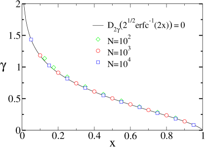
Figure 1: The exponent $\gamma$ versus the scaling variable $x$. Results of Monte Carlo simulations with $N=10^{2}$, $N=10^{3}$, and $N=10^{4}$ particles, are compared with the theoretical prediction (4).

The trajectories of the $N$ one-dimensional Brownian particles can be identified with that of a single compound particle undergoing ordinary Brownian motion in $N$ dimensions. Then $R_{n}$ is the probability that this particle remains within some domain in this higher-dimensional space. When $N\leq 3$, this domain is always a wedge, and the first-passage exponents can be obtained analytically. For arbitrary $N$, we approximate this domain using an unbounded cone that encloses an identical solid angle. This approach gives a useful approximation for the decay exponents $\gamma_{n}$. When the number of particles is very large, we exploit the scaling relationship (2) and find that the exponents $\gamma_{n}$, which depend on the threshold $n$ and the number of particles $N$, become a function of a single scaling variable $n/N$. The exponent $\gamma$ is root of the transcendental equation [34]

$$D_{2\gamma}\left(\sqrt{2}\,{\rm erfc}^{-1}(2x)\right)=0\qquad{\rm with}\qquad x=n/N,$$ (4)

involving the parabolic cylinder function and the inverse complementary error function. As shown in figure 1, numerical simulations reveal that this result is asymptotically exact: The scaling exponent $\gamma_{n}$ is a function of the scaling variable $x=n/N$, and the scaling function is given by (4).

The rest of this paper is organized as follows. In section 2, we provide a pedagogical discussion of first-passage in a two-dimensional wedge. We derive the first-passage exponent directly from the diffusion equation governing the survival probability and show that problems involving particle order map onto a two dimensional wedge when $N=3$. We then generalize this theoretical description to arbitrary spatial dimensions and obtain the first-passage exponent in section 3. Relevant asymptotic relations including in particular the scaling function underlying $\beta$ in the infinite-dimension limit are obtained in section 4. In section 5, we develop the cone approximation, using a three-dimensional corner geometry as an illustrative example. We then discuss rank statistics and use the cone approximation to estimate the first-passage exponents and to derive their asymptotic behavior (section 6). In section 7, we introduce the number of pair inversions as a measure of order. Again, we find that the cone approximation yields useful estimates for the first-passage exponents and that it becomes asymptotically exact when the number of particles diverges. We conclude in section 8.

2 Wedges

Consider a particle undergoing simple diffusion in a wedge (Fig. 2a) with an opening angle $\alpha$. The angle $\alpha$ is measured from the center of the wedge and hence $\alpha\leq\pi$. The first-passage process ends when the particle reaches the boundary of the wedge (Fig. 2b).

The survival probability that the particle avoids the wedge boundary up to time $t$ depends on its initial location $(r,\theta)$ of the particle: $S\equiv S(r,\theta,t)$ where $r$ is the distance to the cone apex and $\theta$ is the polar angle (Fig. 2a). Since the particle undergoes simple Brownian motion, the survival probability obeys the diffusion equation [8]

$$\frac{\partial S(r,\theta,t)}{\partial t}=D\nabla^{2}S(r,\theta,t),$$ (5)

where $D$ is the diffusion coefficient. The boundary condition $S(r,\alpha,t)=0$ reflects that the first-passage process ends when the particle reaches the boundary, and the initial condition is $S(r,\theta,t=0)=1$ for all $\theta<\alpha$.

           

Figure 2: (a) A wedge with opening angle $\alpha$. The radial coordinate $r$ and the polar coordinate $\theta$ specify the initial location of the Brownian particle. (b) Illustration of the first-passage process: the trajectory of a Brownian particle is indicated by a dashed line while the start and end points are indicated by bullets.

The survival probability decays algebraically

$$S(r,\theta,t)\simeq\,\Phi(r,\theta)\,t^{-\beta},$$ (6)

in the long-time limit. The algebraic dependence on time is well-known as for $\alpha=\frac{\pi}{2}$ the problem is effectively one-dimensional and $\beta=\frac{1}{2}$. Here, we show how the decay exponent $\beta$ can be conveniently derived from (5). By substituting the algebraic decay (6) into the diffusion equation (5), we conclude that the amplitude $\Phi$ obeys Laplace’s equation

$$\nabla^{2}\Phi(r,\theta)=0.$$ (7)

The boundary conditions are $\Phi(r,\alpha)=\Phi(0,\theta)=0$. The amplitude must be positive inside the wedge, $\Phi(r,\theta)>0$ for $\theta<\alpha$. The Laplace equation (7) manifests the direct connection between diffusive first-passage processes and electrostatics [9, 45].

Since the quantity $S$ is dimensionless, and since the only dimensionless combination of the quantities $r$, $D$, and $t$ is $Dt/r^{2}$, the amplitude necessarily has the form

$$\Phi(r,\theta)=\left(\frac{r^{2}}{D}\right)^{\beta}\psi(\theta).$$ (8)

The function $\psi\equiv\psi(\theta)$ depends on the polar angle $\theta$ alone. This function is positive inside the wedge, and it vanishes on the boundary, $\psi(\alpha)=0$. We now substitute (8) into (7) and use

$$\nabla^{2}\equiv\frac{\partial^{2}}{\partial r^{2}}+\frac{1}{r}\frac{\partial}{\partial r}+\frac{1}{r^{2}}\frac{\partial^{2}}{\partial\theta^{2}}$$

to find that $\psi(\theta)$ obeys the simple eigenvalue equation

$$\frac{\partial^{2}\psi}{\partial\theta^{2}}+(2\beta)^{2}\psi=0.$$ (9)

Equation (9) involves only the angular component of the Laplacian. By symmetry, we expect that the function $\psi(\theta)$ is even, $\psi(\theta)=\psi(-\theta)$. The solution to Eq. (9) is $\psi(\theta)=\cos(2\beta\theta)$, and the first-passage exponent [46]

$$\beta=\frac{\pi}{4\alpha}$$ (10)

follows immediately from boundary condition $\psi(\alpha)=0$. We see that the asymptotic behavior (6) with the exponent (10) holds for all initial conditions. The initial location affects only the amplitude $\Phi(r,\theta)$. Furthermore, using (6) and (8) we conclude that $S\sim r^{2\beta}$.

The exponent is minimal for a needle, $\beta(\pi)=1/4$ [47], and hence, in two dimensions the particle is bound to encounter a semi-infinite needle [47]. The exponent $\beta(\alpha)$ diverges for infinitely thin wedges, and the duration of the first-passage process is infinitesimal in the limit $\alpha\to 0$. Finally, since $\beta=1$ when $\alpha=\pi/4$, the mean first-passage time is finite if and only if the wedge is smaller than a square corner.

Figure 3: A projection of three dimensional space onto the plane perpendicular to the diagonal line $x_{1}=x_{2}=x_{3}$ divides space into six equal wedges, each with distinct particle order.

First-passage problems involving the order of three particles in one-dimension map onto a wedge. Let $x_{i}(t)$ be the location of the $i$th particle at time $t$. Without loss of generality, we label the particles according to the initial positions, $x_{1}(0)>x_{2}(0)>x_{3}(0)$. Furthermore, we can view the three coordinates $(x_{1},x_{2},x_{3})$ as those of a “composite” particle in three dimensions. Since each particle undergoes independent Brownian motion, the composite particle undergoes Brownian motion in three dimensions. The three planes $x_{1}=x_{2}$, $x_{1}=x_{3}$, and $x_{2}=x_{3}$, divide space into six equal wedges [28, 48] with opening angle $\alpha=\pi/6$ (figure 3), and in each wedge the particle order is distinct.

Consider the rank of the initial rightmost particle. Let $R_{n}$ be the survival probability that this rank does not fall below $n$ up to time $t$. Figure 4a shows the rank of the leader in each of the six wedges. In two of the wedges $n\leq 1$ and in four of them $n\leq 2$. Hence, the survival probabilities $R_{1}$ and $R_{2}$ are equivalent to the probability that a diffusing particle remains inside a wedge with opening angles $\alpha=\pi/3$ and $\alpha=2\pi/3$ respectively. Immediately, we obtain the asymptotic behaviors

$$R_{1}\sim t^{-3/4}\qquad{\rm and}\qquad R_{2}\sim t^{-3/8}.$$ (11)

Using the definition (3), the set of exponents is $\{\gamma_{1},\gamma_{2}\}=\{3/4,3/8\}$. Of course, if there are only two particles, the problem is trivially equivalent to a wedge with opening angle $\alpha=\pi/2$ and the first passage exponent is $\gamma_{1}=1/2$. Based on these two examples, we expect that generally there are $N-1$ exponents $\gamma_{n}(N)$ that obey $\gamma_{1}>\gamma_{2}>\cdots>\gamma_{N-1}$.

                 

Figure 4: (a) The rank $n$ of the initial rightmost particle in each of the six wedges shown in figure 3. (b) The number of inversion $k$ in each of the six wedges.

Figure 3 shows that there is a set of six first-passage exponents

$$\beta_{l}=\frac{3}{2\,l},$$ (12)

where $l=1,2,\ldots,6$ is the number of wedges. Specifically, the set is $\{1/4,3/10,3/8,1/2,3/4,3/2\}$, although for the rank problem, only two of these values are realized.

There are additional measures of particle order, each with a different first-passage process. The rank characterizes only the location of one particle with respect to the rest of the particles. The number of pair inversions, $k$, measures the number of pairs of particles that are inverted with respect to the initial configuration [49, 50]. For example, if the order changes from $321$ initially to $312$ later, then number of inversions increases from $k=0$ to $k=1$ because the pair $12$ is inverted with respect to the initial configuration. The number of inversions is maximal, $k=3$, when the particle order is completely reversed ($321\to 123$) and hence $0\leq k\leq 3$.

What is the survival probability $M_{k}$ that the number of pair inversions remains smaller than $k$ up to time $t$? When $k=0$, the trajectory of the composite particle is confined to a single wedge, $l=1$. Similarly, the condition $k\leq 1$ corresponds to $l=3$, and the condition $k\leq 2$ corresponds to $l=5$. Using equation (12), we find

$$M_{1}\sim t^{-3/2},\qquad M_{2}\sim t^{-1/2},\qquad M_{3}\sim t^{-3/10}.$$ (13)

In section 7, we show that the number of distinct exponents grows quadratically with the number of particles.

3 Circular Cones

An infinite circular cone in arbitrary spatial dimension $d>1$ is specified by the opening angle $\alpha<\pi$, that is, the angle between the cone surface and its axis (see figure 5). The exterior of a cone with opening angle $\alpha$ is a cone with opening angle $\pi-\alpha$. In all dimensions, a cone with opening angle $\alpha=\pi/2$ is a half space.

Figure 5: A cone with opening angle $\alpha$.

The survival probability of a diffusing particle again depends only on two variables: the radial coordinate $r$ and the polar angle $\theta$ (see figure 5). The survival probability obeys the diffusion equation (5) with the Laplacian

$$\nabla^{2}\equiv\frac{\partial^{2}}{\partial r^{2}}+\!\frac{d\!-\!1}{r}\frac{\partial}{\partial r}+\frac{1}{r^{2}(\sin\theta)^{d-2}}\frac{\partial}{\partial\theta}(\sin\theta)^{d-2}\frac{\partial}{\partial\theta}.$$ (14)

In general, the survival probability decays algebraically as in (6) and the amplitude obeys the Laplace equation (7). By following the steps leading to (9) we find that the angular function $\psi$ satisfies the eigenvalue equation

$$\frac{1}{(\sin\theta)^{d-2}}\frac{d}{d\theta}\left[(\sin\theta)^{d-2}\frac{d\psi}{d\theta}\right]+2\beta(2\beta+d-2)\psi=0.$$ (15)

To solve this equation, we introduce the variable $\mu=\cos\theta$, and with this transformation, the function $\psi\equiv\psi(\mu)$ satisfies

$$(1-\mu^{2})\frac{d^{2}\psi}{d\mu^{2}}-(d-1)\,\mu\,\frac{d\psi}{d\mu}+2\beta(2\beta+d-2)\psi=0.$$ (16)

Again, the boundary condition is $\psi(\cos\alpha)=0$.

For $d=3$, the solution to Eq. (16) is given by the Legendre function, $\psi_{3}(\theta)=P_{2\beta}(\cos\theta)$ [51]. The boundary condition implies that the first-passage exponent is the smallest root of the transcendental equation

$$P_{2\beta}(\cos\alpha)=0.$$ (17)

Henceforth, we always choose the smallest root (or equivalently, eigenvalue) because the function $\psi(\theta)$ must remain positive. Further, equation (16) shows that there is a direct connection between the first-passage exponent $\beta$ and the lowest eigenvalue of the angular part of the Laplace operator.

When $d=4$, we can obtain the first-passage exponent explicitly. Using the transformation $\psi_{4}(\theta)=(\sin\theta)^{-1}u(\theta)$, the eigenvalue equation (15) becomes $u_{\theta\theta}+(2\beta+1)^{2}u=0$. There are two independent solutions, $\sin[(2\beta+1)\theta]$ and $\cos[(2\beta+1)\theta]$ but since the function $\psi$ must remain finite, only the former is physical. Therefore $\psi_{4}=\sin\left[(2\beta+1)\theta\right]/\sin\theta$ and the boundary condition $\psi(\alpha)=0$ gives the exponent

$$\beta_{4}(\alpha)=\frac{\pi-\alpha}{2\alpha}\,.$$ (18)

In contrast with equation (10), the exponent now vanishes when $\alpha=\pi$. Hence, in dimensions three and higher, a needle is not reached (Fig. 6). In the limit of very thin cones, the exponent diverges and is inversely proportional to $\alpha$ as in (10). Equations (16)–(17) were recently used for analyzing entropic forces for polymers in the vicinity of a conical tip [42].

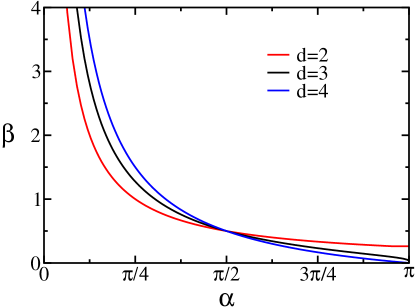
Figure 6: The first-passage exponent $\beta$ versus the opening angle $\alpha$ in dimensions $d=2$, $3$, and $4$.

To solve the eigenvalue equation (16), we make the transformation

$$\psi(\mu)=\left(1-\mu^{2}\right)^{-\delta/2}\Psi(\mu)\qquad{\rm with}\qquad\delta=\frac{d-3}{2}.$$ (19)

The auxiliary function $\Psi(\mu)$ obeys

$$(1-\mu^{2})\frac{d^{2}\Psi}{d\mu^{2}} - 2\,\mu\,\frac{d\Psi}{d\mu}+\left[(2\beta+\delta)(2\beta+\delta+1)-\frac{\delta^{2}}{1-\mu^{2}}\right]\Psi=0.$$ (20)

This equation specifies the associated Legendre functions $P_{2\beta+\delta}^{\delta}(\mu)$ and $Q_{2\beta+\delta}^{\delta}(\mu)$ of degree $2\beta+\delta$ and order $\delta$ [51]. Since $\psi$ must remain finite when $\alpha\to 0$, the first (second) solution is physical when $d$ is odd (even):

$$\psi_{d}(\theta)=\begin{cases}(\sin\theta)^{-\delta}P_{2\beta+\delta}^{\delta}(\cos\theta)&\qquad d~{}~{}{\rm odd},\\ (\sin\theta)^{-\delta}Q_{2\beta+\delta}^{\delta}(\cos\theta)&\qquad d~{}~{}{\rm even}.\end{cases}$$ (21)

Using the fact that the survival probability vanishes on the surface of the cone, we find that $\beta$ is related to the smallest root of the associated Legendre function

$$\begin{split}P_{2\beta+\delta}^{\delta}(\cos\alpha)=0&\qquad d~{}~{}{\rm odd},\\ Q_{2\beta+\delta}^{\delta}(\cos\alpha)=0&\qquad d~{}~{}{\rm even}.\end{split}$$ (22)

In general, the first-passage exponent $\beta\equiv\beta_{d}(\alpha)$ depends on the opening angle $\alpha$ and the dimension $d$. The exponent $\alpha$ decreases monotonically as the opening angle $\alpha$ increases (figure 6).

The solution $\psi_{d}(\mu)$ is polynomial in $\mu$ when the first-passage exponent is half integer. For example, $\psi_{d}(\mu)=\mu$ when $\beta=1/2$ and and $\psi_{d}(\mu)=d\mu^{2}-1$ when $\beta=1$. Hence, the mean-first passage time is finite if only if the opening angle is small enough $\cos\theta>1/\sqrt{d}$.

In general, the mean first-passage time $T(r,\theta)$ for a particle with initial coordinates $(r,\theta)$ obeys the Poisson equation [7, 52]

$$D\nabla^{2}T(r,\theta)=-1,$$ (23)

and satisfies the boundary conditions $T(r,\alpha)=T(0,\theta)=0$. Dimensional analysis implies that $T(r,\theta)=(r^{2}/D)U(\theta)$ with $U$ a dimensionless function of the angle $\theta$. The first-passage time can be obtained explicitly

$$T(r,\theta)=\frac{r^{2}}{2D}\,\frac{\cos^{2}\theta-\cos^{2}\alpha}{d\cos^{2}\alpha-1}.$$ (24)

This equation holds for $\cos\theta>1/\sqrt{d}$ where $\beta>1$. As expected, the duration of the first-passage process is a monotonic function of both distance $r$ and angle $\theta$.

4 Asymptotic properties

Our goal is to apply the first-passage results in unbounded cones to ordering of Brownian particles. We are especially interested in the behavior of a large number of particles, which requires asymptotic properties of (22) when $d\to\infty$. These asymptotics are summarized in this section.

Taking the limit $d\to\infty$ while keeping the angle fixed shows that

$$\lim_{d\to\infty}\beta_{d}(\alpha)=\begin{cases}\infty&\qquad\alpha<\pi/2,\\ 1/2&\qquad\alpha=\pi/2,\\ 0&\qquad\alpha>\pi/2.\\ \end{cases}$$ (25)

Hence, the first-passage process is infinitesimally short when the opening angle is acute, and conversely, it lasts forever when the angle is obtuse. For a right-angle, $\alpha=\pi/2$, the problem is effectively one-dimensional. Further, one can also show [33] that the exponent grows linearly $\beta\sim d$ for acute angles, $\alpha<\pi/2$, while in the complementary case, the exponent decays exponentially, $\beta\sim(\sin\alpha)^{d}$.

The limiting behavior (25) suggests that we should focus on a shrinking region near $\alpha=\pi/2$. Moreover, the fact that $\beta=1$ when $\sqrt{d}\cos\alpha=1$ indicates that the first-passage exponent has the scaling form

$$\beta_{d}(\alpha)\to\beta(y)\qquad{\rm with}\qquad y=(\cos\alpha)\sqrt{d},$$ (26)

when $d\to\infty$. If we take the limits $\mu\to 0$ and $d\to\infty$ in such a way that the scaling variable $z=\mu\sqrt{d}$ is finite, then with this scaling transformation equation (16) becomes

$$\psi_{zz}-z\,\psi_{z}+2\beta\psi=0.$$ (27)

The boundary condition is $\psi(y)=0$. We now make the transformation $\psi(z)=\exp(z^{2}/4)u(z)$ and arrive at the parabolic cylinder equation

$$u_{zz}+\left(2\beta+\frac{1}{2}-\frac{z^{2}}{4}\right)u=0.$$ (28)

The two independent solutions are the parabolic cylinder functions $D_{\nu}(z)$ and $D_{\nu}(-z)$ [51]. Using the asymptotic behavior $D_{\nu}(-z)\sim\exp(z^{2}/4)$ as $z\to\infty$ and the fact that the survival probability must be finite on the cone axis, we eliminate the latter solution and hence,

$$\psi(z)=e^{z^{2}/4}D_{2\beta}(z).$$ (29)

By invoking the boundary condition $\psi(\mu)=0$ we arrive at our main result (2). We choose the largest root of the parabolic cylinder function because $\psi$ is positive. The scaling form (26) implies that $\beta$ is finite in the narrow region of opening angles

$$\alpha-\pi/2\sim d^{-1/2}.$$ (30)

Hence, the first-passage exponent is finite only when the cone is sufficiently close to a half space.

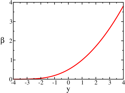
Figure 7: The exponent $\beta$ versus the scaling variable $y=(\cos\alpha)\sqrt{d}$.

Asymptotic analysis of Eq. (29) reveals the limiting behaviors (Fig. 7)

$$\beta(y)\simeq\begin{cases}\sqrt{y^{2}/8\pi}\,\exp\!\left(-y^{2}/2\right)&\qquad y\to-\infty,\\ y^{2}/8&\qquad y\to\infty.\end{cases}$$ (31)

We also mention the asymptotic behaviors in the interior and the exterior of a slender cone (the dimension $d$ is fixed)

$$\beta_{d}(\alpha)\simeq\begin{cases}A_{d}\,\alpha^{-1}&\qquad\alpha\to 0,\\ B_{d}\,(\pi-\alpha)^{d-3}&\qquad\alpha\to\pi.\end{cases}$$ (32)

Inside a very thin cone, the first-passage process is very fast and $\beta$ diverges. The proportionality constant is $A_{d}=\tfrac{1}{2}\zeta(\delta)$ where $\zeta(\delta)$ is the first positive zero of the Bessel[53] function $J_{\delta}$ of order $\delta=\tfrac{d-3}{2}$. For example, $A_{3}\cong 1.202412$, $A_{4}=\frac{\pi}{2}\cong 1.570796$, and $A_{5}\cong 1.915852$. As $\alpha\to\pi$, the exponent $\beta$ vanishes. The coefficient is $B_{d}=\Gamma\big{(}\tfrac{d-2}{2}\big{)}/\big{[}2\,\sqrt{\pi}\,\Gamma\big{(}\tfrac{d-3}{2}\big{)}\big{]}$. The corresponding behavior (32) holds only when $d>3$. For $d=3$, the exponent vanishes logarithmically, $\beta_{3}\simeq 1/[4\ln\frac{2}{\pi-\alpha}]$ (Fig. 6).

5 The cone approximation

The above results for diffusion inside a circular cone can be used to approximate diffusion in more complex geometries for which the eigenvalues of the Laplace operator are not known analytically. We now apply this approach to the exterior of the three-dimensional corner (figure 8). We are interested in the survival probability $S(t)$ of a particle that is diffusing in the exterior of an unbounded corner [54] in dimension three, and we that the powerlaw decay (1) holds, regardless of initial position.

The corner geometry underlies a first-passage problem involving three particles in one dimension. Let’s assume that all particles start in the positive half line, $0<x_{3}(0)<x_{2}(0)<x_{1}(0)$. Then, the probability that the rightmost particle always remains in the positive half line requires that the composite particle remains outside the corner [34]. The complementary problem that the leftmost particle remains in the positive half line is trivial: since all three particles must remain in the positive half space, then $S(t)=[s(t)]^{3}$ with $s(t)\sim t^{-1/2}$ the survival probability in one dimension. Hence, for diffusion inside the corner $\beta=3/2$.

Figure 8: First-passage process outside a three-dimensional corner.

We now replace the corner with an unbounded cone that has identical solid angle. In $d$ dimensions, a cone with opening angle $\alpha$ occupies a fraction $V$ of the total solid angle,

$$V(\alpha)=\frac{\int_{0}^{\alpha}d\theta\,(\sin\theta)^{d-2}}{\int_{0}^{\pi}d\theta\,(\sin\theta)^{d-2}}.$$ (33)

The normalization is such that $V(\pi)=1$, and of course, $V(\pi/2)=1/2$. Equation (33) follows from the Jacobian $d\Omega/d\theta\propto(\sin\theta)^{N-2}$ with $\Omega$ being the solid angle and $\theta$ the polar angle.

By substituting $d=3$ and $V=7/8$ into (33), we find that the equivalent cone has opening angle $\alpha=2.418858$ and from equation (17) we obtain

$$\beta^{\rm cone}=0.216785\qquad{\rm whereas}\qquad\beta=0.228.$$ (34)

The latter value was obtained from numerical simulations (figure 9). Clearly, the cone approximation produces a useful estimate for $\beta$.

The value $\beta^{\rm cone}$ is a lower bound. This assertion follows from the fact that a sphere has the smallest eigenvalue of the Laplace operator amongst the domains with the same volume. In two dimensions, this result was conjectured by Rayleigh [55] and later proved by Faber and Krahn[56]. In higher dimensions, the Rayleigh-Faber-Krahn theorem remains valid [57]. This result implies for example that the ground state of a quantum particle in a box is lowest when the box is spherical; another consequence is that the lifetime of a Brownian particle inside an absorbing box of a fixed volume is highest if the box is spherical. In our situation, we study a composite particle in a general unbounded conical domain in $d$ dimensions. (By definition, any cone $\mathcal{R}$ with an apex at the origin has the property that every ray from the origin to any point inside $\mathcal{R}$ belongs to $\mathcal{R}$.) The eigenvalue problem generalizing Eqs. (9) and (15) arising for circular cones is specified by

$$\nabla^{2}\psi=-2\beta(2\beta+d-2)\psi,\qquad\psi|_{\partial(S^{d-1}\cap\mathcal{R})}=0.$$ (35)

Here $\nabla^{2}$ is the angular component of the Laplacian. The choice of the smallest eigenvalue ensures that the eigenfunction $\psi$ is positive inside $\mathcal{R}$. We need the smallest eigenvalue in the “spherical cap” $S^{d-1}\cap\mathcal{R}$, the intersection of the cone $\mathcal{R}$ with unit sphere $S^{d-1}$, and $\nabla^{2}$ is actually the Laplace-Beltrami operator on the spherical cap. Fortunately, the Rayleigh-Faber-Krahn theorem generalizes to the smallest eigenvalue of the Laplace-Beltrami operator on Riemannian manifolds [57] and it proves that the smallest eigenvalue $2\beta(2\beta+d-2)$, and therefore the smallest $\beta$, amongst all spherical caps with the same volume (i.e., the same solid angle) corresponds to the circular spherical cap. Hence, the cone approximation produces a lower bound.

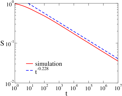
Figure 9: The survival probability in the exterior of a three-dimensional corner. The solid line indicate results of numerical simulations and the dashed line, a best-fit.

Equation (26) shows that for $d\gg 1$, there is universal scaling behavior in terms of the variable $y=(\cos\alpha)\sqrt{d}$. The same scaling variable also underlies the fraction of space $V$ enclosed by the cone. The infinitesimal solid volume element $d\Omega\propto(\sin\theta)^{d-2}d\theta$ in (33) becomes Gaussian, $d\Omega\propto\exp(-y^{2}/2)dy$. Consequently, the volume which depends on the opening angle and the dimension, $V\equiv V(\alpha,d)$, becomes a function of a single variable $y$

$$V(\alpha,d)=\frac{1}{2}\,{\rm erfc}\left(\frac{y}{2}\right).$$ (36)

Here ${\rm erfc}(\xi)=\big{(}2/\sqrt{\pi}\big{)}\int_{\xi}^{\infty}e^{-u^{2}}du$ is the complementary error function. Combining (36) and (4), we find $\beta$ as an implicit function of volume $V$:

$$D_{2\beta}\left(\sqrt{2}\,{\rm erfc}^{-1}(2V)\right)=0.$$ (37)

Remarkably, this expression provides an exact description for the two ordering problems we are interested in.

6 Rank Statistics

We now consider $N$ particles, each undergoing independent Brownian motion in one dimension. The particles are ordered from right to left with the rightmost particle at time $t=0$ regarded as the original leader. As described in the introduction, we are interested in the probability $R_{n}(t)$ that the rank of the original leader does not fall below $n$ up to time $t$ (figure 10). The extremal cases $n=1$ and $n=N-1$ were considered previously [26, 28, 24, 32, 19], yet the long-time kinetics have been established[12] only for $N\leq 3$.

Figure 10: Illustration of the rank problem. Shown is the spacetime diagram of six Brownian particles in one dimension. The particles are ranked according position, from right to left, and in this example, the rank of the leader falls from one to four.

Based on the behavior for $N=3$ where the set $\{\gamma_{1},\gamma_{2}\}=\{3/4,3/8\}$ characterizes the decay $R_{n}\sim t^{-\gamma_{n}}$, we expect $N-1$ distinct exponents,

$$\gamma_{1}>\gamma_{2}>\cdots>\gamma_{N-1}.$$ (38)

Simulation results for $N=4$ confirm this behavior and give (Fig. 11):

$$\gamma_{1}=0.913,\qquad\gamma_{2}=0.556,\qquad\gamma_{3}=0.306.$$ (39)

For $N=4$, the largest exponent has been calculated using electrostatics $\gamma_{1}=0.91342$ [28].

As discussed above, the trajectories of $N$ particles in one dimension can be represented by that of a compound particle in $N$ dimensions. The compound particle is confined to a volume $V_{n}$ of space in which the position of the initial leader is larger than those of at least $N-n$ of the particles. Figure 3 shows that $V_{1}=1/3$ and $V_{2}=2/3$ for $N=3$. Generally

$$V_{n}=\frac{n}{N}.$$ (40)

In $N$ dimensions, the $N(N-1)/2$ hyperplanes $x_{i}=x_{j}$ with $i\neq j$ divide space into $N!$ equal “chambers” each with distinct particle order (figure 2). For example, the region $x_{1}>x_{2}>\cdots>x_{N-1}>x_{N}$ is one such chamber where the initial particle order is preserved, and this chamber occupies a fraction $1/N!$ of the total solid angle. Since there are $(N-1)!$ chambers in which the rank of the original leader equals $1$, then $V_{1}=1/N$. There are $(N-1)!$ additional chambers in which the rank of the leader equals $2$, and hence $V_{2}=2/N$. This argument establishes (40).

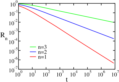
Figure 11: The survival probability $R_{n}$ versus rank $n$ for four particles. The results are obtained from $10^{11}$, $10^{9}$, and $10^{7}$ independent Monte Carlo runs for $n=1$, $n=2$,and $n=3$ respectively.

According to (40), the compound particle is confined to a region of space that is the union of $n(N-1)!$ chambers. To apply the cone approximation, we replace this complex region with an unbounded spherical cone that encloses a fraction $V_{n}$ of space. We set $d=N-1$ so that this approximation is exact when $N=3$. By substituting (40) and $d=N-1$ into (33), we obtain the opening angle $\alpha$. The first-passage exponent is obtained as root of the associated Legendre function specified in (22) with $d=N-1$. For example, when $N=3$, we obtain

$$\gamma^{\rm cone}_{1}=0.888644,\qquad\gamma_{2}=1/2,\qquad\gamma_{3}=0.300754.$$ (41)

These values, which represent formal lower bounds, provide useful estimates for the numerically measured values (39). Table 1 lists the largest and the smallest first-passage exponents for $3\leq N\leq 10$. Although cone approximation slightly deteriorates as the number of particle increases, overall the estimates remain faithful.

The predictions of the cone approximation in the limit $N\to\infty$ follow immediately from equations (40) and (37),

$$D_{2\gamma}\left(\sqrt{2}\,{\rm erfc}^{-1}(2n/N)\right)=0.$$ (42)

The exponent $\gamma$ which depends on two variables, $n$ and $N$, becomes a universal function of the scaling variable $x=n/N$ as stated in equation (4). Remarkably, the scaling function specified by equation (42) is exact! Our numerical simulations which use a remarkably large number of particles (up to $N=10^{4}$) reveal that: (i) the first-passage exponent is a function of the scaling variable $x$, and (ii) the scaling function (42) is exact (figure 1).

The largest and the smallest exponents $\gamma_{1}$ and $\gamma_{N-1}$ for $3\leq N\leq 10$. Simulation results are compared with the outcome of the cone approximation. N $\gamma_{1}^{\rm cone}$ $\gamma_{1}$ $\gamma_{N-1}^{\rm cone}$ $\gamma_{N-1}$ $3$ $3/4$ $3/4$ $3/8$ $3/8$ $4$ $0.888644$ $0.91$ $0.300754$ $0.306$ $5$ $0.986694$ $1.02$ $0.253371$ $0.265$ $6$ $1.062297$ $1.11$ $0.220490$ $0.234$ $7$ $1.123652$ $1.19$ $0.196216$ $0.212$ $8$ $1.175189$ $1.27$ $0.177469$ $0.190$ $9$ $1.219569$ $1.33$ $0.162496$ $0.178$ $10$ $1.258510$ $1.37$ $0.150221$ $0.165$

This finding may indicate that in very high dimensions, the complex boundary confining the composite particle approaches a limiting shape, and that this limiting shape is conical. Another possible scenario is that the complex boundary, which is formed by the intersection of multiple hyperplanes, does not necessarily approach a limiting conical shape, yet the deviations do not affect lowest eigenvalue of the Laplace operator.

The scaling function (42) manifests that there is a continuous spectrum of first-passage exponents $0<\gamma<\infty$ when $N\to\infty$. The smallest exponent vanishes as $N^{-1}$, while the largest diverges logarithmically. More precisely,

$$\gamma_{n}\simeq\begin{cases}\frac{1}{4}\ln N&\qquad n=1,\\ \frac{1}{N}\ln N&\qquad n={N-1}.\end{cases}$$ (43)

These limiting behaviors follow from asymptotic analysis of (42) with $n=1$ and $n=N-1$, and in both cases, we recover results obtained using heuristic scaling arguments [26, 28]. We also note that median exponent, which characterizes the probability that the leader always ranks above the median particle, approaches the simple limit $\gamma_{N/2}\to 1/2$.

Knowledge of the scaling form (42), merely the fact that $\gamma$ is function of the variable $x=n/N$ is quite powerful. This realization enables measurement of first-passage exponents for up to $N=10^{4}$ particles, corresponding to diffusion in a staggering spatial dimension $d=10^{4}$. Whereas accurate measurement of the (vanishing) smallest or the (diverging) largest exponent become prohibitive [24] already at $N\approx 10$, we are able to compute $\gamma$ by measuring the probability that the rank of the original leader remains in the first percentile rather than strictly remaining first. The numerical simulation also show that not only does the first-passage exponent becomes a function of the scaling variable $x=n/N$, but so does the entire survival probability: $R_{n}(N,t)\to\Phi(x,t)$ with $x=n/N$ in the limit $N\to\infty$.

7 Inversion Statistics

Rank compares the location of a single particle, the initial leader, with those of the rest of the particles. Generally, there are $N(N-1)/2$ distinct pairs, and the number of pair inversion $k$ treats all particles equally. If initially the particle locations are such that $x_{N}(0)<x_{N-1}(0)<\cdots<x_{1}(0)$, then the number of pair inversions is

$$k(t)=\sum_{i\neq j}\Theta\big{(}x_{i}(t)-x_{j}(t)\big{)},$$ (44)

with $\Theta(x)$ the step function: $\Theta(x)=1$ when $x>0$ and $\Theta(x)=0$ otherwise. In figure 12 the initial order is $4321$ and later, when the order becomes $2341$, the number of inversions equals $k=3$ as the pairs $23$, $24$, and $34$ are inverted with respect to the initial configuration. The number of inversions (also known as the Mahonian number) is a basic measure of a permutation, and it is routinely used in sorting and ranking algorithms [6, 58, 59, 49]. The number of inversions lies between $0$ and $N(N-1)/2$.

There are $N!$ different permutations of particle order and since the diffusion process is ergodic, all of these permutations become equally probable. It is easy to show that if initially the particles are regularly spaced, the “equilibration” time is quadratic in $N$ [35]. Consequently, the equilibrium distribution of the inversion number is given by the well-known Mahonian probability distribution $P_{k}(N)$ that a random permutation of $N$ integers has $k$ inversions. The generating function reads [50]

$$\sum_{k}P_{k}(N)s^{k}=\frac{1}{N!}\prod_{n=1}^{N}(1+s+s^{2}+\cdots+s^{n-1}).$$ (45)

From this generating function, we can obtain the distribution function. For example, for two particles, $P_{0}(2)=P_{1}(2)=1/2$, and for three particles, $P_{0}(3)=P_{2}(3)=1/6$ while $P_{1}(3)=P_{2}(3)=1/3$ (figure 4b). We are particularly interested in the cumulative distribution $V_{k}(N)$ that the number of inversions is smaller than $k$

$$V_{k}(N)=\sum_{j<k}P_{j}(N).$$ (46)

Figure 12: Illustration of the inversion problem. Shown is the spacetime diagram of four particles in one dimension. The number of inversions grows from $k=0$ to $k=3$.

From the generating function (45), we can obtain the average number of inversions $\langle k\rangle$ and the standard deviation $\sigma$:

$$\langle k\rangle=\frac{N(N-1)}{4}\qquad{\rm and}\qquad\sigma^{2}=\frac{N(N-1)(2N+5)}{72}\,.$$ (47)

Notably, the standard deviation is large, $\sigma\sim N^{3/2}$. When the number of particles is large, the distribution $P_{k}$ becomes normal and is characterized by the mean and the standard deviation [6, 60]. Consequently, the cumulative probability $V_{k}(N)$ that the inversion number is $\leq k$ approaches the complementary error function in the $N\to\infty$ limit:

$$V_{k}(N)\to{\rm erfc}\left(-\frac{w}{\sqrt{2}}\right)\qquad{\rm with}\qquad w=\frac{k-\langle k\rangle}{\sigma}\,.$$ (48)

Let $M_{k}(t)$ be the survival probability that the number of inversions remains smaller than $k$ up to time $t$. We anticipate

$$M_{k}\sim t^{-\nu_{k}}\qquad\text{with}\qquad\nu_{1}>\cdots>\nu_{N(N-1)/2}.$$ (49)

Equation (13) shows that $\{\nu_{1},\nu_{2},\nu_{3}\}=\{3/2,1/2,3/10\}$ when $N=3$. Numerical simulations confirm that the number of distinct exponents equals $N(N-1)/2$. In contrast with the rank statistics above, the number of distinct exponents is quadratic in $N$.

First-passage exponents for four particles. Results of Monte Carlo simulations, $\nu_{k}$ versus the outcome of the cone approximation, $\nu_{k}^{\rm cone}$. $k$ $1$ $2$ $3$ $4$ $5$ $6$ $\nu_{k}^{\rm cone}$ $2.67100$ $1.17208$ $0.64975$ $0.39047$ $0.24517$ $0.14988$ $\nu_{k}$ $3$ $1.39$ $0.839$ $0.455$ $0.275$ $0.160$

The quantity $M_{1}$ equals the probability that the particle order remains intact, and the respective exponent $\nu_{1}$ is known analytically [21, 22, 23, 61, 25, 29]

$$\nu_{1}=\frac{N(N-1)}{4}.$$ (50)

When $k=1$, the trajectory of the compound Brownian particle is confined to one chamber, $x_{1}>x_{2}>\cdots>x_{N}$.

We again use the cone approximation to estimate the first-passage exponents. The fraction (46) calculated from the generating function (45) is substituted into (33) to give the opening angle $\alpha$. Using this angle and $d=N-1$, we deduce the exponent from equation (22). Results of the cone approximation for the case $N=4$ are listed in table 2. Again, we obtain useful estimates for the first-passage exponents.

To obtain the limiting behavior when the number of particles diverges, $N\to\infty$, we substitute (48) into the scaling relation (4). The scaling exponent $\nu$ becomes a function of the scaling variable $w$ defined in (48) and is root of the parabolic cylinder equation,

$$D_{2\nu}(-w)=0.$$ (51)

Hence, if we focus on the probability that the number of inversions does not exceed a fixed number $w$ of standard deviations from the mean, the first-passage process becomes independent of the number of particles. This realization is especially useful in the case of inversion statistics: the family of exponents is quadratic in $N$, and furthermore, the scaling variable $w$ guides us to measure $\nu_{k}$ in a scaling window of size $N^{3/2}$ around the average, $\langle k\rangle\simeq N^{2}/4$. Indeed, by using a finite number of measurements, we can verify that $\nu\equiv\nu_{k}(N)$ becomes a function of the scaling variable $w$. Again, the cone approximation predicts the exact scaling function governing $\nu$ (figure 13).

     

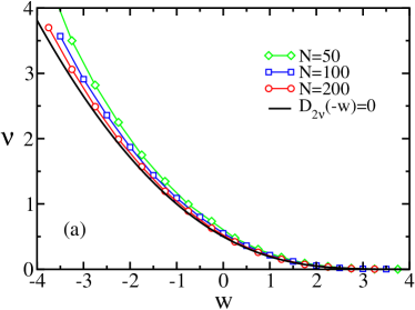
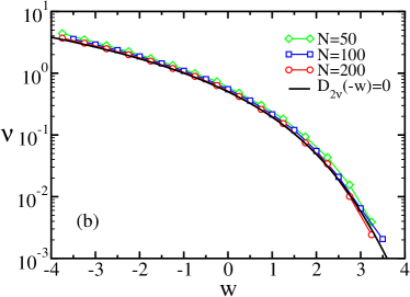
Figure 13: The exponent $\nu$ versus the scaling variable $w$. Predictions of the cone approximation are compared with results of Monte Carlo simulations with $N=50$, $N=100$, and $N=200$ particles.

8 Conclusions

We studied first-passage properties of a Brownian particle in unbounded circular cones. The first-passage exponent characterizing the decay of the survival probability is root of a transcendental equation involving the associated Legendre equation. Explicit expressions for this exponent are feasible only in two and four dimensions. Another simplification occurs when $d\gg 1$ where the exponent, which generally depends on the cone opening angle $\alpha$ and $d$, becomes a function of a single variable $\sqrt{d}\,\cos\alpha$. This universal function is obtained analytically as a root of the parabolic cylinder function.

We analyzed two first-passage problems involving the order of an ensemble of independent Brownian particles in one dimension. The trajectories of the $N$ Brownian particles define a compound trajectory of a single Brownian particle in $N$ dimensions, more precisely in an infinite cone with numerous plane boundaries. As an approximation, we replaced this cone with complex boundary by a circular cone having an identical solid angle. We showed that the cone approximation yields a lower bound and surprisingly good approximations for the first-passage exponents.

There are families of first-passage exponents that govern kinetics of ordering of Brownian particles or equivalently, kinetics of first-passage in high dimensions. We discussed only two out of many possible measures for particle order: the rank of the original leader and the number of pair inversions. In one case, the number of first-passage exponents is linear in the number of particles; in the other case, it is quadratic. The discrete spectrum of exponents becomes continuous when the number of particles diverges. Surprisingly, the cone approximation predicts this spectrum exactly.

An important challenge is to establish when does the confining geometry becomes equivalent to a cone in a high-dimensional space and the conditions for the cone approximation to be asymptotically exact. We presented two cases for which the scaling function is predicted exactly, but there are counterexamples where the cone approximation correctly predicts the scaling form but fails to predict the actual scaling function [34].

The exponents exhibit scaling when the number of particles diverges. This realization is relevant for numerical simulations [62, 63] where it is difficult to measure exponents that are either much smaller than or much larger than unity. The scaling variable specifies the region where the first-passage exponents are of order one. For example, for the rank problem the scaling behavior implies that the rank should be measured in percentiles.

First-passage processes are inherently nonequilibrium. By definition the particle trajectory is restricted to certain regions in space whereas other regions are strictly excluded. For example, in the corner geometry (8) an unrestricted Brownian particle visits all eight “quadrants” with equal probabilities $p=1/8$. Yet, for first-passage processes inside a three-dimensional corner, we have $p=1$ inside the corner and $p=0$ otherwise. By exploiting the cone geometry, we have shown that the equilibrium probabilities (40) and (48) translate into knowledge of nonequilibrium properties, and in particular, first-passage exponents. Interestingly, geometrical properties allow us to deduce exact nonequilibrium properties of a particle system from its equilibrium properties. It will be interesting to extend these results to other geometries [64, 65] and to establish connections with other problems involving ordering of Brownian particles.

We acknowledge DOE grant DE-AC52-06NA25396 for support.

References

- 1. M. Ohnakam, The Physics of Rock Failure and Earthquakes (Cambridge University Press, Cambridge 2013).
- 2. P. Bak, How nature works: the science of self-organized criticality (Copernicus, New York, 1999).
- 3. J. D. Murray, Mathematical Biology (Springer, Berlin 1989)
- 4. J.-P. Bouchaud and M. Potters, Theory of Financial Risk and Derivative Pricing (Cambridge University Press, Cambridge 2003).
- 5. N. G. van Kampen, Stochastic Processes in Physics and Chemistry (North Holland, Amsterdam, 2003).
- 6. W. Feller, An Introduction to Probability Theory and Its Applications (Wiley, New York, 1968).
- 7. S. Redner, A Guide to First-Passage Processes (Cambridge University Press, New York, 2001).
- 8. G. H. Weiss, Aspects and Applications of the Random Walk (North-Holland, Amsterdam, 1994).
- 9. H. C. Berg, Random Walks in Biology (Princeton University Press, Princeton, 1983).
- 10. B. Duplantier, in: Einstein, 1905-2005, eds. Th. Damour, O. Darrigol, B. Duplantier and V. Rivasseau (Birkhäuser Verlag, Basel, 2006); arXiv:0705.1951.
- 11. P. Mörders and Y. Peres, Brownian Motion (Cambridge University Press, Cambridge, 2010).
- 12. P. L. Krapivsky, S. Redner, and E. Ben-Naim, A Kinetic View of Statistical Physics (Cambridge University Press, Cambridge, 2010).
- 13. B. Derrida, V. Hakim, and V. Pasquier, Phys. Rev. Lett. 75, 751 (1995).
- 14. S. N. Majumdar, C. Sire, A. J. Bray, and S. J. Cornell, Phys. Rev. Lett. 77, 2867 (1996); B. Derrida, V. Hakim, and R. Zeitak, Phys. Rev. Lett. 77, 2871 (1996).
- 15. A. J. Bray, S. N. Majumdar, and G. Schehr, arXiv:1304.1195.
- 16. P. L. Krapivsky, E. Ben-Naim, and S. Redner, Phys. Rev. E 50, 2474 (1994).
- 17. M. Howard and C. Godreche, J. Phys. A 31, L209 (1998).
- 18. H. Niederhausen, Eur. J. Combinatorics 4, 161 (1983).
- 19. T. Antal, E. Ben-Naim, and P. L. Krapivsky, J. Stat. Mech. P07009 (2010).
- 20. E. Ben-Naim, Z. A. Daya, P. Vorobieff, and R. E. Ecke, Phys. Rev. Lett. 86, 1414 (2001).
- 21. M. E. Fisher, J. Stat. Phys. 34, 667 (1984).
- 22. D. A. Huse and M. E. Fisher, Phys. Rev. B 29, 239 (1984).
- 23. M. E. Fisher and M. P. Gelfand, J. Stat. Phys. 53, 175 (1988).
- 24. M. Bramson and D. Griffeath, in: Random Walks, Brownian Motion, and Interacting Particle Systems: A Festshrift in Honor of Frank Spitzer, eds. R. Durrett and H. Kesten (Birkhäuser, Boston, 1991).
- 25. D. J. Grabiner, Ann. Inst. Poincare: Prob. Stat. 35, 177 (1999).
- 26. P. L. Krapivsky and S. Redner, J. Phys. A 29, 5347 (1996); S. Redner and P. L. Krapivsky, Amer. J. Phys. 67, 1277 (1999).
- 27. D. ben-Avraham, J. Chem. Phys. 88, 15 (1988).
- 28. D. ben-Avraham, B. M. Johnson, C. A. Monaco, P. L. Krapivsky, and S. Redner, J. Phys. A 36, 1789 (2003).
- 29. J. Cardy and M. Katori, J. Phys. A 36, 609 (2003).
- 30. D. L. Burkholder, Adv. Math. 26, 182 (1977).
- 31. S. B. Yuste, L. Acedo, and K. Lindenberg, Phys. Rev. E 64, 052102 (2001).
- 32. D. ben-Avraham, S. N. Majumdar, and S. Redner, J. Stat. Mech. L04002 (2007).
- 33. E. Ben-Naim and P. L. Krapivsky, J. Phys. A 43, 495007 (2010).
- 34. E. Ben-Naim and P. L. Krapivsky, J. Phys. A 43, 495008 (2010).
- 35. E. Ben-Naim, Phys. Rev. E 82, 061103 (2010).
- 36. R. D. DeBlassie, Probab. Theory Relat. Fields 74, 1 (1987); Probab. Theory Relat. Fields 79, 95 (1988).
- 37. B. Davis and B. Zhang, Proc. AMS 121, 925 (1994).
- 38. R. Bañuelos and R. G. Smiths, Probab. Theory Relat. Fields 108, 299 (1997).
- 39. R. Bañuelos, R. D. DeBlassie, and R. G. Smiths, Ann. Probab. 29, 882 (2001).
- 40. N. Th. Varopoulos, Math. Proc. Camb. Phi. Soc. 125, 335 (1999); Math. Proc. Camb. Phi. Soc. 129, 301 (1999).
- 41. J. H. Jeon, A. V. Chechkin, and R. Metzler, EPL 94, 20008 (2011).
- 42. M. F. Maghrebi, Y. Kantor, and M. Kardar, EPL 96, 66002 (2011); Phys. Rev. E 86, 061801 (2012).
- 43. E. K. Lenzi, L. R. Evangelista, M. K. Lenzi, and L. R. da Silva, Phys. Rev. E 80, 021131 (2011).
- 44. G. I. Barenblatt, Scaling, Self-Similarity, and Intermediate Asymptotics (Cambridge University Press, Cambridge, 1996).
- 45. J. D. Jackson, Classical Electrodynamics (Wiley, New York, 1998).
- 46. F. Spitzer, Trans. AMS 87, 187 (1958).
- 47. D. Considine and S. Redner, J. Phys. A 22, 1621 (1988).
- 48. D.L. L. Dy and J. P. Esguerra, Phys. Rev. E 78, 062101 (2008).
- 49. M. Bóna, Combinatorics of Permutations (Chapman and Hall, Boca Raton, 2004).
- 50. D. E. Knuth, The Art of Computer Programming, vol. 3: Sorting and Searching (Addison-Wesley, New York, 1998).
- 51. NIST Handbook of Mathematical Functions, ed. F. W. J. Olver, D. M. Lozier, et al. (Cambridge University Press, Cambridge, 2010).
- 52. T. G. Mattos, C. Mejia-Monasterio, R. Metzler, and G. Oshanin, Phys. Rev. E 86, 031143 (2012).
- 53. J. D. Watson, A Treatise on the Theory of Bessel Functions (Cambridge University Press, Cambridge, 1995).
- 54. L. C. Davis and J. Reitz, J. Math. Phys. 16, 1219 (1975).
- 55. J. W. S. Rayleigh, The Theory of Sound (Macmillan, New York, 1877; reprinted Dover, New York, 1945).
- 56. R. Courant and D. Hilbert, Methods of Mathematical Physics, vol. I (Wiley, New York, 1953).
- 57. I. Chavel, Eigenvalues in Riemannian geometry (Academic Press, Orlando, 1984).
- 58. P. A. McMahon, Amer. J. Math. 35, 281 (1913).
- 59. G. E. Andrews, The Theory of Partitions (Addison-Wesley, Reading, 1976).
- 60. R. E. Canfield, S. Janson, and D. Zeilberger, Adv. Appl. Math. 49, 77 (2010).
- 61. I. M. Gessel and D. Zeilberger, Proc. Amer. Math. Soc. 115, 27 (1992).
- 62. P. Grassberger, Computer Phys. Comm. 147, 64 (2002).
- 63. T. Oppelstrup, V. V. Bulatov, A. Donev, M. H. Kalos, G. H. Gilmer, and B. Sadigh, Phys. Rev. E 80, 066701 (2009).
- 64. M. Lifshits and Z. Shi, Bernoulli 8, 745 (2002).
- 65. P. L. Krapivsky and S. Redner, J. Stat. Mech. P11028 (2010).