Cache-Enabled Opportunistic Cooperative MIMO for Video Streaming in Wireless Systems

Abstract

We propose a cache-enabled opportunistic cooperative MIMO (CoMP) framework for wireless video streaming. By caching a portion of the video files at the relays (RS) using a novel MDS-coded random cache scheme, the base station (BS) and RSs opportunistically employ CoMP to achieve spatial multiplexing gain without expensive payload backhaul. We study a two timescale joint optimization of power and cache control to support real-time video streaming. The cache control is to create more CoMP opportunities and is adaptive to the long-term popularity of the video files. The power control is to guarantee the QoS requirements and is adaptive to the channel state information (CSI), the cache state at the RS and the queue state information (QSI) at the users. The joint problem is decomposed into an inner power control problem and an outer cache control problem. We first derive a closed-form power control policy from an approximated Bellman equation. Based on this, we transform the outer problem into a convex stochastic optimization problem and propose a stochastic subgradient algorithm to solve it. Finally, the proposed solution is shown to be asymptotically optimal for high SNR and small timeslot duration. Its superior performance over various baselines is verified by simulations.

I Introduction

Nowadays, more and more high data rate applications, such as video streaming, are supported by wireless networks. It is envisioned that future 5G wireless systems should offer 1000X increase in capacity. One key technology to achieve this challenging goal is by means of cooperative MIMO (CoMP) [1, 2] because it can transform the cross-link interference into spatial multiplexing gain. However, CoMP technique requires high capacity backhaul for payload exchange between BSs, which is a cost bottleneck for large scale deployment of CoMP in dense small cell networks. On the other hand, cooperative relay has been proposed as an alternative technique to improve the performance of wireless networks without expensive backhaul. However, it can only contribute to coverage and SNR gain and the overall capacity gain is marginal [3, 4].

In this paper, we propose a novel solution framework, namely the cache-enabled opportunistic CoMP, to fully unleash the benefits of CoMP without expensive payload backhaul. By introducing cache at the relay (RS), we can opportunistically transform a relay channel into a CoMP broadcast channel and achieve not only SNR gain but also spatial multiplexing gain. Due to the absence of payload backhaul, such a solution is very attractive for dense small cell networks. In traditional wireless networks, the information bits are treated as random bits and hence, the capacity is limited by the underlying network topology. However, in future wireless networks, the source should be viewed as content rather than random bits. For example, it is envisioned that a significant portion of the 1000X capacity demand in 5G systems comes from video streaming applications. As such, a large portion of video traffic corresponds to a few popular video files which are requested by many users. There are huge correlations between the information accessed by users and such information is cachable at the RS. If a user accesses a content which exists in the RS cache, the BS and the RS can engage in CoMP and therefore, enjoy spatial multiplexing gain in addition to SNR gain. Hence, with proper caching strategy, a large portion of backhaul usage can be replaced by the cache. Since the cost of hard disks is much lower than the cost of optical fiber backhaul, the proposed solution is very cost effective.

Yet, the opportunity of CoMP in the information flows depends heavily on the dynamic caching strategy. Caching has been widely used in fixed line P2P systems [5, 6] and content distribution networks (CDNs) [7, 8]. The benefits of caching in these cases mainly come from reducing the number of hops from the content source to the consumers. However, we have a fundamentally different caching cost and reward dynamics in the wireless scenario. In addition to the common advantage of bringing the content close to the consumers, there is a unique advantage of cache-induced topology change in the physical layer (dynamic CoMP opportunity) of the wireless systems. As such, one cannot directly adopt conventional caching algorithms in the fixed line networks. In [9], a FemtoCaching scheme is proposed by using small BSs called helpers with high storage capacity cache popular video files. However, the FemtoCaching scheme does not consider cache-enabled opportunistic CoMP among the BS and local helpers. Hence, the cache control in [9] is independent of the physical layer and is fundamentally different from our case where the cache control and physical layer are coupled together. In our recent paper [10], we studied a mixed-timescale optimization of MIMO precoding and cache control for MIMO interference networks employing the cache-enabled opportunistic CoMP. However, the cache control and MIMO precoding algorithms in [10] can only be used to guarantee the physical layer QoS (fixed data rate requirement for each user) and the MIMO precoder is not adaptive to the QSI at the mobile users.

In this paper, we study two timescale joint optimization of power and cache control to support real-time video-on-demand (VoD) applications. The role of cache control is to create (induce) more CoMP opportunities and is adaptive to long-term popularity of the video files (long-term control). The role of dynamic power control is to exploit the CoMP opportunities (induced by the cache) to strike a balance between capacity gain and the urgency between information flows. As such, it is adaptive to the instantaneous CSI, the cache state at the RS and the QSI at the mobile users. There are several technical challenges to be addressed.

• Cache Size Requirement: The performance gain of the proposed scheme depends heavily on the CoMP opportunity, which in turn depends on the cache size and cache algorithm. The RS usually does not have enough cache to store all the video files. As will be shown in Example 1, when brute force caching is used, even if a significant portion of the video files are cached at RS, the CoMP opportunity can still be very small and this is highly undesirable.

• Unknown Video File Popularity: In many cases, the RS does not have the knowledge of the popularity of the video files. Hence, the cache control must have the ability to automatically learn the popularity of video files.

• Challenge of QoS Requirement: It is important to dynamically control the transmit powers at the BS and the RS based on the CSI, cache state (reveals good opportunities of transmission) and the QSI (reveals urgency of the data flow) at the mobile in order to maintain low interruption probability during video playback. Yet, the optimization belongs to the infinite horizon Markov Decision Process (MDP) [11, 12], which is well-known to be very challenging.

• Complex Coupling between Cache and Power Control: The cache control will affect the physical layer dynamics seen by power control due to different CoMP opportunities. Furthermore, the optimization objective of the cache control (long-term) depends on the optimal power solution as well as the average cost of the MDP. However, there are no closed-form characterizations for them.

To address the above challenges, we first propose a novel cache data structure called MDS-coded random cache which can significantly improve the probability of CoMP. We then exploit the timescale separations of the control variables to decompose the problem into an inner power control problem and an outer cache control problem. To solve the inner power control problem, we exploit a specific problem structure and derive an approximate Bellman equation. Based on this, we derive a closed-form approximation for the value function, the power control policy as well as the average cost. To solve the outer cache control problem, we exploit these closed form approximations for the inner problem and transform the outer problem into a convex stochastic optimization problem. Then we propose a stochastic subgradient algorithm to solve it. We show that the proposed solution is asymptotically optimal for high SNR and small timeslot duration. Finally, we illustrate with simulations that the proposed solution achieves significant gain over various baselines.

Notations: The superscript $\left(\cdot\right)^{\dagger}$ denotes Hermitian. The notation $1\left(\cdot\right)$ denote the indication function such that $1\left(E\right)=1$ if the event $E$ is true and $1\left(E\right)=0$ otherwise. The notation $\textrm{span}\left(\mathbf{A}\right)$ represents the subspace spanned by the columns of a matrix $\mathbf{A}$.

II System Model

In this section, we introduce the architecture of the video streaming system, the physical layer (opportunistic CoMP), the MDS-coded random cache scheme that supports opportunistic CoMP, and the queue model.

II-A Architecture of Video Streaming System

The architecture of the video streaming system is illustrated in Fig. 1. There are $L$ video files on the VoD server. The size of the $l$-th video file is $F_{l}$ bits. For simplicity, we assume that the $L$ video files have the same streaming rate denoted by $\mu_{0}$ (bits/s). There are $2M$ users streaming video files from the VoD server via a radio access network (RAN) consisting of an $M$-antenna BS and an $M$-antenna RS. The index of the video file requested by the $k$-th user is denoted by $\pi_{k}$. Define $\pi=\left\{\pi_{1},...,\pi_{2M}\right\}$ as the user request profile (URP). We have the following assumption on URP.

Assumption 1 (URP Assumption).

The URP $\pi\left(t\right)$ is a slow ergodic random process (i.e., $\pi\left(t\right)$ remains constant for a large number of time slots) according to a general distribution.

Video packets are delivered to the BS from the VoD gateway via the high speed backhaul as illustrated in Fig. 1. On the other hand, the RS has no fixed line backhaul connection with the BS and it is equipped with a cache. In this paper, the time is partitioned into time slots indexed by $t$ with slot duration $\tau$.

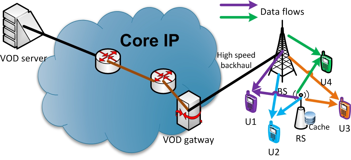
Figure 1: The architecture of the video streaming system.

II-B Cache-enabled Opportunistic CoMP

The RAN is the performance bottleneck of the system. Without cache at the RS, the RAN forms a MIMO relay channel and the conventional relay techniques can only contribute to coverage and SNR gain. In this section, we propose a cache-enabled opportunistic CoMP which can opportunistically use the cached video packets at the RS to transform a relay channel into a CoMP broadcast channel as illustrated in Fig. 1. As a result, the RAN can enjoy the additional spatial multiplexing gain [13] without expensive backhauls.

We first define some system states. Let $\mathbf{h}_{k}\in\mathbb{C}^{2M}$ denote the channel vector between user $k$ and the $2M$ transmit antennas at the BS and RS. Let $\overline{\mathbf{h}}_{k}\in\mathbb{C}^{M}$ denote the sub channel vector between user $k$ and the $M$ transmit antennas at the BS. Let $\mathbf{H}=\left\{\mathbf{h}_{k},\forall k\right\}$ denote the global CSI. We have the following assumption on the CSI $\mathbf{H}$.

Assumption 2 (Channel model).

$\mathbf{h}_{k}\left(t\right)$ remains constant within a time slot but is i.i.d. w.r.t. time slots $t$ and user index $k$. Specifically, $\mathbf{h}_{k}\left(t\right)$ has i.i.d. complex Gaussian entries of zero mean and unit variance.

The impact of caching at RS on the physical layer is summarized by the cache state defined as $S\in\left\{0,1\right\}$, where $S=1$ means that the current payload data requested by the $2M$ users is in the RS cache and thus it is possible for the BS and RS to cooperatively transmit the payload data to the users, and $S=0$ means that the users can only be served by the BS.

Then we elaborate the proposed cache-enabled opportunistic CoMP. There are two transmission modes depending on the cache state S.

Mode 0: If $S=0$, $M$ users are selected randomly for transmission from the $2M$ users. For convenience, let $\Theta$ denote the set of selected users. Then for any $k\in\Theta$, the BS transmits a signal vector $\overline{\mathbf{v}}_{k}\sqrt{p_{k}}s_{k}\in\mathbb{C}^{M}$ using the $M$ transmit antennas at the BS, where $p_{k}$ is the transmit power for user $k$; $s_{k}$ is the data symbol for user $k$; and $\overline{\mathbf{v}}_{k}\in\mathbb{C}^{M}$ with $\left\|\overline{\mathbf{v}}_{k}\right\|=1$ is the zero-forcing (ZF) beamforming vector which is obtained by the projection of $\overline{\mathbf{h}}_{k}$ on the orthogonal complement of the subspace $\textrm{span}\left(\left[\overline{\mathbf{h}}_{k^{{}^{\prime}}}\right]_{k^{{}^{\prime}}\in\Theta\backslash\left\{k\right\}}\right)$.

Mode 1: If $S=1$, all the $2M$ users are selected and served using CoMP between the BS and the RS. For any $k$, the BS and RS jointly transmit a signal vector $\mathbf{v}_{k}\sqrt{p_{k}}s_{k}\in\mathbb{C}^{2M}$ using the $2M$ transmit antennas at both BS and RS, where $\mathbf{v}_{k}\in\mathbb{C}^{2M}$ with $\left\|\mathbf{v}_{k}\right\|=1$ is the ZF beamforming vector and it is obtained by the projection of $\mathbf{h}_{k}$ on the orthogonal complement of the subspace $\textrm{span}\left(\left[\mathbf{h}_{k^{{}^{\prime}}}\right]_{k^{{}^{\prime}}\in\Theta\backslash\left\{k\right\}}\right)$.

Fig. 2 illustrates two examples of the data flows under the proposed cache-enabled opportunistic CoMP with different cache states $S$ (or transmission modes). Note that using ZF beamforming, there is no interference among different data flows. Define the effective channel $\widetilde{g}_{k}$ of user $k$ as

$$\widetilde{g}_{k}=\begin{cases}\mathbf{h}_{k}^{\dagger}\mathbf{v}_{k},&\textrm{if}\>S=1,\\ \overline{\mathbf{h}}_{k}^{\dagger}\overline{\mathbf{v}}_{k},&\textrm{if}\>S=0,\>\textrm{and}\>k\in\Theta,\\ 0,&\textrm{otherwise}.\end{cases}$$

Then the received signals at user $k$ can be expressed as

$$y_{k} = \widetilde{g}_{k}\sqrt{p_{k}}s_{k}+z_{k},$$

where $z_{k}\sim\mathcal{CN}\left(0,1\right)$ is the AWGN noise. Note that the effective channels $\left\{\widetilde{g}_{k},\forall k\right\}$ are determined by the global CSI $\mathbf{H}$ and the cache state $S$. Let $g_{k}=\left|\widetilde{g}_{k}\right|^{2}$. Then for given CSI $\mathbf{H}$ and cache state $S$, the data rate of user $k$ is given by

$$r_{k}\left(g_{k},p_{k}\right)=B_{W}\textrm{log}_{2}\left(1+g_{k}p_{k}\right),$$

where $B_{W}$ is the bandwidth of the system.

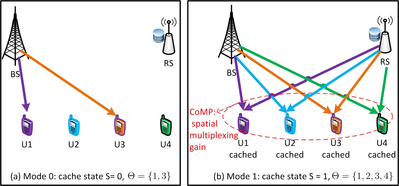
Figure 2: Illustration of cache-enabled opportunistic CoMP for a RAN with $M=2$.

As illustrated in Fig. 2, when $S=1$, there is spatial multiplexing gain due to cache-enabled CoMP transmission. The overall performance gain depends heavily on the probability of $S=1$. In the next section, we propose a novel MDS-coded random cache scheme which makes best use of the RS cache to increase $\textrm{Pr}\left[S=1\right]$.

II-C MDS-coded Random Cache

We use an example to show that, with a naive cache scheme, the CoMP opportunity ($S=1$) can be very small even if a significant portion of the video files are stored at the RS cache.

Example 1 (A Naive Cache Scheme).

Suppose that there are $L=2M=8$ video files with equal size of $F$ bits and the $k$-th video file is requested by the $k$-th user. The RS randomly stores half of the video packets (i.e., $0.5F$ bits) for each video file. The probability that the packets requested by a single user are in the RS cache is approximately 0.5. However, the probability of $S=1$ (i.e., the packets requested by all the $2M$ users are in the RS cache) is only $0.5^{2M}=0.0039$.

Hence, a more intelligent cache scheme is needed. In the following, we propose a novel MDS-coded random cache scheme which can significantly improve the probability of CoMP.

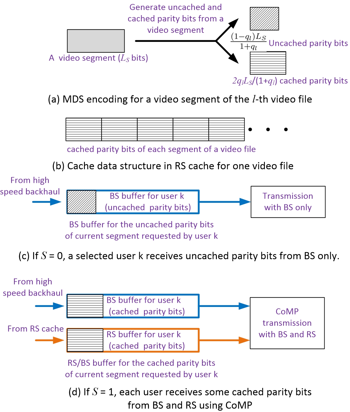
Figure 3: MDS-coded cache data structure and cache usage.

Cache Data Structure

Each video file is divided into segments. Each segment contains $L_{S}\gg\mu_{0}\tau$ bits and it is encoded into $L_{S}$ parity bits using an ideal MDS rateless code as illustrated in Fig. 3-(a), where $q_{l}\in\left[0,1\right]$ is called the cache control variable. An MDS rateless code generates an arbitrarily long sequence of parity bits from an information packet of $L_{S}$ bits, such that if the decoder obtains any $L_{S}$ parity bits, it can recover the original $L_{S}$ information bits. In practice, the MDS rateless code can be implemented using Raptor codes [14] at the cost of a small redundancy overhead. The RS stores $\frac{2q_{l}L_{S}}{1+q_{l}}$ parity bits for every segment of the $l$-th video file as illustrated in Fig. 3-(b). Such a cache data structure is more flexible than the naive cache scheme in Example 1 in the sense that we can control when to use the cached data.

Random Cache Usage

The cache usage is determined by the cache state $S$ as illustrated in Fig. 3-(c,d). If $S=1$, the BS and RS employ CoMP to jointly transmit the cached parity bits to the $2M$ users using the Mode 1 ZF scheme described in Section II-B. Otherwise, only $M$ users can be served by the BS using the Mode 0 ZF scheme. Using the above MDS-coded cache data structure, we can actively control the cache state $S$ for each time slot. The key to increasing the probability of CoMP in the system is to align the transmissions of the cached data for different users as much as possible. Specifically, for given cache control vector $\mathbf{q}=\left[q_{1},...,q_{L}\right]$ and $\pi$, let $q_{\textrm{min}}=\underset{1\leq k\leq 2M}{\textrm{min}}\left\{q_{\pi_{k}}\right\}$. Then the cache state $S$ at each time slot is independently generated according to a Bernoulli distribution with $\textrm{Pr}\left[S=1\right]=q_{\textrm{min}}$.

Remark 1 (Cache Underflow).

If $S=1$ and there is no untransmitted parity bits left in the RS cache for the segment requested by user $k$, a cache underflow event occurs for user $k$. Later in Proposition 1, we will show that the cache underflow probability tends to zero as the segment size $L_{S}\rightarrow\infty$. Hence, the effect of cache underflow is negligible for large $L_{S}$.

The following example illustrates the advantage of MDS-coded random cache scheme.

Example 2 (Advantage of MDS-coded random cache).

Consider the setup in Example 1. We have $q_{\pi_{k}}=0.5,\forall k$ and thus the probability of $S=1$ is $0.5$, which is much larger than that of the naive scheme in Example 1 ($0.0039$).

Compared with the naive caching scheme in Example 1, the probability of CoMP transmission ($S=1$) under the proposed MDS-coded random cache is $\textrm{min}_{k}\left\{q_{\pi_{k}}\right\}$ versus $\prod_{k=1}^{2M}q_{\pi_{k}}$. This represents a first order improvement in the opportunity of CoMP gain. Yet, there is a fundamental tradeoff between the performance gain and the RS cache size. Intuitively, the more popular the video file is, the larger portion of its parity bits should be stored in the RS cache to increase the CoMP probability. Hence, the value of $\mathbf{q}$ must be carefully controlled to achieve the best tradeoff among performance and required RS cache size. As such, the cache control variable is parameterized by the vector $\mathbf{q}=\left[q_{1},...,q_{L}\right]$.

II-D Queue Dynamics and QoS Metric

Each user maintains a queue for video playback as illustrated in Fig. 4. Let $Q_{k}\left(t\right)\in\mathcal{Q}$ denote the QSI (number of bits) of the playback buffer at the $k$-th user, where $\mathcal{Q}=\left[0,\infty\right)$ is the QSI state space. Let $\mathbf{Q}(t)=\left(Q_{1}\left(t\right),...,Q_{K}\left(t\right)\right)\in\boldsymbol{\mathcal{Q}}\triangleq\mathcal{Q}^{2M}$ denote the global QSI. The playback rate (departure rate) of user $k$ depends on the amount of video data in the playback buffer $Q_{k}(t)$ and is given by:

$$\mu_{k}\left(Q_{k}\left(t\right)\right)=\begin{cases}\frac{Q_{k}\left(t\right)\mu_{0}}{W_{L}},&Q_{k}\left(t\right)<W_{L},\\ \mu_{0},&Q_{k}\left(t\right)\geq W_{L},\end{cases}$$ (1)

where $W_{L}>\mu_{0}\tau$ is a parameter. If $Q_{k}\left(t\right)\geq W_{L}$, a constant playback rate $\mu_{0}$ (which is equal to the streaming rate) can be maintained. Otherwise, the playback rate is $\mu_{k}=\frac{Q_{k}\left(t\right)\mu_{0}}{W_{L}}$ to avoid buffer underflow. The dynamics of the playback buffer at user $k$ is given by

$$Q_{k}\left(t+1\right)=Q_{k}\left(t\right)+\left(r_{k}\left(g_{k}\left(t\right),p_{k}\left(t\right)\right)-\mu_{k}\left(Q_{k}\left(t\right)\right)\right)\tau.$$ (2)

Note that the playback rate in (1) ensures that $Q_{k}\left(t\right)\geq 0$.

Since the video playback quality of a user will be degraded whenever $Q_{k}<W_{L}$, we define the QoS requirement of each user in terms of the interruption probability:

$$I_{k}=\textrm{Pr}\left[Q_{k}<W_{L}\right].$$ (3)

We will elaborate more about the interruption cost together with other system costs in Section III-B.

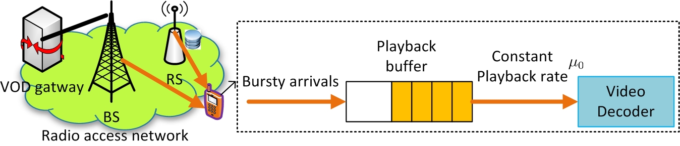
Figure 4: Playback buffer for video streaming at each user.

III Optimization Problem Formulation

In this section, we introduce the power control policy and formulate a two timescale optimization problem for video streaming under cache-enabled opportunistic CoMP. The control variables are partitioned into long-term and short-term control variables. As illustrated in Fig. 5, the long-term control variables (cache control variables $\mathbf{q}$) are adaptive to the distribution of the URP $\pi$ to induce CoMP opportunity. The short-term control variables (power control variables $\left\{p_{k},\forall k\right\}$) are adaptive to the instantaneous cache state $S$, CSI $\mathbf{H}$ and QSI $\mathbf{Q}$ to exploit the opportunistic CoMP gain and to guarantee the QoS requirements of the users for given $\mathbf{q}$ and $\pi$. The proposed two timescale control structure and the corresponding algorithm components are illustrated in Fig. 5. The ZF beamforming component and the random cache state generator have been discussed in Section II. The power control and cache control are two key algorithm components that will be respectively elaborated in Section IV and Section V. The other algorithm components and the overall solution will be discussed in Section VI.

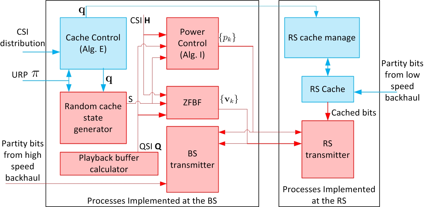
Figure 5: Summary of overall solution and the inter-relationship of the algorithm components. The blue / red blocks represent long timescale / short timescale processes. The blue / red arrows represent long-term / short-term signaling.

III-A Power Control Policy

Let $\boldsymbol{\chi}=\left(\mathbf{Q},S,\mathbf{H}\right)$ denote the global system state. At the beginning of each time slot, the BS determines the power control actions based on the global system state $\boldsymbol{\chi}$ according to the following stationary control policy.

Definition 1 (Stationary Power Control Policy).

A stationary power control policy for the $k$-th user $\Omega_{k}$ is a mapping from the global system state $\boldsymbol{\chi}$ to the power control actions of the $k$-th user. Specifically, we have $p_{k}=\Omega_{k}\left(\boldsymbol{\chi}\right)$. Furthermore, let $\Omega=\left\{\Omega_{k},\forall k\right\}$ denote the aggregation of the control policies for all the $2M$ users.

Given $\mathbf{q}$, $\pi$ and a control policy $\Omega$, the induced random process $\boldsymbol{\chi}\left(t\right)$ is a controlled Markov chain with the following transition probability:

$$\textrm{Pr}^{\left(\mathbf{q},\pi,\Omega\right)}\left[\boldsymbol{\chi}\left(t+1\right)\left|\boldsymbol{\chi}\left(t\right)\right.\right]=\;\;\;\;\;\;\;\;\;\;\;\;\;\;\;\;\;\;\;\;\;\;\;\;\;\;\;\;\;\;\;\;\;\;\;\;\;\;\;\;\;\;\;\;\;\;\;$$

$$\textrm{Pr}^{\left(\mathbf{q},\pi,\Omega\right)}\left[S\left(t+1\right)\right]\textrm{Pr}\left[\mathbf{H}\left(t+1\right)\right]\textrm{Pr}^{\left(\mathbf{q},\pi,\Omega\right)}\left[\mathbf{Q}\left(t+1\right)\left|\boldsymbol{\chi}\left(t\right)\right.\right],$$

where $\textrm{Pr}^{\left(\mathbf{q},\pi,\Omega\right)}$ means the probability w.r.t. the measure induced by the control policy $\Omega$ under given $\mathbf{q},\pi$; the queue transition probability is given by

$$\textrm{Pr}^{\left(\mathbf{q},\pi,\Omega\right)}\left[\mathbf{Q}\left(t+1\right)\left|\boldsymbol{\chi}\left(t\right)\right.\right]$$

$$= \begin{cases}1,&\textrm{if}\>Q_{k}\left(t+1\right),\forall k\>\textrm{is\>\ given\>\ by}\>(\ref{eq:Qdyn}),\\ 0,&\textrm{otherwise}.\end{cases}$$

The admissible control policy in this paper is defined as follows.

Definition 2 (Admissible Control Policy).

For given $\mathbf{q},\pi$, a policy $\Omega$ is admissible if the following requirements are satisfied:

1. $\Omega$ is a unichain policy, i.e., the controlled Markov chain $\boldsymbol{\chi}\left(t\right)$ under $\Omega$ has a single recurrent class (and possibly some transient states) [11].

2. The queueing system under $\Omega$ is stable in the sense that $\underset{T\rightarrow\infty}{\textrm{lim}}\textrm{E}^{\left(\mathbf{q},\pi,\Omega\right)}\left[\sum_{k=1}^{K}Q_{k}\left(T\right)\right]<\infty$, where $\textrm{E}^{\left(\mathbf{q},\pi,\Omega\right)}\left[\cdot\right]$ means taking expectation w.r.t. the probability measure induced by the control policy $\Omega$ under given $\mathbf{q},\pi$.

III-B Video Streaming Performance and Cost

For video streaming applications, there is a playback buffer at the users as illustrated in Fig. 4. The output of the playback buffer is the video decoding rate (playback rate) but the input of the buffer is random (randomness induced by the channel fading). During video streaming session, the user do not expect interruption in the playback process. However, playback interruption event occurs whenever the queue length of the playback buffer is less than $W_{L}$ as illustrated in Fig. 6. Hence, an important first order performance metric for video streaming is the probability of playback interruption. On the other hand, the playback buffer cost in the mobile must be explicitly accounted for. As a result, the system performance and cost are characterized by the interruption probability, the playback buffer overflow probability of the users (user centric performance metrics) and the average transmit power at the BS and RS (network centric performance metric).

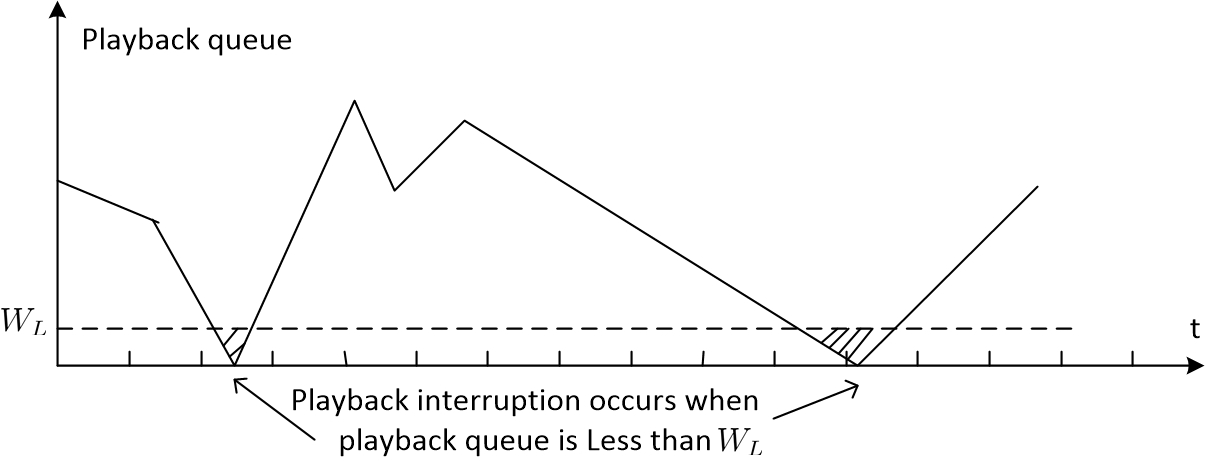
Figure 6: Illustration of the playback process and playback interruption at the user.

For given $\mathbf{q},\pi$ and an admissible control policy $\Omega$, the interruption probability and the playback buffer overflow probability of the $k$-th user are given by

$$I_{k}^{\left(\mathbf{q},\pi,\Omega\right)} = \underset{T\rightarrow\infty}{\textrm{lim sup}}\frac{1}{T}\sum_{t=1}^{T}\textrm{E}^{\left(\mathbf{q},\pi,\Omega\right)}\left[1\left(Q_{k}\left(t\right)<W_{L}\right)\right]$$ (4)

$$B_{k}^{\left(\mathbf{q},\pi,\Omega\right)} = \underset{T\rightarrow\infty}{\textrm{lim sup}}\frac{1}{T}\sum_{t=1}^{T}\textrm{E}^{\left(\mathbf{q},\pi,\Omega\right)}\left[1\left(Q_{k}\left(t\right)>W_{H}\right)\right]$$ (5)

where $W_{H}>W_{L}$ is the target maximum playback buffer size at the mobile. For technical reasons, we respectively use $e^{-\alpha\left(Q_{k}-W_{L}\right)^{+}}$ and $e^{-\alpha\left(W_{H}-Q_{k}\right)^{+}}$ as a smooth approximation of the indicator function in (4) and (5), where $\alpha>0$ is a smoothing parameter. As a result, the smooth approximation of the interruption probability and overflow probability is given by:

$$\overline{I}_{k}^{\left(\mathbf{q},\pi,\Omega\right)} = \underset{T\rightarrow\infty}{\textrm{lim sup}}\frac{1}{T}\sum_{t=1}^{T}\textrm{E}^{\left(\mathbf{q},\pi,\Omega\right)}\left[e^{-\alpha\left(Q_{k}\left(t\right)-W_{L}\right)^{+}}\right]$$ (6)

$$\overline{B_{k}}^{\left(\mathbf{q},\pi\Omega\right)} = \underset{T\rightarrow\infty}{\textrm{lim sup}}\frac{1}{T}\sum_{t=1}^{T}\textrm{E}^{\left(\mathbf{q},\pi,\Omega\right)}\left[e^{-\alpha\left(W_{H}-Q_{k}\left(t\right)\right)^{+}}\right]$$ (7)

It can be shown that the smooth approximation is tight ($\overline{I}_{k}^{\left(\mathbf{q},\pi,\Omega\right)}\rightarrow I_{k}^{\left(\mathbf{q},\pi,\Omega\right)}$ and $\overline{B_{k}}^{\left(\mathbf{q},\pi\Omega\right)}\rightarrow B_{k}^{\left(\mathbf{q},\pi,\Omega\right)}$) as $\alpha\rightarrow\infty$. The average total transmit power at the BS and RS is given by:

$$\overline{P}^{\left(\mathbf{q},\pi,\Omega\right)}=\underset{T\rightarrow\infty}{\textrm{lim sup}}\frac{1}{T}\sum_{t=1}^{T}\textrm{E}^{\left(\mathbf{q},\pi,\Omega\right)}\left[\sum_{k=1}^{2M}p_{k}\left(t\right)\right].$$

Note that the cost related to the RS is reflected in the average transmit power cost $\overline{P}^{\left(\mathbf{q},\pi,\Omega\right)}$, which is a summation of the average transmit power at the BS and the average transmit power at the RS. As a result, the final system cost is given by:

$$\overline{C}\left(\mathbf{q},\pi,\Omega\right)$$

$$= \sum_{k=1}^{2M}\left(\beta_{k}\overline{I}_{k}^{\left(\mathbf{q},\pi,\Omega\right)}+\gamma_{k}\overline{B_{k}}^{\left(\mathbf{q},\pi,\Omega\right)}\right)+\overline{P}^{\left(\mathbf{q},\pi,\Omega\right)}$$

$$= \underset{T\rightarrow\infty}{\textrm{lim sup}}\frac{1}{T}\sum_{t=1}^{T}\textrm{E}^{\left(\mathbf{q},\pi,\Omega\right)}\left[c\left(\mathbf{Q}\left(t\right),\Omega\left(\boldsymbol{\chi}\left(t\right)\right)\right)\right],$$

where $\beta_{k}>0$ and $\gamma_{k}>0$ are respectively the interruption price and buffer price of user $k$; $c\left(\mathbf{Q},\Omega\left(\boldsymbol{\chi}\right)\right)=\sum_{k=1}^{2M}\left(\hat{c}_{k}\left(Q_{k}\right)+p_{k}\right)$ with

$$\hat{c}_{k}\left(Q_{k}\right)=\beta_{k}e^{-\alpha\left(Q_{k}-W_{L}\right)^{+}}+\gamma_{k}e^{-\alpha\left(W_{H}-Q_{k}\right)^{+}}.$$ (8)

We have the following additional assumptions on $\beta_{k},\gamma_{k}$ and $\alpha$.

Assumption 3 (Assumptions on the Price Parameters $\left(\beta_{k},\gamma_{k}\right)$).

The parameters $\beta_{k},\gamma_{k}\forall k$ and $\alpha$ satisfy

$$e^{\left(W_{L}-W_{H}\right)\alpha}<\frac{\beta_{k}}{\gamma_{k}}<e^{\left(W_{H}-W_{L}\right)\alpha},\>\forall k,$$ (9)

$$\beta_{k}>\frac{\frac{1}{2}\left(\lambda_{0}e^{-\frac{1}{\lambda_{0}}}-E_{1}\left(\frac{1}{\lambda_{0}}\right)\right)+\gamma_{k}e^{-\frac{\left(W_{H}-W_{L}\right)\alpha}{2}}}{1-e^{-\frac{\left(W_{H}-W_{L}\right)\alpha}{2}}},$$ (10)

where $E_{1}\left(x\right)=\int_{x}^{\infty}\frac{e^{-t}}{t}dt$; $\lambda_{0}$ is the unique solution of $\frac{B_{W}}{2\textrm{ln}2}E_{1}\left(1/\lambda\right)=\mu_{0}$ w.r.t. $\lambda>0$.

If $\beta_{k}$ is too small, the power cost will dominate and the users will not be served at all (i.e., they are always allocated with zero power). The condition in (10) is used to avoid such an uninteresting degenerate case. Define

$$Q_{k}^{\circ}\triangleq\underset{Q_{k}}{\textrm{min}}\>\hat{c}_{k}\left(Q_{k}\right).$$ (11)

The condition in (9) is used to ensure that the per stage cost function $\hat{c}_{k}\left(Q_{k}\right)$ of user $k$ (excluding the power cost) attains the minimum at the queue length $Q_{k}^{\circ}\in\left(W_{L},W_{H}\right)$ which corresponds to the "desired" operating regime. Mathematically, Assumption 3 ensures that the solution of the approximated Bellman equation in Theorem 2 is valid. We also give an intuitive interpretation for the conditions in Assumption 3. Suppose that the queueing system $Q_{k}\left(t\right)$ is concentrated around $Q_{k}^{\Omega}$ under the control policy $\Omega$. Then the corresponding average arrival rate $\textrm{E}^{\left(\mathbf{q},\pi,\Omega\right)}\left[r_{k}\left(\mathbf{g}_{k},\Omega_{k}\left(\mathbf{Q},S,\mathbf{H}\right)\right)\right]\approx\mu_{k}\left(Q_{k}^{\Omega}\right)$. Hence the per user average cost under $\Omega$ can be approximated as $\hat{\overline{C}}_{k}\left(Q_{k}^{\Omega}\right)=\hat{c}_{k}\left(Q_{k}^{\Omega}\right)+\hat{\overline{P}}_{k}\left(Q_{k}^{\Omega}\right)$, where $\hat{\overline{P}}_{k}\left(Q_{k}^{\Omega}\right)$ is the average power required to support an average rate of $\mu_{k}\left(Q_{k}^{\Omega}\right)$. It follows from $\mu_{k}\left(Q_{k}\right)=\mu_{0},\forall Q_{k}\in\left[W_{L},\infty\right)$ that $\hat{\overline{C}}_{k}\left(Q_{k}^{\circ}\right)<\hat{\overline{C}}_{k}\left(Q_{k}\right),\forall Q_{k}\neq Q_{k}^{\circ}\in\left[W_{L},\infty\right)$. Hence the optimal control policy $\Omega^{*}$ that minimizes $\hat{\overline{C}}_{k}\left(Q_{k}^{\Omega}\right)$ either satisfies $Q_{k}^{\Omega^{*}}<W_{L}$ or $Q_{k}^{\Omega^{*}}=Q_{k}^{\circ}$. To avoid the uninteresting degenerate case where $Q_{k}^{\Omega^{*}}<W_{L}$, we require $\hat{\overline{C}}_{k}\left(Q_{k}\right)>\hat{\overline{C}}_{k}\left(Q_{k}^{\circ}\right),\forall Q_{k}\in\left[0,W_{L}\right]$. Using the fact that $\hat{\overline{C}}_{k}\left(Q_{k}\right)\geq\beta_{k},\forall Q_{k}\in\left[0,W_{L}\right]$, $\hat{c}_{k}\left(Q_{k}^{\circ}\right)\leq\hat{c}_{k}\left(\frac{W_{H}-W_{L}}{2}\right)$ and $\hat{\overline{P}}_{k}\left(Q_{k}^{\circ}\right)\leq\frac{\lambda_{0}e^{-\frac{1}{\lambda_{0}}}-E_{1}\left(\frac{1}{\lambda_{0}}\right)}{2}$ (this is because $\frac{\lambda_{0}e^{-\frac{1}{\lambda_{0}}}-E_{1}\left(\frac{1}{\lambda_{0}}\right)}{2}$ is the average power required to support an average rate of $\mu_{k}\left(Q_{k}^{\circ}\right)=\mu_{0}$ when $q_{\textrm{min}}=0$), it is easy to see that the condition in (10) ensures that $\hat{\overline{C}}_{k}\left(Q_{k}\right)>\hat{\overline{C}}_{k}\left(Q_{k}^{\circ}\right),\forall Q_{k}\in\left[0,W_{L}\right]$.

III-C Two timescale Optimization Formulation

The joint cache and power control problem is formulated as the following two timescale optimization problem:

$$\mathcal{P}:\>\underset{\mathbf{q}}{\textrm{min}}\>\textrm{E}\left[\underset{\Omega}{\textrm{min}}\>\overline{C}\left(\mathbf{q},\pi,\Omega\right)\right]+\eta\sum_{l=1}^{L}F_{l}q_{l},\>\textrm{s.t}.\>q_{l}\in\left[0,1\right],\forall l,$$

where the expectation is taken w.r.t. the distribution of $\pi$; the term $\sum_{l=1}^{L}F_{l}q_{l}$ represents the cache cost at the RS; and $\eta>0$ is the cache price.

Remark 2 (Interpretation of Pricing Vector).

The focus of the paper is to solve $\mathcal{P}$ for a given pricing vector $\left[\beta_{1},...,\beta_{2M},\gamma_{1},...,\gamma_{2M},\eta\right]$. In fact, the vector $\left[\beta_{1},...,\beta_{2M},\gamma_{1},...,\gamma_{2M},\eta\right]$ can be interpreted as the pricing vectors or the Lagrange Multipliers (LM).

• Pricing Vector Interpretation: In practice, a Pareto optimal solution from the knee region of the Pareto front is usually more preferable than other solutions [15]. Once we can solve problem $\mathcal{P}$ (for a given pricing vector), there are existing algorithms (such as multi-objective evolutionary algorithm (MOEA) [15, 16]) that can be used to determine the appropriate pricing vector to achieve the knee solutions.

• LM Vector Interpretation: In practice, we usually have a constraint on the RS cache size. The cache price $\eta$ can be interpreted as the Lagrange multiplier associated with the RS cache size constraint. Similarly, the prices $\beta_{k}$ and $\gamma_{k}$ can be interpreted as the Lagrange multipliers associated with the constraints on interruption probability and playback buffer overflow probability requirements for the $k$-th video streaming user.

Using primal decomposition [17], problem $\mathcal{P}$ can be decomposed into two subproblems.

Inner MDP Subproblem (Short-term Power Control): Optimization of $\Omega$ for given $\mathbf{q},\pi$.

$$\mathcal{P}_{I}\left(\mathbf{q},\pi\right):\>\overline{C}^{*}\left(\mathbf{q},\pi\right)\triangleq\underset{\Omega}{\textrm{min}}\>\overline{C}\left(\mathbf{q},\pi,\Omega\right).$$

Outer Caching Subproblem (Long-term Cache Control): Optimization of $\mathbf{q}$.

$$\mathcal{P}_{O}:\>\underset{\mathbf{q}}{\textrm{min}}\>\textrm{E}\left[\overline{C}^{*}\left(\mathbf{q},\pi\right)\right]+\eta\sum_{l=1}^{L}F_{l}q_{l},\>\textrm{s.t}.\>q_{l}\in\left[0,1\right],\forall l.$$

Subproblem $\mathcal{P}_{I}\left(\mathbf{q},\pi\right)$ belongs to the infinite horizon average cost MDP, and it is well known that there is no simple solution associated with such MDP. Brute force value iterations or policy iterations [11] could not lead to any viable solutions due to the curse of dimensionality. Subproblem $\mathcal{P}_{O}$ is also a difficult stochastic optimization problem. The term $\overline{C}^{*}\left(\mathbf{q},\pi\right)$ in the objective function depends on the optimal solution of the inner MDP problem and there is no closed form characterization. Moreover, the distribution of $\pi$ is unknown and we cannot calculate the expectation $\textrm{E}\left[\overline{C}^{*}\left(\mathbf{q},\pi\right)\right]$ explicitly. In Section IV, by exploiting the special structure in our problem, we derive an approximate Bellman equation to obtain a low complexity solution for the inner MDP problem $\mathcal{P}_{I}\left(\mathbf{q},\pi\right)$. In Section V, we derive a closed form convex approximation of $\overline{C}^{*}\left(\mathbf{q},\pi\right)$, which is the key to develop a robust stochastic subgradient algorithm to find an asymptotically optimal solution for $\mathcal{P}_{O}$.

IV Low Complexity Power Control Solution for $\mathcal{P}_{I}\left(\mathbf{q},\pi\right)$

To simplify notation, we use $\textrm{E}\left[\cdot\right]$ to denote $\textrm{E}^{\left(\mathbf{q},\pi,\Omega\right)}\left[\cdot\right]$, and $\textrm{Pr}\left[\cdot|\Omega\right]$ to denote $\textrm{Pr}^{\left(\mathbf{q},\pi,\Omega\right)}\left[\cdot\right]$ in this section.

IV-A Optimality Conditions and Approximate Bellman Equation

Utilizing the i.i.d. property of $\left\{S,\mathbf{H}\right\}$ w.r.t. time slots, the following gives the optimality condition of problem $\mathcal{P}_{I}\left(\mathbf{q},\pi\right)$.

Theorem 1 (Sufficient Optimality Conditions for $\mathcal{P}_{I}\left(\mathbf{q},\pi\right)$).

For given $\mathbf{q},\pi$, assume there exists a $\left(\theta^{*},\left\{V^{*}\left(\mathbf{Q}\right)\right\}\right)$ that solves the following equivalent Bellman equation:

$$\theta^{*}\tau+V^{*}\left(\mathbf{Q}\right) = \textrm{E}\bigg{[}\underset{\left\{p_{k}\right\}}{\textrm{min}}\bigg{[}c\left(\mathbf{Q},\left\{p_{k}\right\}\right)\tau+$$ (12)

$$\sum_{\mathbf{Q}^{{}^{\prime}}}\textrm{Pr}\left[\mathbf{Q}^{{}^{\prime}}|\boldsymbol{\chi},\left\{p_{k}\right\}\right]V^{*}\left(\mathbf{Q}^{{}^{\prime}}\right)\bigg{]}\bigg{|}\mathbf{Q}\bigg{]}$$

$$\forall\mathbf{Q}\in\boldsymbol{\mathcal{Q}},$$

Furthermore, for all admissible control policy $\Omega$ and initial queue state $\mathbf{Q}\left(0\right)$, $V^{*}$ satisfies the following transversality condition:

$$\underset{T\rightarrow\infty}{\textrm{lim sup}}\frac{1}{T}\textrm{E}\left[\left.V^{*}\left(\mathbf{Q}\left(T\right)\right)\right|\mathbf{Q}\left(0\right)\right]=0.$$ (13)

Then, $\theta^{*}=\overline{C}^{*}\left(\mathbf{q},\pi\right)$ is the optimal average cost and $V^{*}\left(\mathbf{Q}\right)$ is called the relative value function. If $\left\{p_{k}^{*}\right\}$ attains the minimum of the R.H.S. of (12) for given $\boldsymbol{\chi}$, then $\Omega^{*}\left(\boldsymbol{\chi}\right)=\left\{p_{k}^{*}\right\}$ is the optimal control policy for Problem $\mathcal{P}_{I}\left(\mathbf{q},\pi\right)$.

Please refer to Appendix -A for the proof.

Note that the solution given by Theorem 1 is unique due to the unichain assumption of the control policy [11].

Using Taylor expansion, we establish the following corollary on the approximation of the Bellman equation in (12).

Corollary 1 (Approximate Bellman Equation).

For any given $\mathbf{q},\pi$, if

1. there is a unique $\left(\theta^{*},\left\{V^{*}\left(\mathbf{Q}\right)\right\}\right)$ that satisfies the equivalent Bellman equation (12) and transversality condition (13) in Theorem 1.

2. there exist $\theta$ and $V\left(\mathbf{Q}\right)\in\mathcal{C}^{1}\left(\mathbb{R}_{+}^{2M}\right)$ that solve the following approximate Bellman equation:

   $$\theta=\textrm{E}\bigg{[}\underset{\left\{p_{k}\right\}}{\textrm{min}}\bigg{[}c\left(\mathbf{Q},\left\{p_{k}\right\}\right)+\sum_{k=1}^{2M}\frac{\partial V\left(\mathbf{Q}\right)}{\partial Q_{k}}\;\;\;\;\;\;\;\;\;\;\;\;\;\;$$

   $$\left.\times\left(r_{k}\left(\mathbf{g}_{k},p_{k}\right)-\mu_{k}\left(Q_{k}\right)\right)\bigg{]}\right|\mathbf{Q}\bigg{]},$$ (14)

   for all $\mathbf{Q}\in\boldsymbol{\mathcal{Q}}$. Furthermore, for all admissible control policy $\Omega$ and initial queue state $\mathbf{Q}(0)$, the transversality condition in (13) is satisfied for $V$.

Then we have

$$\theta^{*} = \theta+o\left(1\right)$$

$$V^{*}\left(\mathbf{Q}\right) = V\left(\mathbf{Q}\right)+o\left(1\right),\>\forall\mathbf{Q}\in\boldsymbol{\mathcal{Q}},$$

where the error term $o(1)$ asymptotically goes to zero for sufficiently small slot duration $\tau$.

Please refer to Appendix -B for the proof.

By Corollary 1, the solution of the Bellman equation (12) can be approximated by the solution of the approximate Bellman equation in (14), and the approximation is asymptotically accurate as $\tau\rightarrow 0$. However, solving the approximate Bellman equation still involves solving a large system of nonlinear fixed point equations. In the following subsection, we exploit the specific structure of our problem to derive a simple solution for the approximate Bellman equation.

IV-B Solution for the Approximate Bellman Equation

In the proposed opportunistic CoMP scheme, the interference among users is completely eliminated by ZF beamforming. As a result, the dynamics of the playback buffer at the $2M$ users are decoupled and we can obtain a closed form solution for the approximate Bellman equation by solving a set of independent single-variable non-linear equations as elaborated below.

We first derive the distribution of the effective channel $g_{k}$ for given $\mathbf{q}$ and $\pi$.

Lemma 1 (PDF of the Effective Channel).

For given $\mathbf{q}$ and $\pi$, the PDF of $g_{k}$ is given by

$$h_{g_{k}}\left(x\right) = \left(\frac{1+q_{\textrm{min}}}{2}\right)e^{-x}+\left(\frac{1-q_{\textrm{min}}}{2}\right)\delta\left(x\right),$$

where $q_{\textrm{min}}=\underset{1\leq k\leq K}{\textrm{min}}\left\{q_{\pi_{k}}\right\}$; and $\delta(\cdot)$ denote the Dirac delta function.

Please refer to Appendix -C for the proof.

Recall the definition of $Q_{k}^{\circ}$ in (11). Note that under Assumption 3, we have

$$Q_{k}^{\circ}=\frac{\textrm{log}\beta_{k}-\textrm{log}\gamma_{k}}{2\alpha}+\frac{W_{L}+W_{H}}{2}\in\left(W_{L},W_{H}\right).$$ (15)

Let $\tilde{\lambda}_{k}\left(x\right)$ denote the unique solution of the equation

$$\frac{B_{W}\left(1+q_{\textrm{min}}\right)}{2\textrm{ln}2}E_{1}\left(-\frac{\textrm{ln}2}{\lambda B_{W}}\right)-\mu_{k}\left(x\right)=0,$$ (16)

w.r.t. $\lambda\in\mathbb{R}_{-}$ for any $x\in\mathcal{Q}$. Then the following theorem holds.

Theorem 2 (Closed-Form Solution of (14)).

For any $1\leq k\leq 2M$, let

$$\tilde{\theta}_{k} = \hat{c}_{k}\left(Q_{k}^{\circ}\right)-\frac{\left(1+q_{\textrm{min}}\right)}{2}$$

$$\times\left(\frac{\tilde{\lambda}_{k}\left(Q_{k}^{\circ}\right)B_{W}}{\textrm{ln}2}e^{\frac{\textrm{ln}2}{\tilde{\lambda}_{k}\left(Q_{k}^{\circ}\right)B_{W}}}+E_{1}\left(-\frac{\textrm{ln}2}{\tilde{\lambda}_{k}\left(Q_{k}^{\circ}\right)B_{W}}\right)\right),$$

and consider the following set of independent nonlinear equations w.r.t. $f_{k}$ for all $x\in\mathcal{Q}$:

$$\hat{c}_{k}\left(x\right)+\left(\frac{B_{W}\left(1+q_{\textrm{min}}\right)}{2\textrm{ln}2}E_{1}\left(-\frac{\textrm{ln}2}{f_{k}B_{W}}\right)-\mu_{k}\left(x\right)\right)f_{k}$$ (18)

$$-\frac{\left(1+q_{\textrm{min}}\right)}{2}\left(\frac{f_{k}B_{W}}{\textrm{ln}2}e^{\frac{\textrm{ln}2}{f_{k}B_{W}}}+E_{1}\left(-\frac{\textrm{ln}2}{f_{k}B_{W}}\right)\right) = \tilde{\theta}_{k}.$$

Then the following are true:

1. For $x\in\left[0,Q_{k}^{\circ}\right]$, (18) has a unique solution denoted by $\tilde{f}_{k}\left(x\right),\>x\in\left[0,Q_{k}^{\circ}\right]$ over the region $f_{k}\in\left(-\infty,\tilde{\lambda}_{k}\left(x\right)\right]$.

2. For $x\in\left(Q_{k}^{\circ},\infty\right)$, (18) has a unique solution denoted by $\tilde{f}_{k}\left(x\right),\>x\in\left(Q_{k}^{\circ},\infty\right)$ over the region $f_{k}\in\left[\tilde{\lambda}_{k}\left(x\right),\infty\right]$.

3. $\tilde{\theta}\triangleq\sum_{k=1}^{2M}\tilde{\theta}_{k}$ and $\tilde{V}\left(\mathbf{Q}\right)\triangleq\sum_{k=1}^{2M}\int_{Q_{k}^{\circ}}^{Q_{k}}\tilde{f}_{k}\left(x\right)dx,\>\forall\mathbf{Q}\in\boldsymbol{\mathcal{Q}}$ satisfy the approximate Bellman equation (14). Moreover, $\tilde{V}\left(\mathbf{Q}\right)$ satisfies the transversality condition in (13) and thus $\theta^{*}=\tilde{\theta}+o\left(1\right)$ and $V^{*}\left(\mathbf{Q}\right)=\tilde{V}\left(\mathbf{Q}\right)+o\left(1\right),\>\forall\mathbf{Q}\in\boldsymbol{\mathscr{Q}}$, where $\theta^{*}$ is the optimal average cost and $V^{*}\left(\mathbf{Q}\right)$ is the optimal value function as defined in Corollary 1.

Please refer to Appendix -D for the proof.

Based on the closed form solution for the approximate Bellman equation in Theorem 2, the power control solution for given QSI $\mathbf{Q}$, cache state $S$ and CSI $\mathbf{H}$ is

$$p_{k}=\left(-\frac{\tilde{f}_{k}\left(Q_{k}\right)B_{W}}{\textrm{ln}2}-\frac{1}{g_{k}}\right)^{+},\forall k.$$ (19)

Note that the power control solution in (19) only requires the partial derivatives of the approximate value function $\frac{\partial\tilde{V}\left(\mathbf{Q}\right)}{\partial Q_{k}}\triangleq\tilde{f}_{k}\left(Q_{k}\right),\forall k$, which can be easily found by solving (18) in Theorem 2. The solution in (19) has a multi-level water-filling structure, where the water level depends on the QSI via $\tilde{f}_{k}\left(Q_{k}\right)$, which captures the urgency of the $k$-th data flow. The overall power control algorithm is summarized in Table I. By Theorem 2, the proposed power control algorithm is asymptotically optimal as $\tau\rightarrow 0$. Furthermore, the cache underflow probability under the proposed power control is negligible for large $L_{S}$ as proved in the following proposition.

Proposition 1 (Cache Underflow for Large $L_{S}$).

For given $\mathbf{q},\pi$ and under the power control policy in Table I, the cache underflow probability tends to zero as the segment size $L_{S}\rightarrow\infty$.

Please refer to Appendix -E for the proof.

Table I: Algorithm I (Power control for Problem $\mathcal{P}_{I}\left(\mathbf{q},\pi\right))$

Actions at the beginning of each time slot:

1: Calculate $\tilde{f}_{k}\left(Q_{k}\right),\forall k$ by solving (18) with current $\mathbf{Q}$.

2: Obtain the transmit powers using (19) with current $g_{k},\forall k$.

V Asymptotically Optimal Solution for $\mathcal{P}_{O}$

One challenge of solving $\mathcal{P}_{O}$ is that the objective function depends on the optimal average cost $\overline{C}^{*}\left(\mathbf{q},\pi\right)$ of the inner MDP problem, which is difficult to obtain. To tackle this difficulty, we derive an asymptotically accurate closed form approximation for $\overline{C}^{*}\left(\mathbf{q},\pi\right)$.

Theorem 3 (Asymptotic Approximation of $\overline{C}^{*}\left(\mathbf{q},\pi\right)$).

As $\frac{\mu_{0}}{B_{W}}\rightarrow\infty$ and $\tau\rightarrow 0$, we have

$$\frac{\left|\overline{C}^{*}\left(\mathbf{q},\pi\right)-\hat{C}\left(\mathbf{q},\pi\right)\right|}{\overline{C}^{*}\left(\mathbf{q},\pi\right)}=\mathcal{O}\left(\frac{\mu_{0}}{B_{W}}e^{-\frac{\mu_{0}}{B_{W}}}\right)\rightarrow 0,$$

where

$$\hat{C}\left(\mathbf{q},\pi\right)=\sum_{k=1}^{2M}\left(\xi e^{-a_{1}+\frac{\mu_{0}\textrm{ln}2}{B_{W}\xi}}-(a_{2}+e)\xi+e+\hat{c}_{k}\left(Q_{k}^{\circ}\right)\right),$$

where $\xi=\frac{1+\underset{1\leq k\leq 2M}{\textrm{min}}\left\{q_{\pi_{k}}\right\}}{2}$; $a_{1}=\textrm{log}\left(e^{-\frac{\mu_{0}\textrm{ln}2}{B_{W}}}\right)e^{-e^{-\frac{\mu_{0}\textrm{ln}2}{B_{W}}}}+E_{1}\left(e^{-\frac{\mu_{0}\textrm{ln}2}{B_{W}}}\right)$ and $a_{2}=E_{1}\left(e^{-\frac{\mu_{0}\textrm{ln}2}{B_{W}}}\right)$; $\hat{c}_{k}\left(\cdot\right)$ and $Q_{k}^{\circ}$ are given in (8) and (15) respectively.

Please refer to Appendix -F for the proof.

Then the following corollary follows immediately from Theorem 3.

Corollary 2 (Asymptotic equivalence of $\mathcal{P}_{O}$).

Let $\tilde{\mathbf{q}}$ be an optimal solution of the problem

$$\mathcal{P}_{E}:\>\underset{\mathbf{q}}{\textrm{min}}\>U\left(\mathbf{q}\right),\>\textrm{s.t}.\>q_{l}\in\left[0,1\right],\forall l,$$

where $U\left(\mathbf{q}\right)=\textrm{E}\left[\hat{C}\left(\mathbf{q},\pi\right)\right]+\eta\sum_{l=1}^{L}F_{l}q_{l}$. Let $C^{*}$ be the optimal value of $\mathcal{P}_{O}$. Then we have

$$\left|\textrm{E}\left[\overline{C}^{*}\left(\tilde{\mathbf{q}},\pi\right)\right]+\eta\sum_{l=1}^{L}F_{l}\tilde{q}_{l}-C^{*}\right|/C^{*} \rightarrow 0,$$ (20)

as $\frac{\mu_{0}}{B_{W}}\rightarrow\infty$ and $\tau\rightarrow 0$.

By Corollary 2, the solution of $\mathcal{P}_{O}$ can be approximated by the solution of $\mathcal{P}_{E}$, and the approximation is asymptotically accurate for high SNR and small slot size $\tau$. It can be shown that $\xi$ is a concave function w.r.t. $\mathbf{q}$ and $\hat{C}\left(\mathbf{q},\pi\right)$ is decreasing with $\xi$ for $q_{l}\in\left[0,1\right],\forall l$. Using the vector composition rule for convex function [18], $\hat{C}\left(\mathbf{q},\pi\right)$ is convex w.r.t. $\mathbf{q}$ and thus $\mathcal{P}_{E}$ is also a convex problem. Hence, we propose a stochastic subgradient algorithm which is able to converge to the optimal solution of $\mathcal{P}_{E}$ without knowing the distribution of $\pi$. The algorithm is summarized in Table II and the global convergence is established in the following Theorem.

Theorem 4 (Convergence of Algorithm E).

If the step sizes $\sigma^{(i)}>0$ in Algorithm E satisfies: 1) $\sum_{i=1}^{\infty}\left(\sigma^{(i)}\right)^{2}<\infty$; 2) $\sum_{i=1}^{\infty}\sigma^{(i)}=\infty$, then Algorithm E converges to an optimal solution $\tilde{\mathbf{q}}$ of Problem $\mathcal{P}_{E}$ with probability 1.

The convergence proof follows directly from [19, Theorem 3.3].

Table II: Algorithm E (for Solving Problem $\mathcal{P}_{E}$)

Initialization: Choose initial $\mathbf{q}$: $q_{l}\in\left[0,1\right],\forall l$. Let $i=1$.

Step 1: Calculate a noisy unbiased subgradient of $U\left(\mathbf{q}\right)$,

$\hat{\nabla}U=\left[\widehat{\frac{\partial U}{\partial q_{1}}},...,\widehat{\frac{\partial U}{\partial q_{L}}}\right]^{T}$ based on current $\mathbf{q},\pi$:

$\widehat{\frac{\partial U}{\partial q_{l}}}=$

$M\left[\left(1-\frac{\mu_{0}\textrm{ln}2}{B_{W}\xi}\right)e^{-a_{1}+\frac{\mu_{0}\textrm{ln}2}{B_{W}\xi}}-a_{2}-e\right]1\left(l=\pi_{k^{*}}\right)+\eta F_{l},\forall l,$

where $k^{*}$ is any index satisfying $q_{\pi_{k^{*}}}=\underset{1\leq k\leq 2M}{\textrm{min}}\left\{q_{\pi_{k}}\right\}$.

Step 2: Choose proper step size $\sigma^{(i)}>0$ and update $\mathbf{q}$ as

$q_{l}=\textrm{min}\left(\left(q_{l}-\sigma^{(i)}\widehat{\frac{\partial U}{\partial q_{l}}}\right)^{+},1\right),\forall l$

Step 3: Let $i=i+1$. When $\pi$ is changed, return to Step 1.

VI Implementation Considerations

VI-A Summary of the Overall Solution

Fig. 5 summarizes the overall solution and the inter-relationship of the algorithm components. The solutions are divided into long timescale process and short timescale process. The long timescale processing consists of Algorithm E (cache control) and RS cache management. The short timescale processing consists of random cache state generator, ZF beamforming and Algorithm I (power control). The power control and cache control processes are implemented at the BS, while the cache management process is implemented at the RS. Whenever the URP $\pi$ changes, the updated cache control vector $\mathbf{q}$ is computed from the BS and pass to the RS. Then the RS cache management updates the RS cache according to $\mathbf{q}$. Specifically, if the cached parity bits for each segment of the $l$-th video file is less than $\frac{2q_{l}L_{S}}{1+q_{l}}$ bits, it will request new parity bits from the low speed wireless backhaul. Otherwise, it will drop some cached parity bits. At each time slot, the cache state $S$ is generated from the random cache state generator using $\mathbf{q}$ and $\pi$, the QSI $\mathbf{Q}$ is calculated at the BS according to the queue dynamics in (2), and the CSI $\mathbf{H}$ is obtained via feedback from the users. Furthermore, at each time slot, the power control and ZF beamforming vectors are determined at the BS based on the CSI $\mathbf{H}$, QSI $\mathbf{Q}$ and cache state $S$. If $S=1$, they are sent to the RS for opportunistic CoMP transmission.

VI-B Computational Complexity

The main computation complexity of the proposed solution is dominated by three algorithm components, namely, the ZF beamforming, the power control Algorithm I and the long term cache control Algorithm E. We analyze the complexity of each algorithm component as follows.

• Complexity of ZF beamforming: At each time slot, the calculation of the ZF beamforming vectors $\overline{\mathbf{v}}_{k},\forall k\in\Theta$ (if $S=0$) requires a $M\times M$ matrix inversion and the calculation of the ZF beamforming vectors $\mathbf{v}_{k},\forall k$ (if $S=1$) requires a $2M\times 2M$ matrix inversion. The complexity of ZF beamforming is polynomial w.r.t. the number of antennas $M$ at the BS/RS.

• Complexity of the power control Algorithm I: At each time slot, we need to calculate $\tilde{f}_{k}\left(Q_{k}\right),\forall k$ by solving $2M$ independent single-variable nonlinear equations as in (18). Then the power control is calculated using the multi-level water-filling solution in (19), which only involves several floating point operations (FLOPs). Hence, the complexity of Algorithm I only increases linearly with the number of users $2M$.

• Complexity of the long term cache control Algorithm E: For each realization of $\pi$, we need to calculate the noisy unbiased subgradient $\hat{\nabla}U$ of $U\left(\mathbf{q}\right)$. The subgradient $\hat{\nabla}U$ has $L$ elements and the calculation of each element $\widehat{\frac{\partial U}{\partial q_{l}}}$ only requires several FLOPs. Then the cache control vector $\mathbf{q}$ is updated using a simple subgradient method. Hence, the complexity of Algorithm E only increases linearly with the number of video files $L$. Moreover, the above subgradient update is performed at a much slower time scale compared to the time slot rate.

In summary, using the closed-form approximation of $V^{*}\left(\mathbf{Q}\right)$ in Theorem 2, the proposed solution only has polynomial complexity w.r.t. the number of antennas $M$ at the BS/RS, and linearly complexity w.r.t. the number of users $2M$ and the number of video files $L$. The complexity is very low compared with brute-force value iteration [11] which has exponential complexity w.r.t. $2M$. Table III illustrates a comparison on the matlab computational time among the brute force MDP, the baselines defined in Section VII and the proposed solution. It can be seen that the per time slot computation time of the proposed solution is similar to the simple baselines without RS and is much lower than the decode and forward (DF) relay scheme in [20] or the brute-force value iteration [11]. This shows that the proposed solution is suitable for video streaming applications that requires real-time processing.

Table III: Comparison of the MATLAB computational time of the proposed scheme and the baselines in one time slot. The simulation setup is given in Section VII.

	$M=2$	$M=4$	$M=8$
Proposed	0.45ms	0.83ms	1.67ms
Baseline 1,2 (without RS)	0.13ms	0.21ms	0.44ms
Baseline 3 (Q-weighted DF)	2.12ms	4.56ms	10.42ms
Brute-Force Value Iteration	879s	$>10^{4}$s	$>10^{4}$s

VI-C Signaling Overheads

The short term signaling overhead is small compared to the conventional CoMP schemes [1, 2]. At each time slot, the BS first broadcasts the cache state $S$ and the user selection set $\Theta$ to the users. Then each selected user $k$ feedbacks its channel vector $\overline{\mathbf{h}}_{k}$ (if $S=0$) or $\mathbf{h}_{k}$ (if $S=1$) to the BS. Finally, if $S=1$, the BS sends the power allocation $\left\{p_{k},\forall k\right\}$ and the beamforming vectors $\left\{\mathbf{v}_{k},\forall k\right\}$ to the RS. The above signaling overhead is similar to the conventional closed-loop multi-user MIMO systems [21] and can be supported by the modern wireless systems such as LTE [22]. The long term cache control signaling between the BS and RS is very small since $\mathbf{q}$ is only sent to the RS once for each realization of $\pi$. For the cache update process, whenever $q_{l}$ is increased, the RS needs to request new parity bits from the wireless backhaul. Since $\mathbf{q}$ is adaptive to the distribution of $\pi$ and it changes very slowly, the wireless backhaul is enough to support the cache update process. Table. IV illustrates the cache update loading (in terms of the average wireless backhaul throughput used for cache update) versus different RS cache occupancy (i.e., the total size of the cached data at RS). The corresponding SNR gain over the baselines in Section VII (when achieving the same interruption probability $10^{-3}$) is also illustrated.

Table IV: Cache update loading under different RS cache occupancy and SNR gains. We assume that the popularity of the video files (i.e., the distribution of $\pi$) changes every week. The system setup is given in Section VII. As a comparison, if conventional CoMP [2] is employed, the backhaul loading between the BS and RS for exchanging the payload data is $8$Mbps.

RS cache	Cache update	SNR gain over	SNR gain over
occupancy	loading	Baseline 2	baseline 3
1.8G Bytes	25Kbps	4.9dB	3.8dB
1.3G Bytes	18Kbps	3.7dB	2.6dB
0.9G Bytes	12Kbps	2.6dB	1.5dB

VII Simulation Results

Consider a video streaming system with $L=6$ video files and $2M=4$ users. The size of each video file is $600$M Bytes and the streaming rate is $2$M bits/s. Both the BS and RS are equipped with $M=2$ antennas. Assume that each user independently accesses the $l$-th video file with probability $\rho_{l}$, and we set $\boldsymbol{\rho}=\left[\rho_{1},...,\rho_{6}\right]=\left[0.6,0.3,0.08,0.01,0.005,0.005\right]$, which represents the popularity of different video files. Note that $\boldsymbol{\rho}$ is only used to generate the realizations of URP $\pi$ and the control algorithms do not have the knowledge of $\boldsymbol{\rho}$. The other system parameters are set as

$$B_{W}=1\textrm{MHz}, \tau=5\textrm{ms}, \alpha=7.5\times 10^{-5},$$

$$W_{H}=2.5\times 10^{5}\textrm{bits}, W_{L}=2\times 10^{4}\textrm{bits}.$$

VII-A Convergence of the Cache Control Algorithm E

In Fig. 7, we plot the objective value $U\left(\mathbf{q}\right)$ of $\mathcal{P}_{E}$ versus the number of realizations of $\pi$ (i.e., the number of iterations of Algorithm E) for different cache prices $\eta$. We fix $\beta_{k}=\gamma_{k}=15,\>\forall k$. The corresponding RS cache occupancy is also given besides each convergence curve. It can be seen that Algorithm $E$ quickly converges.

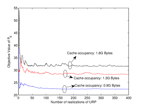
Figure 7: Convergence of Algorithm E

VII-B Performance Gain of the Proposed Solution w.r.t. Baselines

The following baselines are considered.

Baseline 1 (CSI-only without RS): There is no RS. The physical layer reduces to the Mode 0 ZF scheme in Section II-B. The power control is only adaptive to the CSI. Specifically, at each time slot, the power control is obtained by solving the following optimization problem:

$$\underset{\left\{p_{k}\right\}}{\textrm{max}}\>\sum_{k\in\Theta}r_{k}^{BL1}-\kappa\sum_{k\in\Theta}p_{k},$$

where $r_{k}^{BL1}$ is the instantaneous data rate of user $k$ under baseline 1; and $\kappa>0$ is used to tradeoff between interruption probability and average transmit power.

Baseline 2 (Q-weighted without RS): The physical layer is the same as that in baseline 1. The power control is adaptive to both CSI and QSI. Specifically, at each time slot, the power control is obtained by solving the following optimization problem:

$$\underset{\left\{p_{k}\right\}}{\textrm{max}}\>\sum_{k\in\Theta}\left(W_{H}-Q_{k}\right)^{+}r_{k}^{BL1}-\kappa\sum_{k\in\Theta}p_{k}.$$ (21)

Baseline 3: (Q-weighted DF): At each time slot, $2$ users are selected randomly for transmission from the $4$ users. Then the full decode and forward (DF) relay scheme proposed in [20] is employed at the physical layer to serve the selected $2$ users. The channel between the BS and RS is modeled by $\mathbf{H}_{BR}=10\mathbf{H}_{W}\in\mathbb{C}^{M\times M}$, where $\mathbf{H}_{W}$ has i.i.d. complex Gaussian entries of zero mean and unit variance (i.e., the path gain of the the channel between the BS and RS is 20dB larger than the user channel $\mathbf{h}_{k}$’s). In the relay listening phase, the interference among the data streams of different users is eliminated using ZF transmit beamforming at the BS and ZF receiving beamforming at the RS. In the BS-RS cooperative transmission phase, the multi-user interference is eliminated using joint ZF beamforming at the BS and RS. At each time slot, the power control is obtained by solving the optimization problem in (21) with $r_{k}^{BL1}$ replaced by $r_{k}^{BL3}$, the instantaneous data rate of user $k$ under baseline 3.

In the simulations, we let $\beta_{k}=\gamma_{k}=\beta,\forall k$ and vary $\beta,\eta$ to obtain different tradeoff curves. For the baselines, the tradeoff curves are obtained by varying $\kappa$. In Fig. 8 and 9, we respectively plot the playback interruption probability and playback buffer overflow probability of user $k$ versus the average per-user transmit power $\textrm{E}\left[p_{k}\right]$. It can be observed that the proposed solution has a significant performance gain over all baselines, and the gain increases as more parity bits of the video files are stored in the RS cache. As the average transmit power increases, both the interruption probability and the playback buffer overflow probability of the proposed solution decreases; however, the playback buffer overflow probability of the baselines increases. This shows that the system cost function and the associated power control algorithm must be carefully designed in order to achieve a good tradeoff between interruption probability, playback buffer overflow probability and the transmit power cost. For example, in Fig. 8, although the interruption probability of the baselines approaches that of the proposed solution as the average transmit power becomes large, the corresponding playback buffer overflow probability is also very large. In Fig. 9, although the playback buffer overflow probability of the baselines is small for small average transmit power, the corresponding interruption probability is very large. As a result, the overall combined video streaming performance of the baselines is much worse than the proposed solution as illustrated in Fig. 10. This demonstrates that the proposed solution can achieve a much better tradeoff between different system costs.

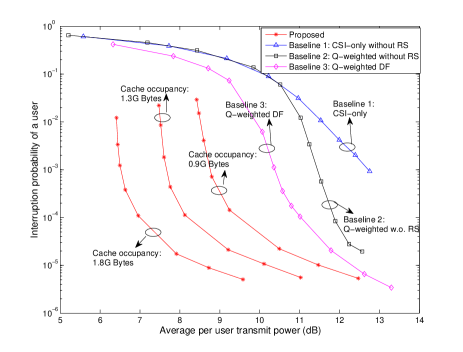
Figure 8: Playback interruption probability versus the average per-user transmit power.

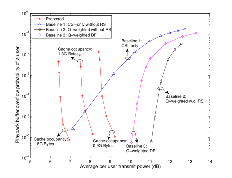
Figure 9: Playback overflow probability versus the average per-user transmit power.

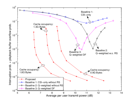
Figure 10: Combined interruption probability and playback overflow probability versus the average per-user transmit power.

VIII Conclusion

We introduce a cache-enabled opportunistic CoMP framework for wireless video streaming. By caching a portion of the video files at the relays (RS), the BS and RSs are able to opportunistically employ CoMP without expensive backhaul. We first propose a novel MDS-coded random cache data structure to significantly improve the CoMP opportunities. We then formulate a two timescale joint optimization problem for power and cache control. The long-term cache control is used to achieve the best tradeoff between CoMP opportunities and RS cache size. The short-term power control is to guarantee the QoS requirements for given cache control. We derive a closed-form power control solution and propose a stochastic subgradient algorithm to find the cache control solution. The proposed solution has low complexity and can achieve significant performance gain over conventional relay techniques as demonstrated by numerical simulations.

-A Proof of Theorem 1

Following Proposition 4.6.1 of [11], the sufficient conditions for optimality of $\mathcal{P}_{I}\left(\mathbf{q},\pi\right)$ is that there exists a $\left(\theta^{*},\left\{V^{*}\left(\mathbf{Q}\right)\right\}\right)$ that satisfies the following Bellman equation and $V^{*}$ satisfies the transversality condition in (13) for all admissible control policy and initial state $\mathbf{Q}(0)$:

$$\theta^{*}\tau+V^{*}\left(\boldsymbol{\chi}\right)$$

$$= \underset{\left\{p_{k}\right\}}{\textrm{min}}\left[c\left(\mathbf{Q},\left\{p_{k}\right\}\right)\tau+\sum_{\boldsymbol{\chi}^{{}^{\prime}}}\textrm{Pr}\left[\boldsymbol{\chi}^{{}^{\prime}}|\boldsymbol{\chi},\left\{p_{k}\right\}\right]V^{*}\left(\boldsymbol{\chi}^{{}^{\prime}}\right)\right],$$

$$= \underset{\left\{p_{k}\right\}}{\textrm{min}}\bigg{[}c\left(\mathbf{Q},\left\{p_{k}\right\}\right)\tau+$$

$$\sum_{\mathbf{Q}^{{}^{\prime}}}\sum_{S^{{}^{\prime}},\mathbf{H}^{{}^{\prime}}}\textrm{Pr}\left[\mathbf{Q}^{{}^{\prime}}|\boldsymbol{\chi},\left\{p_{k}\right\}\right]\textrm{Pr}\left[S^{{}^{\prime}},\mathbf{H}^{{}^{\prime}}\right]V^{*}\left(\boldsymbol{\chi}^{{}^{\prime}}\right)\bigg{]}.$$

Taking expectation w.r.t. $S,\mathbf{H}$ on both sides of the above equation and denoting $V^{*}\left(\mathbf{Q}\right)=\textrm{E}\left[\left.V^{*}\left(\boldsymbol{\chi}\right)\right|\mathbf{Q}\right]$, we obtain the equivalent Bellman equation in (12) in Theorem 1.

-B Proof of Corollary 1

Let $\mathbf{Q}^{{}^{\prime}}=\left(Q_{1}^{{}^{\prime}},...,Q_{2M}^{{}^{\prime}}\right)=\mathbf{Q}\left(t+1\right)$ and $\mathbf{Q}=\mathbf{Q}\left(t\right)$. According to the dynamics of the playback buffer in (2), we have $Q_{k}^{{}^{\prime}}=Q_{k}+\left(r_{k}\left(g_{k},p_{k}\right)-\mu_{k}\left(Q_{k}\right)\right)\tau$. If $V(\mathbf{Q})\in\mathcal{C}^{1}\left(\mathbb{R}_{+}^{2M}\right)$, we have the following first order Taylor expansion on $V\left(\mathbf{Q}^{{}^{\prime}}\right)$ in (12):

$$V\left(\mathbf{Q}^{{}^{\prime}}\right)=V\left(\mathbf{Q}\right)+\nu G_{\boldsymbol{\chi}}\left(V,\left\{p_{k}\right\}\right)$$

$$+\sum_{k=1}^{2M}\frac{\partial V\left(\mathbf{Q}\right)}{\partial Q_{k}}\left(r_{k}\left(\mathbf{g}_{k},p_{k}\right)-\mu_{k}\left(Q_{k}\right)\right)\tau.$$

where $G_{\boldsymbol{\chi}}$ is some smooth function and $\nu=o\left(1\right)$. For notation convenience, let $J_{\boldsymbol{\chi}}\left(\theta,V,\left\{p_{k}\right\}\right)$ denote the Bellman operator:

$$J_{\boldsymbol{\chi}}\left(\theta,V,\left\{p_{k}\right\}\right) = c\left(\mathbf{Q},\left\{p_{k}\right\}\right)+\nu G_{\boldsymbol{\chi}}\left(V,\left\{p_{k}\right\}\right)-\theta$$

$$+ \sum_{k=1}^{2M}\frac{\partial V\left(\mathbf{Q}\right)}{\partial Q_{k}}\left(r_{k}\left(\mathbf{g}_{k},p_{k}\right)-\mu_{k}\left(Q_{k}\right)\right).$$

Denote

$$J_{\mathbf{Q}}^{*}\left(\theta,V\right)=\textrm{E}\left[\left.\underset{\left\{p_{k}\right\}}{\textrm{min}}J_{\boldsymbol{\chi}}\left(\theta,V,\left\{p_{k}\right\}\right)\right|\mathbf{Q}\right].$$

By definition, we have

$$J_{\mathbf{Q}}^{*}\left(\theta^{*},V^{*}\right)=0,\>\forall\mathbf{Q}\in\boldsymbol{\mathcal{Q}}.$$

Similarly, define approximate Bellman operator:

$$\hat{J}_{\boldsymbol{\chi}}\left(\theta,V,\left\{p_{k}\right\}\right) = c\left(\mathbf{Q},\left\{p_{k}\right\}\right)-\theta$$

$$+ \sum_{k=1}^{2M}\frac{\partial V\left(\mathbf{Q}\right)}{\partial Q_{k}}\left(r_{k}\left(\mathbf{g}_{k},p_{k}\right)-\mu_{k}\left(Q_{k}\right)\right).$$

If $\left(\theta,V\right)$ satisfies the approximate Bellman equation in (14), we have

$$\hat{J}_{\mathbf{Q}}^{*}\left(\theta,V\right)=0,\>\forall\mathbf{Q}\in\boldsymbol{\mathcal{Q}},$$ (22)

where $\hat{J}_{\mathbf{Q}}^{*}\left(\theta,V\right)=\textrm{E}\left[\left.\underset{\left\{p_{k}\right\}}{\textrm{min}}\hat{J}_{\boldsymbol{\chi}}\left(\theta,V,\left\{p_{k}\right\}\right)\right|\mathbf{Q}\right]$. The proof relies on the following Lemma.

Lemma 2.

If $\left(\theta,V\right)$ satisfies the approximate Bellman equation, i.e., $\hat{J}_{\mathbf{Q}}^{*}\left(\theta,V\right)=0$, then $J_{\mathbf{Q}}^{*}\left(\theta,V\right)=o\left(1\right),\forall\mathbf{Q}\in\boldsymbol{\mathcal{Q}}$.

Lemma 2 follows straightforward from the definitions of $J_{\mathbf{Q}}^{*}$, $\hat{J}_{\mathbf{Q}}^{*}$ and the proof is omitted for conciseness.

Finally, we use contradiction to show that $\theta=\theta^{*}+o\left(1\right)$ and $V\left(\mathbf{Q}\right)=V^{*}\left(\mathbf{Q}\right)+o\left(1\right)$ if $\left(\theta,V\right)$ satisfies the approximate Bellman equation. Suppose for some $\mathbf{Q}^{{}^{\prime}}$, we have $V\left(\mathbf{Q}^{{}^{\prime}}\right)=V^{*}\left(\mathbf{Q}^{{}^{\prime}}\right)+\mathcal{O}\left(1\right)$. Since $J_{\mathbf{Q}}^{*}\left(\theta,V\right)=o\left(1\right),\forall\mathbf{Q}\in\boldsymbol{\mathcal{Q}}$, as $\tau\rightarrow 0$, we have $J_{\mathbf{Q}}^{*}\left(\theta,V\right)=0,\forall\mathbf{Q}\in\boldsymbol{\mathcal{Q}}$ and $\left(\theta,V\right)$ satisfy the transversality condition in (13). However, $V\left(\mathbf{Q}^{{}^{\prime}}\right)\neq V^{*}\left(\mathbf{Q}^{{}^{\prime}}\right)$ due to the assumption that $V\left(\mathbf{Q}^{{}^{\prime}}\right)=V^{*}\left(\mathbf{Q}^{{}^{\prime}}\right)+\mathcal{O}\left(1\right)$. This contradicts with the condition that $\left(\theta^{*},V^{*}\right)$ is the unique solution of $J_{\mathbf{Q}}^{*}\left(\theta^{*},V^{*}\right)=0,\forall\mathbf{Q}\in\boldsymbol{\mathcal{Q}}$ and the transversality condition in (13). Hence, we must have $V\left(\mathbf{Q}\right)=V^{*}\left(\mathbf{Q}\right)+o\left(1\right),\forall\mathbf{Q}\in\boldsymbol{\mathcal{Q}}$. Similarly, we can establish $\theta=\theta^{*}+o\left(1\right)$.

-C Proof of Lemma 1

Conditioned on $S=1$, we have $g_{k}=\left|\mathbf{h}_{k}^{\dagger}\mathbf{v}_{k}\right|^{2}$. Using similar proof as that of [23], it can be shown that $\left|\mathbf{h}_{k}^{\dagger}\mathbf{v}_{k}\right|^{2}$ is a Gamma random variable, $\left|\mathbf{h}_{k}^{\dagger}\mathbf{v}_{k}\right|^{2}\sim G\left(1,1\right)$ as elaborated below. Let $\mathbf{H}_{\left(-k\right)}=\left[\mathbf{h}_{k^{{}^{\prime}}}\right]_{k^{{}^{\prime}}\in\Theta\backslash\left\{k\right\}}$ and consider the singular value decomposition (SVD): $\mathbf{H}_{\left(-k\right)}=\mathbf{U}\mathbf{D}\mathbf{V}^{\dagger}$, where $\mathbf{U}\in\mathbb{C}^{\left(2M-1\right)\times\left(2M-1\right)}$ is unitary, $\mathbf{D}\in\mathbb{R}^{\left(2M-1\right)\times\left(2M-1\right)}$, $\mathbf{V}\in\mathbb{C}^{2M\times\left(2M-1\right)}$ is semi-unitary. Let $\mathbf{v}_{c}\in\mathbb{C}^{2M\times 1}$ be the orthogonal complement of $\mathbf{V}$, i.e., $\mathbf{v}_{c}^{\dagger}\mathbf{V}=\mathbf{0}$ and $\left\|\mathbf{v}_{c}\right\|=1$. Then according to the definition of ZF beamforming vector, we have $\mathbf{v}_{k}=\mathbf{v}_{c}\mathbf{v}_{c}^{\dagger}\mathbf{h}_{k}/\left|\mathbf{v}_{c}^{\dagger}\mathbf{h}_{k}\right|$. Hence, $g_{k}=\left|\mathbf{h}_{k}^{\dagger}\mathbf{v}_{c}\mathbf{v}_{c}^{\dagger}\mathbf{h}_{k}/\left|\mathbf{v}_{c}^{\dagger}\mathbf{h}_{k}\right|\right|^{2}=\left|\mathbf{v}_{c}^{\dagger}\mathbf{h}_{k}\right|^{2}$. Note that conditioned on $\mathbf{H}_{\left(-k\right)}$, $\mathbf{v}_{c}^{\dagger}\mathbf{h}_{k}\sim\mathcal{CN}\left(0,1\right)$. Since the conditional distribution of $\mathbf{v}_{c}^{\dagger}\mathbf{h}_{k}$ given $\mathbf{H}_{\left(-k\right)}$ is independent of $\mathbf{H}_{\left(-k\right)}$, $\mathcal{CN}\left(0,1\right)$ is also the unconditional distribution of $\mathbf{v}_{c}^{\dagger}\mathbf{h}_{k}$. Therefore, conditioned on $S=1$, $g_{k}=\left|\mathbf{v}_{c}^{\dagger}\mathbf{h}_{k}\right|^{2}\sim G\left(1,1\right)$ and the PDF is $h_{g_{k}|S=1}\left(x\right)=e^{-x}$. Similarly, it can be shown that conditioned on $S=0,k\in\Theta$, the PDF of $g_{k}$ is $h_{g_{k}|S=0,k\in\Theta}\left(x\right)=e^{-x}$; and conditioned on $S=0,k\notin\Theta$, the PDF of $g_{k}$ is $h_{g_{k}|S=0,k\notin\Theta}\left(x\right)=\delta\left(x\right)$. Therefore the unconditional PDF of $g_{k}$ is $h_{g_{k}}\left(x\right)=\Pr\left(k\in\Theta\right)e^{-x}+\Pr\left(k\notin\Theta\right)\delta\left(x\right)=\left(\frac{1+q_{\textrm{min}}}{2}\right)e^{-x}+\left(\frac{1-q_{\textrm{min}}}{2}\right)\delta\left(x\right).$

-D Proof of Theorem 2

Let $g\left(x,f_{k}\right)$ denote the L.H.S. of (18). It can be shown that for fixed $x\in\left[0,Q^{\circ}\right]$, $g\left(x,f_{k}\right)$ is strictly increasing w.r.t. $f_{k}$ over $f_{k}\in\left(-\infty,\tilde{\lambda}\left(x\right)\right]$ and $g\left(x,\tilde{\lambda}\left(x\right)\right)\geq\tilde{\theta}_{k}$. Then it follows that $g\left(x,f_{k}\right)=\tilde{\theta}_{k}$ has a unique solution over $f_{k}\in\left(-\infty,\tilde{\lambda}\left(x\right)\right]$. Similarly, it can be shown that for fixed $x\in\left(Q^{\circ},\infty\right)$, $g\left(x,f_{k}\right)$ is strictly decreasing w.r.t. $f_{k}$ over $f_{k}\in\left[\tilde{\lambda}\left(x\right),\infty\right]$ and $g\left(x,\tilde{\lambda}\left(x\right)\right)\geq\tilde{\theta}_{k}$. Then it follows that $g\left(x,f_{k}\right)=\tilde{\theta}_{k}$ has a unique solution over $f_{k}\in\left[\tilde{\lambda}\left(x\right),\infty\right]$. This completes the proof for Result 1) and 2).

The following Lemma is required to prove Result 3).

Lemma 3 (Decomposed Bellman Equation).

Suppose that for any $1\leq k\leq 2M$, there exist $\theta_{k}$ and $V_{k}\left(Q_{k}\right)\in C^{1}\left(\mathbb{R}_{+}\right)$ that solve the following per-user approximate Bellman equation:

$$\theta_{k} = \textrm{E}\bigg{[}\underset{p_{k}}{\textrm{min}}\big{[}\hat{c}_{k}\left(Q_{k}\right)+p_{k}$$ (23)

$$+\left.V_{k}^{{}^{\prime}}\left(Q_{k}\right)\left(r_{k}\left(g_{k},p_{k}\right)-\mu_{k}\left(Q_{k}\right)\right)\big{]}\right|Q_{k}\bigg{]}$$

for all $Q_{k}\in\mathcal{Q}$, where $V_{k}^{{}^{\prime}}\left(Q_{k}\right)=\frac{\partial V_{k}\left(Q_{k}\right)}{\partial Q_{k}}$. Furthermore, for all admissible control policy $\Omega$ and initial queue state $\mathbf{Q}(0)$, the transversality condition in (13) is satisfied for $V\left(\mathbf{Q}\right)\triangleq\sum_{k=1}^{2M}V_{k}\left(Q_{k}\right),\>\mathbf{Q}\in\boldsymbol{\mathcal{Q}}$. Let $\theta\triangleq\sum_{k=1}^{2M}\theta_{k}$. Then $\left(\theta,\left\{V\left(\mathbf{Q}\right)\right\}\right)$ satisfy the approximate Bellman equation in Corollary 1.

Lemma 3 can be proved using the fact that the dynamics of the playback buffer at the $2M$ users are decoupled. The details are omitted for conciseness.

The optimal power control policy that attains the minimum in (23) is given by (19) with $\tilde{f}_{k}\left(x\right)$ replaced by $V_{k}^{{}^{\prime}}\left(Q\right)$. Substituting (19) into (23) and calculating the expectations using Lemma 1, (23) can be transformed into (18) with $x$ replaced by $Q_{k}$, $f_{k}$ replaced by $V_{k}^{{}^{\prime}}\left(Q\right)$ and $\tilde{\theta}_{k}$ replaced by $\theta_{k}$. Using the above fact, it can be verified that $\tilde{\theta}_{k}$ and $\tilde{V}_{k}\left(Q_{k}\right)\triangleq\int_{Q_{k}^{\circ}}^{Q_{k}}\tilde{f}_{k}\left(x\right)dx,\>\forall Q_{k}\in\mathcal{Q}$ satisfy the per-user approximate Bellman equation (23). Moreover, it can be verified that there exists $Q_{U}>\underset{k}{\textrm{max}}\>Q_{k}^{\circ}$ and $\epsilon>0$, such that $\textrm{E}\left[\left.r_{k}\left(g_{k},p_{k}\right)\right|Q_{k}>Q_{U}\right]\leq\mu_{0}-\epsilon,\forall k$ under the power control policy in (19). This implies that the control policy (19) is admissible. Finally, it can be shown that there exists $C>0$ such that $\left|\tilde{f}_{k}\left(x\right)\right|\leq C,\forall x\in\mathcal{Q}$, i.e., $\left|\tilde{f}_{k}\left(x\right)\right|$ is bounded for all $x\in\mathcal{Q}$. Hence, $\left|\tilde{V}_{k}\left(Q_{k}\right)\right|\leq\left|\int_{Q_{k}^{\circ}}^{Q_{k}}\left|\tilde{f}_{k}\left(x\right)\right|dx\right|\leq C\left|Q_{k}-Q_{0}\right|$, which implies that $\tilde{V}\left(\mathbf{Q}\right)\triangleq\sum_{k=1}^{2M}\tilde{V}_{k}\left(Q_{k}\right)$ satisfies the transversality condition in (13). Then it follows from Lemma 3 that $\theta^{*}=\tilde{\theta}+o\left(1\right)$ and $V^{*}\left(\mathbf{Q}\right)=\tilde{V}\left(\mathbf{Q}\right)+o\left(1\right),\>\forall\mathbf{Q}\in\boldsymbol{\mathscr{Q}}$.

-E Proof of Proposition 1

Let $\Omega$ denote the power control policy in Table I. Let $\overline{r}_{k}^{A}=\textrm{E}\left[\left.r_{k}\left(\mathbf{g}_{k},\Omega_{k}\left(\mathbf{Q},S,\mathbf{H}\right)\right)\right|S=1\right]$ and $\overline{r}_{k}^{B}=\textrm{E}\left[\left.r_{k}\left(\mathbf{g}_{k},\Omega_{k}\left(\mathbf{Q},S,\mathbf{H}\right)\right)\right|k\in\Theta\right]$. It can be verified that $\overline{r}_{k}^{A}=\overline{r}_{k}^{B}$. Let $T_{S}$ denote the total number of time slots used to transmit current segment for user $k$. Since $\Omega$ is a unichain policy and the queueing system under $\Omega$ is stable, the induced Markov chain $\boldsymbol{\chi}\left(t\right)$ has a single recurrent class. Moreover, $\boldsymbol{\chi}\left(t\right)$ is ergodic over its recurrent class [11]. Hence, we have

$$\overline{r}_{k}^{B}=\underset{T_{S}\rightarrow\infty}{\textrm{lim}}\frac{L_{S}/T_{S}}{\frac{1}{T_{S}}\sum_{t=1}^{T_{S}}1\left(k\in\Theta\left(t\right)\right)}=\frac{2\mu_{0}\tau}{1+q_{\textrm{min}}}.$$ (24)

The cache underflow occurs if the total number of the transmitted cached parity bits is more than $\frac{2q_{\pi_{k}}L_{S}}{\left(1+q_{\pi_{k}}\right)}$. In this case, there exists $\delta>0$ such that during the first $T_{S}\left(1-\delta\right)$ time slots, the number of the transmitted cached parity bits is equal to $\frac{2q_{\pi_{k}}L_{S}}{\left(1+q_{\pi_{k}}\right)}$. In the following, we use contradiction to show that $\delta\rightarrow 0$ as $T_{S}\rightarrow\infty$ (or equivalently, $L_{S}\rightarrow\infty$), which implies that the cache underflow probability tends to zero as $L_{S}\rightarrow\infty$. Suppose that $\delta>0$ as $T_{S}\rightarrow\infty$. Then following similar analysis for (24), we have

$$\overline{r}_{k}^{A} = \underset{T_{S}\rightarrow\infty}{\textrm{lim}}\frac{2q_{\pi_{k}}L_{S}/T_{S}}{\left(1+q_{\pi_{k}}\right)\frac{1}{T_{S}}\sum_{t=1}^{T_{S}\left(1-\delta\right)}1\left(S\left(t\right)=1\right)}$$

$$= \frac{2q_{\pi_{k}}\mu_{0}\tau}{\left(1+q_{\pi_{k}}\right)\left(1-\delta\right)q_{\textrm{min}}}>\overline{r}_{k}^{B},$$

which contradicts with $\overline{r}_{k}^{A}=\overline{r}_{k}^{B}$. Hence, we must have $\delta\rightarrow 0$ as $T_{S}\rightarrow\infty$.

-F Proof of Theorem 3

We first prove the following Lemma.

Lemma 4.

As $\overline{\mu}_{0}\triangleq\frac{\mu_{0}}{B_{W}}\rightarrow\infty$, we have $\tilde{\theta}=\hat{C}\left(\mathbf{q},\pi\right)+\mathcal{O}(1)$ and $\hat{C}\left(\mathbf{q},\pi\right)=\mathcal{O}\left(e^{\overline{\mu}_{0}}\right)$, where $\tilde{\theta}$ is given in Theorem 2.

Proof:

For convenience, let $\overline{\lambda}_{k}=-\frac{B_{W}\tilde{\lambda}_{k}\left(Q_{k}^{\circ}\right)}{\textrm{ln}2}$, where $\tilde{\lambda}_{k}\left(Q_{k}^{\circ}\right)$ is the unique solution of (16) for $x=Q_{k}^{\circ}$. Then $\overline{\lambda}_{k}$ is the unique solution of

$$\phi\left(\lambda\right)\triangleq\frac{\xi}{\textrm{ln}2}E_{1}\left(\frac{1}{\lambda}\right)-\overline{\mu}_{0}=0,$$ (25)

w.r.t. $\lambda\in\mathbb{R}_{+}$. Let $\hat{\lambda}_{k}=e^{-a_{1}+\frac{\overline{\mu}_{0}\textrm{ln}2}{\xi}}$ denote the unique solution of

$$\hat{\phi}\left(\lambda\right)\triangleq\frac{\xi}{\textrm{ln}2}\left(\textrm{log}\left(\lambda\right)+a_{1}\right)-\overline{\mu}_{0}=0,$$

w.r.t. $\lambda\in\mathbb{R}_{+}$. It can be verified that $\overline{\lambda}_{k}=\mathcal{O}\left(e^{\overline{\mu}_{0}}\right)$ and $\hat{\lambda}_{k}=\mathcal{O}\left(e^{\overline{\mu}_{0}}\right)$, from which it can be shown that $\left|\phi\left(\lambda\right)-\hat{\phi}\left(\lambda\right)\right|=\mathcal{O}\left(\overline{\mu}_{0}e^{-\overline{\mu}_{0}}\right),\forall\lambda\in\left\{\overline{\lambda}_{k},\hat{\lambda}_{k}\right\}$. Then it follows that

$$\left|\phi\left(\overline{\lambda}_{k}\right)-\phi\left(\hat{\lambda}_{k}\right)\right|=\mathcal{O}\left(\overline{\mu}_{0}e^{-\overline{\mu}_{0}}\right).$$ (26)

Combining (26) and the fact that $\phi\left(\lambda\right)$ is a strictly increasing and differentiable function of $\lambda$ over $\mathbb{R}_{+}$ with $\phi^{{}^{\prime}}\left(\lambda\right)=\mathcal{O}\left(e^{-\overline{\mu}_{0}}\right)$ for $\lambda=\mathcal{O}\left(e^{\overline{\mu}_{0}}\right)$, we have

$$\left|\overline{\lambda}_{k}-\hat{\lambda}_{k}\right|=\mathcal{O}\left(\overline{\mu}_{0}\right).$$ (27)

Using $\overline{\lambda}_{k}=\mathcal{O}\left(e^{\overline{\mu}_{0}}\right)$, (27) and the definition of $\tilde{\theta}_{k}$ in (2), it can be shown that

$$\tilde{\theta}_{k}=\xi e^{-a_{1}+\frac{\mu_{0}\textrm{ln}2}{B_{W}\xi}}-(a_{2}+e)\xi+e+\hat{c}_{k}\left(Q_{k}^{\circ}\right)+\mathcal{O}\left(\overline{\mu}_{0}\right),$$

from which it follows that $\tilde{\theta}=\hat{C}\left(\mathbf{q},\pi\right)+\mathcal{O}(\overline{\mu}_{0})$. The result that $\hat{C}\left(\mathbf{q},\pi\right)=\mathcal{O}\left(e^{\overline{\mu}_{0}}\right)$ follows directly from the definition of $\hat{C}\left(\mathbf{q},\pi\right)$. ∎

Then Theorem 3 follows directly from Theorem 2 and Lemma 4.

References

- [1] O. Somekh, O. Simeone, Y. Bar-Ness, A. Haimovich, and S. Shamai, “Cooperative multicell zero-forcing beamforming in cellular downlink channels,” IEEE Trans. Inf. Theory, vol. 55, no. 7, pp. 3206–3219, 2009.
- [2] R. Irmer, H. Droste, P. Marsch, M. Grieger, G. Fettweis, S. Brueck, H.-P. Mayer, L. Thiele, and V. Jungnickel, “Coordinated multipoint: Concepts, performance, and field trial results,” IEEE Communications Magazine, vol. 49, no. 2, pp. 102 –111, Feb. 2011.
- [3] A. Host-Madsen and Z. Junshan, “Capacity bounds and power allocation for wireless relay channels,” IEEE Trans. Info. Theory, vol. 51, no. 6, pp. 2020–2040, 2005.
- [4] B. Wang, J. Zhang, and A. Host-Madsen, “On the capacity of MIMO relay channels,” IEEE Trans. Info. Theory, vol. 51, no. 1, pp. 29–43, 2005.
- [5] M. Hefeeda and O. Saleh, “Traffic modeling and proportional partial caching for peer-to-peer systems,” IEEE/ACM Transactions on Networking, vol. 16, no. 6, pp. 1447–1460, 2008.
- [6] U. Kozat, O. Harmanci, S. Kanumuri, M. Demircin, and M. Civanlar, “Peer assisted video streaming with supply-demand-based cache optimization,” IEEE Transactions on Multimedia, vol. 11, no. 3, pp. 494–508, 2009.
- [7] B. Shen, S.-J. Lee, and S. Basu, “Caching strategies in transcoding-enabled proxy systems for streaming media distribution networks,” IEEE Transactions on Multimedia, vol. 6, no. 2, pp. 375–386, 2004.
- [8] S. Borst, V. Gupta, and A. Walid, “Distributed caching algorithms for content distribution networks,” Proc. IEEE INFOCOM, pp. 1–9, 2010.
- [9] N. Golrezaei, K. Shanmugam, A. Dimakis, A. Molisch, and G. Caire, “Femtocaching: Wireless video content delivery through distributed caching helpers,” Proc. IEEE INFOCOM, pp. 1107–1115, 2012.
- [10] A. Liu and V. Lau, “Mixed-timescale precoding and cache control in cached MIMO interference network,” IEEE Trans. Signal Processing, 2013.
- [11] D. P. Bertsekas, Dynamic Programming and Optimal Control. 3rd ed. Massachusetts: Athena Scientific, 2007.
- [12] X. Cao, Stochastic Learning and Optimization: A Sensitivity-Based Approach. Springer, 2008.
- [13] L. Zheng and D. Tse, “Diversity and multiplexing: a fundamental tradeoff in multiple-antenna channels,” IEEE Trans. Info. Theory, vol. 49, no. 5, pp. 1073–1096, 2003.
- [14] A. Shokrollahi, “Raptor codes,” IEEE Trans. Info. Theory, vol. 52, no. 6, pp. 2551–2567, 2006.
- [15] L. Rachmawati and D. Srinivasan, “Multiobjective evolutionary algorithm with controllable focus on the knees of the pareto front,” IEEE Transactions on Evolutionary Computation, vol. 13, no. 4, pp. 810–824, 2009.
- [16] W.-Y. Chiu, B.-S. Chen, and H. Poor, “A multiobjective approach for source estimation in fuzzy networked systems,” IEEE Trans. Circuits Syst. I., vol. 60, no. 7, pp. 1890–1900, 2013.
- [17] S. Boyd, L. Xiao, and A. Mutapcic, “Notes on decomposion methods,” Technical Report, Stanford University, 2003. [Online]. Available: http://www.stanford.edu/class/ee392o/decomposition.pdf
- [18] S. Boyd and L. Vandenberghe, Convex Optimization. Cambridge University Press, 2004.
- [19] R. S. Sundhar, A. Nedic, and V. V. Veeravalli, “Incremental stochastic subgradient algorithms for convex optimization,” SIAM J. Optim., vol. 20, no. 2, pp. 691–717, 2009.
- [20] S. Simoens, O. Munoz-Medina, J. Vidal, and A. del Coso, “On the gaussian MIMO relay channel with full channel state information,” IEEE Trans. Signal Processing, vol. 57, no. 9, pp. 3588–3599, 2009.
- [21] D. Gesbert, M. Kountouris, R. Heath, C.-B. Chae, and T. Salzer, “Shifting the MIMO paradigm,” IEEE Signal Processing Magazine, vol. 24, no. 5, pp. 36–46, 2007.
- [22] Long Term Evolution of the 3GPP radio technology, 3GPP, 2006. [Online]. Available: http://www.3gpp.org/Highlights/LTE/LTE.htm
- [23] P. Li, D. Paul, R. Narasimhan, and J. Cioffi, “On the distribution of SINR for the MMSE MIMO receiver and performance analysis,” IEEE Trans. Info. Theory, vol. 52, no. 1, pp. 271–286, 2006.