Hierarchical Interference Mitigation for Massive MIMO Cellular Networks

Abstract

We propose a hierarchical interference mitigation scheme for massive MIMO cellular networks. The MIMO precoder at each base station (BS) is partitioned into an inner precoder and an outer precoder. The inner precoder controls the intra-cell interference and is adaptive to local channel state information (CSI) at each BS (CSIT). The outer precoder controls the inter-cell interference and is adaptive to channel statistics. Such hierarchical precoding structure reduces the number of pilot symbols required for CSI estimation in massive MIMO downlink and is robust to the backhaul latency. We study joint optimization of the outer precoders, the user selection, and the power allocation to maximize a general concave utility which has no closed-form expression. We first apply random matrix theory to obtain an approximated problem with closed-form objective. We show that the solution of the approximated problem is asymptotically optimal with respect to the original problem as the number of antennas per BS grows large. Then using the hidden convexity of the problem, we propose an iterative algorithm to find the optimal solution for the approximated problem. We also obtain a low complexity algorithm with provable convergence. Simulations show that the proposed design has significant gain over various state-of-the-art baselines.

I Introduction

Massive MIMO is regarded as a promising technology in future wireless networks due to its high spectrum and energy efficiency [1]. The large spatial degree of freedom (DoF) of massive MIMO systems can contribute to (i) spatial multiplexing gains for intra-cell users per BS (MU-MIMO) as well as (ii) inter-cell interference mitigation between the BSs via linear precoders at the BSs. In [2], zero-forcing (ZF) and regularized zero-forcing (RZF) have been proposed for spatial multiplexing of data streams to intra-cell users. More complicated linear precoding schemes based on duality [3] or semidefinite relaxing (SDR) [4] have also been proposed to achieve a better performance. On the other hand, the inter-cell interference mitigation between BSs is more complicated. One commonly adopted approach to mitigate the inter-cell interference is the coordinated MIMO strategy [5], which performs joint precoding among the BSs using the global real-time CSIs shared among the BSs. Alternatively, cooperative MIMO techniques can also be exploit to mitigate inter-cell interference by sharing both real-time CSI and payload data among the concerned BSs [6].

However, these conventional spatial multiplexing and interference mitigation techniques cannot be applied directly to massive MIMO cellular networks due to the following reasons. First, the MU-MIMO precoding requires real-time local CSIT at the BS. However, the amount of pilot symbols for channel estimation is limited by the coherence time of the channel and it is practically infeasible to obtain good CSI quality when each BS is equipped with a massive MIMO array. Second, the existing inter-cell interference mitigation methods such as cooperative and coordinated MIMO require real-time global CSIT, which is difficult to achieve in practice due to the backhaul latency. Hence, the performance of these schemes is very sensitive to CSIT errors due to outdatedness.

In this paper, we address the above issues by proposing a hierarchical interference mitigation scheme for massive MIMO cellular networks. In the proposed scheme, the MIMO precoder at each BS is partitioned into an inner precoder and an outer precoder as illustrated in Fig. 3. The inner precoder is used to support MU-MIMO (control intra-cell interference and capture the spatial multiplexing gain) at each BS and it is adaptive to real-time local CSIT. The outer precoder can leverage on the remaining spatial DoF to mitigate the inter-cell interference by restricting the transmitted signal at each BS into a subspace and is adaptive to long-term channel statistics. Such hierarchical precoding structure simultaneously resolves both the aforementioned practical challenges. For instance, the issue of insufficient pilot symbols for real-time local CSI estimation is resolved because the BS only needs to estimate the CSI within the subspace determined by the outer precoder, which is of a much smaller dimension than the number of antennas. Furthermore, the outer precoder is adaptive to the long-term channel statistics, which is insensitive to backhaul latency. As a result, the proposed hierarchical precoding framework exploits the spatial DoF to simultaneously achieve spatial multiplexing per BS and inter-cell interference mitigation without expensive backhaul signaling requirement. We consider joint optimization of the outer precoders, the user selection, and the power allocation to maximize a general concave utility function of the average data rates of users. The following first-order challenges need to be addressed.

• Lack of Closed-Form Optimization Objective: The average data rate of each user involves stochastic expectation over CSI realizations and it does not have closed form characterization.

• Complex Coupling between User Selection and Outer Precoding: The outer precoder will affect the admissible user set. On the other hand, the optimization of outer precoder also depends on user selection because the outer precoder only needs to suppress the interference to the selected users in other BSs.

• Combinatorial Optimization Problem: The user selection problem with hierarchical precoding in the massive MIMO cellular networks is combinatorial with exponential complexity w.r.t. the total number of users.

To address the above challenges, we first apply the random matrix theory to obtain an approximated problem with closed-form objective. Then using the hidden convexity of the problem, we propose an iterative algorithm to find the optimal solution for the approximated problem. We also obtain a low complexity algorithm with provable convergence. Finally, we illustrate with simulation that the proposed design achieves significant performance gain compared with various state-of-the-art baselines under various signaling backhaul latency.

Notations: The superscripts $\left(\cdot\right)^{T}$ and $\left(\cdot\right)^{\dagger}$ denote transpose and Hermitian respectively. For a set $\mathcal{S}$, $\left|\mathcal{S}\right|$ denotes the cardinality of $\mathcal{S}$. The operator $\textrm{diag}\left(\mathbf{a}\right)$ represents a diagonal matrix whose diagonal elements are the elements of vector $\mathbf{a}$. The notation $\mathbb{U}^{M\times N}$ denote the set of all $M\times N$ semi-unitary matrices. Let $1\left(\cdot\right)$ denote the indication function such that $1\left(E\right)=1$ if the event $E$ is true and $1\left(E\right)=0$ otherwise. $\textrm{span}\left(\mathbf{A}\right)$ represents the subspace spanned by the columns of a matrix $\mathbf{A}$ and $\textrm{orth}\left(\mathbf{A}\right)$ represents a set of orthogonal basis of $\textrm{span}\left(\mathbf{A}\right)$. $\left\|\mathbf{A}\right\|$ is the spectral radius of $\mathbf{A}$.

II System Model

II-A Massive MIMO Cellular Network

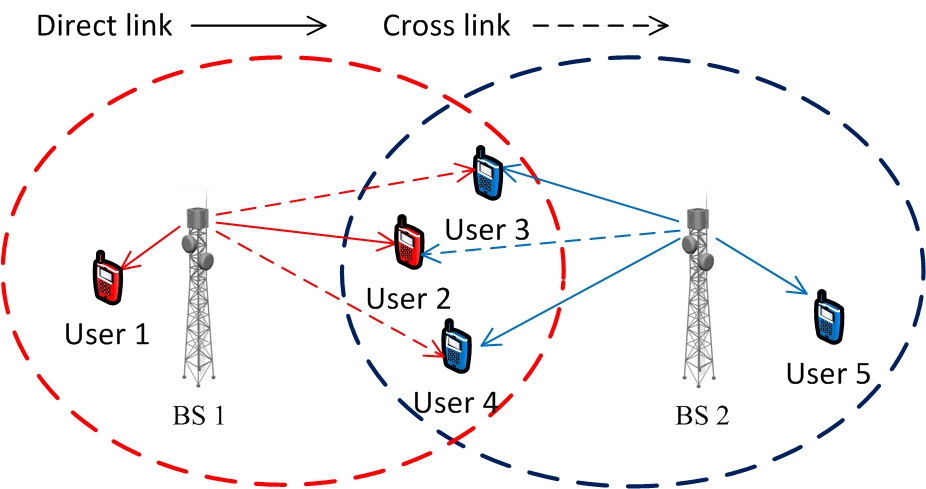
(a) A massive MIMO cellular network with $2$ BSs and $5$ users.

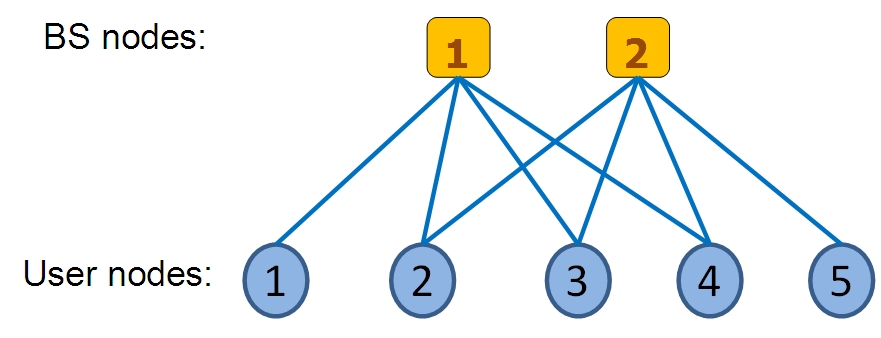
(b) The corresponding topology graph $\mathcal{G}_{T}\left(\mathbf{\Theta}\right)=\left\{\mathcal{B},\mathcal{U},\mathcal{E}\right\}$, where $\mathcal{B}=\left\{1,2\right\}$, $\mathcal{U}=\left\{1,2,3,4,5\right\}$ and $\mathcal{E}=\left\{\left(1,1\right),\left(1,2\right),\left(1,3\right),\left(1,4\right),\left(2,2\right),\left(2,3\right),\left(2,4\right),\left(2,5\right)\right\}$.

Figure 1: An example of massive MIMO cellular network and the corresponding topology graph.

Consider the downlink of a massive MIMO cellular network with $N$ BSs and $K$ single-antenna users as illustrated in Fig. 1 for $N=2$ and $K=5$. Each BS has $M$ antennas with $M$ much larger than the number of the associated users. Denote $\mathbf{h}_{k,n}\in\mathbb{C}^{M}$ as the channel vector between BS $n$ and user $k$. The channel fading process is modeled as $\mathbf{h}_{k,n}\left(t\right)=\sqrt{M}\mathbf{\Theta}_{k,n}^{1/2}\left(t\right)\mathbf{z}_{k,n}\left(t\right),\>\forall k,n$, where $\mathbf{z}_{k,n}\left(t\right)\in\mathbb{C}^{M}$ has i.i.d. complex entries of zero mean and variance $1/M$; and $\mathbf{\Theta}_{k,n}\left(t\right)\in\mathbb{C}^{M\times M}$ is the spatial correlation matrix between BS $n$ and user $k$. The random process $\mathbf{z}_{k,n}\left(t\right)$ is quasi-static within a time slot but i.i.d. w.r.t. time slots, user and BS indices $\left(t,k,n\right)$. The spatial correlation process $\mathbf{\Theta}_{k,n}\left(t\right)$ is assumed to be a slow ergodic process (i.e., $\mathbf{\Theta}_{k,n}\left(t\right)$ remains constant for a large number of time slots) according to a general distribution. As such, the CSI is divided into instantaneous CSI $\mathbf{H}=\left\{\mathbf{h}_{k,n}\right\}$ and global statistical information $\mathbf{\Theta}\triangleq\left\{\mathbf{\Theta}_{k,n}\right\}$ (spatial correlation matrices). Due to local scattering [7], the spatial correlation matrices of different users in cell $n$ is usually different. However, if the coverage area of a BS is partitioned into $N_{c}$ small sub-areas, it is reasonable to assume that any two users collocated in the same sub-area have almost the same spatial correlation matrices. This motivates us to consider the following locally-clustered spatial channel model.

Assumption 1 (Locally-clustered Spatial Channel).

The spatial correlation matrices $\left\{\mathbf{\Theta}_{k,n},\forall k\right\}$ associated with BS $n$ belongs to a finite set $\mathbf{\Psi}_{n}$ with the size $\left|\mathbf{\Psi}_{n}\right|=N_{c}$. Furthermore, due to the local spatial scattering [7], we have $\textrm{Rank}\left(\mathbf{\Theta}_{k,n}\right)<M,\>\forall k,n$. ∎

Assumption 1 is realistic because in practice, there are only limited number of significant eigenvalues in a MIMO channel (especially for large $M$). The massive MIMO cellular network can be represented by a topology graph as define below.

Definition 1 (Network Topology Graph).

For given spatial correlation matrices $\mathbf{\Theta}$, define the topology graph of the massive MIMO cellular network as a bipartite graph $\mathcal{G}_{T}\left(\mathbf{\Theta}\right)=\left\{\mathcal{B},\mathcal{U},\mathcal{E}\right\}$, where $\mathcal{B}$ denotes the set of all BS nodes, $\mathcal{U}$ denotes the set of all user nodes, and $\mathcal{E}$ is the set of all edges between the BSs and users. For each BS node $n$, let $\mathcal{U}_{n}$ denote the set of associated users and $\overline{\mathcal{U}}_{n}=\left\{k:\>k\notin\mathcal{U}_{n},\left(k,n\right)\in\mathcal{E}\right\}$ denote the set of neighbor users. For each user node $k$, let $b_{k}$ denote the index of its serving BS and $\mathcal{B}_{k}=\left\{n:\>n\neq b_{k},\left(k,n\right)\in\mathcal{E}\right\}$ denote the set of neighbor BSs. ∎

Define $\textrm{E}\left[\left\|\mathbf{h}_{k,n}\right\|^{2}\right]=\textrm{Tr}\left(\mathbf{\Theta}_{k,n}\right)$ as the path gain between BS $n$ and user $k$. An edge between a user node and a BS node in the network topology graph indicates there is strong path gain between these two nodes. This is stated formally below.

Definition 2 (Edge Set).

For given $\mathbf{\Theta}$, there is an edge $\left(k,n\right)\in\mathcal{E}$ between BS node $n\in\mathcal{B}$ and user node $k\in\mathcal{U}$ in the network topology graph $\mathcal{G}_{T}\left(\mathbf{\Theta}\right)=\left\{\mathcal{B},\mathcal{U},\mathcal{E}\right\}$ if $\textrm{Tr}\left(\mathbf{\Theta}_{k,b_{k}}\right)<\theta\textrm{Tr}\left(\mathbf{\Theta}_{k,n}\right)$, for some threshold $\theta>1$. ∎

Remark 1.

In practical wireless networks, the data rate of each user is limited by the available modulation and coding schemes (MCS) (e.g., the highest MCS in LTE is 64QAM, no coding [8]). If the path gain between a user and a BS is sufficiently small compared to the direct link path gain ($\theta$ times smaller than the direct link path gain), the interference from this BS will have negligible effect on the data rate of this user. Simulations show that the performance of the proposed scheme is not sensitive to the choice of $\theta$ for a wide range of $\theta$ from $5$dB to $20$dB.

An example of massive MIMO cellular network and the corresponding topology graph is illustrated in Fig. 1. For BS $1$, the set of associated users is $\mathcal{U}_{1}=\left\{1,2\right\}$, and the set of neighbor users is $\overline{\mathcal{U}}_{1}=\left\{3,4\right\}$. For user $2$, the index of the serving BS is $b_{2}=1$ and the set of neighbor BSs is $\mathcal{B}_{2}=\left\{2\right\}$. For user $3$, the index of the serving BS is $b_{3}=2$ and the set of neighbor BSs is $\mathcal{B}_{3}=\left\{1\right\}$.

At each time slot, linear precoding is employed at BS $n$ to support simultaneous downlink transmissions to a set of scheduled users denoted by $\mathcal{S}_{n}$. Let $\mathcal{S}=\cup_{n=1}^{N}\mathcal{S}_{n}$ denote the set of all the selected users and $\overline{\mathcal{S}}_{n}=\overline{\mathcal{U}}_{n}\cap\mathcal{S}$ denote the set of selected users who are neighbors of BS $n$. Note that a user $k\in\overline{\mathcal{S}}_{n}$ can be potentially interfered by BS $n$ because there is a cross link (edge) between BS $n$ and a user $k\in\overline{\mathcal{S}}_{n}$. For example, consider the massive MIMO cellular network in Fig. 1. Suppose the sets of selected users at the BSs are $\mathcal{S}_{1}=\left\{1,2\right\}$ and $\mathcal{S}_{2}=\left\{3,5\right\}$. Then, we have $\mathcal{S}=\mathcal{S}_{1}\cup\mathcal{S}_{2}=\left\{1,2,3,5\right\}$ and $\overline{\mathcal{S}}_{1}=\overline{\mathcal{U}}_{1}\cap\mathcal{S}=\left\{3\right\}$, where $\overline{\mathcal{U}}_{1}=\left\{3,4\right\}$. Since user $3$ has a cross link with BS $1$ as illustrated in Fig. 1-(a), it can be potentially interfered by BS $1$. Using the above notations, the received signal for a user $k$ can be expressed as:

$$y_{k} = \mathbf{h}_{k,b_{k}}^{\dagger}\sqrt{p_{k}}\mathbf{v}_{k}s_{k}+\underset{\textrm{intracell\>\ interference}}{\underbrace{\mathbf{h}_{k,b_{k}}^{\dagger}\sum_{l\in\mathcal{S}_{b_{k}}\backslash\{k\}}\sqrt{p_{l}}\mathbf{v}_{l}s_{l}}}$$

$$+\underset{\textrm{intercell\>\ interference}}{\underbrace{\sum_{n\in\mathcal{B}_{k}}\mathbf{h}_{k,n}^{\dagger}\mathbf{V}_{n}\mathbf{P}_{n}\mathbf{s}_{n}}}+n_{k},$$

where $s_{k}\sim\mathcal{CN}\left(0,1\right)$ is the data symbol, $p_{k}$ is the power allocation and $\mathbf{v}_{k}$ is the precoding vector of user $k$; $\mathcal{S}_{b_{k}}$ is the set of selected users at BS $b_{k}$; $\mathbf{s}_{n}=\left[s_{l}\right]_{l\in\mathcal{S}_{n}}\in\mathbb{C}^{\left|\mathcal{S}_{n}\right|}$ is the data symbol vector at BS $n$; $\mathbf{P}_{n}=\textrm{diag}\left(\mathbf{p}_{n}\right)$ and $\mathbf{p}_{n}=\left[p_{l}\right]_{l\in\mathcal{S}_{n}}\in\mathbb{R}_{+}^{\left|\mathcal{S}_{n}\right|}$ is the power allocation vector at BS $n$; $\mathbf{V}_{n}=\left[\mathbf{v}_{l}\right]_{l\in\mathcal{S}_{n}}\in\mathbb{C}^{M\times\left|\mathcal{S}_{n}\right|}$ is the precoding matrix at BS $n$; and $n_{k}\sim\mathcal{CN}\left(0,1\right)$ is the AWGN noise.

II-B Hierarchical Interference Mitigation

Conventional interference mitigation techniques for small scale MIMO cellular networks such as MU-MIMO precoding, coordinated MIMO [5], or cooperative MIMO [6], cannot be applied directly to massive MIMO cellular networks due to two practical challenges, namely, the insufficient pilot symbols for CSI estimation and the backhaul latency. To resolve these practical challenges, we propose a novel hierarchical interference mitigation control, which can fully utilize the large number of antennas to simultaneously mitigate the inter-cell interference as well as realize the spatial multiplexing gain per BS. Specifically, the interference mitigation strategy is partitioned into long-term and short-term controls. The short-term control is responsible to capture the spatial multiplexing gain among the intra-cell users at each BS based on the local CSIT only. On the other hand, the long-term control is responsible to mitigate the inter-cell interference based on the global statistical information. They are elaborated as follows.

II-B1 Hierarchical Precoding for Intra-cell and Inter-cell Interference Mitigation

We first use a simple example to illustrate the idea of hierarchical precoding.

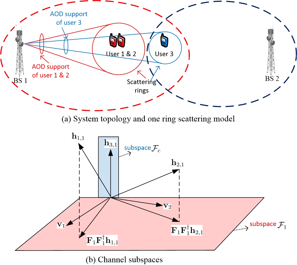
Figure 2: An example massive MIMO cellular network with one ring scattering model to illustrate the role of spatial correlation matrices $\mathbf{\Theta}$. The direct link channel subspace $\mathcal{F}$ is illustrated in Subfigure (b). It consists of two orthogonal subspaces $\mathcal{F}_{c}$ and $\mathcal{F}_{1}$.

Example 1.

Consider the massive MIMO cellular network in Fig. 2-(a). Each BS has $32$ antennas. Consider the one ring model in [9] for transmit antenna correlation, where a user is surrounded by a ring of scatterers such that the support of its Angle-of-Departure (AOD) distribution are restricted to a certain region as illustrated in Fig. 2-(a). Assume that user 1 and user 2 share the same scattering ring and $\mathbf{h}_{1,1},\mathbf{h}_{2,1}$ are restricted in the same 4-dimensional subspace $\mathcal{F}$ (i.e., $\textrm{span}\left(\mathbf{\Theta}_{1,1}\right)=\textrm{span}\left(\mathbf{\Theta}_{2,1}\right)=\mathcal{F}$) as illustrated in Fig. 2-(b). Moreover, due to the local scattering configuration as illustrated in Fig. 2-(a), the cross link channel vector $\mathbf{h}_{3,1}$ between BS 1 and user 3 is restricted in a 2-dimensional subspace $\mathcal{F}_{c}\subset\mathcal{F}$ (i.e., $\textrm{span}\left(\mathbf{\Theta}_{3,1}\right)=\mathcal{F}_{c}\subset\mathcal{F}$). We consider a hierarchical precoder structure for BS 1: $\mathbf{V}_{1}=\mathbf{F}_{1}\mathbf{G}_{1}$, where $\mathbf{F}_{1}\in\mathbb{U}^{32\times 2}$ with $\textrm{span}\left(\mathbf{F}_{1}\right)\subseteq\mathcal{F}$ is the outer precoder adaptive to the spatial correlation matrices $\mathbf{\Theta}$ only, and $\mathbf{G}_{1}\in\mathbb{C}^{2\times 2}$ is the inner precoder adaptive to the local CSI (the effective channel $\widetilde{\mathbf{H}}_{1}=\left[\mathbf{F}_{1}^{\dagger}\mathbf{h}_{1,1},\mathbf{F}_{1}^{\dagger}\mathbf{h}_{2,1}\right]^{\dagger}\in\mathbb{C}^{2\times 2}$).

We have the following observations from Example 1.

Role of spatial correlation matrices $\mathbf{\Theta}$: The knowledge of the spatial correlation matrices $\mathbf{\Theta}$ can be exploited to design the outer precoder $\mathbf{F}_{1}$ to eliminate the inter-cell interference to user $3$. Specifically, this can be achieved by setting $\mathbf{F}_{1}$ to be a set of orthogonal basis of a 2-dimensional subspace $\mathcal{F}_{1}$, where $\mathcal{F}_{1}\subset\mathcal{F}$ and $\mathcal{F}_{1}\perp\mathcal{F}_{c}$ as illustrated in Fig. 2-(b).

Role of local CSI $\widetilde{\mathbf{H}}_{1}$: The knowledge of local real-time instantaneous CSI $\widetilde{\mathbf{H}}_{1}$ can be exploited to design the inner precoder $\mathbf{G}_{1}$ to realize the spatial multiplexing gain at BS 1.

For general massive MIMO cellular networks, we propose a hierarchical precoder $\mathbf{V}_{n}=\mathbf{F}_{n}\mathbf{G}_{n}$ for each BS $n$ as illustrated in Fig. 3. The outer precoder $\mathbf{F}_{n}\in\mathbb{U}^{M\times M_{n}}$ with $M_{n}<M$ (we let $\mathbf{F}_{n}=\mathbf{0}$ if $M_{n}=0$) is used to eliminate the inter-cell interference and is adaptive to the global statistical information $\mathbf{\Theta}$. The inner precoder $\mathbf{G}_{n}\in\mathbb{C}^{M_{n}\times\left|\mathcal{S}_{n}\right|}$ is used to realize the spatial multiplexing gain at each BS and is adaptive to the local real-time CSI $\widetilde{\mathbf{H}}_{\mathcal{S}_{n}}\triangleq\left[\mathbf{F}_{n}^{\dagger}\mathbf{h}_{k,n}\right]_{k\in\mathcal{S}_{n}}^{\dagger}\in\mathbb{C}^{\left|\mathcal{S}_{n}\right|\times M_{n}}$. Define $\mathbf{F}=\left\{\mathbf{F}_{1},...,\mathbf{F}_{N}\right\}$ as the set of outer precoders for all BSs. By properly choosing $\mathbf{F}$ (equation (2)), one can eliminate the inter-cell interference as illustrated in Example 1.

Remark 2.

Physically, the rank $M_{n}$ of $\mathbf{F}_{n}$ means the number of data streams for spatial multiplexing at BS $n$. Due to limited spatial scattering [7], a BS with say $M=100$ antennas does not mean it can support spatial multiplexing of 100 data streams. In practice, there are just a few (say $10$) significant eigenchannels despite having 100 antennas, and having $M_{n}=10$ spatially multiplexed data streams already capture most of the spatial multiplexing advantage. The remaining spatial DoFs can be used for inter-cell interference mitigation.

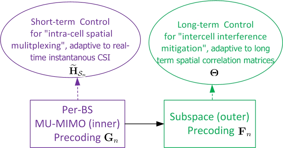
Figure 3: An illustration of hierarchical precoder structure.

For a given outer precoder $\mathbf{F}$, we consider regularized zero-forcing (RZF) inner precoder with a parameter $\nu$. The RZF precoder is easy to implement and is asymptotically optimal for $M,\left|\mathcal{S}_{n}\right|\rightarrow\infty$ [10]. Moreover, we can apply the technique of deterministic equivalent (DE) for RZF precoding in [11] to facilitate the algorithm design. For convenience, define the composite channel from BS $n$ to any subset of users $\mathcal{U}^{S}\subseteq\mathcal{U}$ as $\mathbf{H}_{\mathcal{U}^{S}}=\left[\mathbf{h}_{l,n}\right]_{l\in\mathcal{U}^{S}}^{\dagger}\in\mathbb{C}^{\left|\mathcal{U}^{S}\right|\times M}$. If the inter-cell interference is completely eliminated by the outer precoders $\mathbf{F}$, the RZF inner precoder is given by

$$\mathbf{G}_{n} = \left(\mathbf{F}_{n}^{\dagger}\mathbf{H}_{\mathcal{S}_{n}}^{\dagger}\mathbf{H}_{\mathcal{S}_{n}}\mathbf{F}_{n}+M\nu\mathbf{I}_{M_{n}}\right)^{-1}\mathbf{F}_{n}^{\dagger}\mathbf{H}_{\mathcal{S}_{n}}^{\dagger},$$ (1)

where $\nu>0$ is a fixed parameter for RZF. Note that $\nu$ is scaled by $M$ to ensure that the matrix $\mathbf{F}_{n}^{\dagger}\mathbf{H}_{\mathcal{S}_{n}}^{\dagger}\mathbf{H}_{\mathcal{S}_{n}}\mathbf{F}_{n}+M\nu\mathbf{I}_{M_{n}}$ is well conditioned as $M,\left|\mathcal{S}_{n}\right|\rightarrow\infty$.

II-B2 Statistical User Scheduling and Power Allocation

In [12], it has been observed that as the number of antennas $M$ grows large, the role of multi-user diversity gain (by selecting users based on instantaneous CSIT) becomes less and less effective because of “channel hardening”. Moreover, the benefits of short timescale power allocation (i.e., the power allocation is adaptive to instantaneous CSIT) becomes asymptotically negligible as $K,M\rightarrow\infty$ because the data rate of each user converges almost surely to a deterministic function of the power allocation vector $\mathbf{p}=\left[\mathbf{p}_{1}^{T},...,\mathbf{p}_{N}^{T}\right]^{T}$ as will be shown in Lemma 1. As such, the user selection set and power allocation is assumed to be adaptive to the global statistical information $\mathbf{\Theta}$ only. Specifically, the user selection and the outer precoder are chosen to satisfy the zero inter-cell interference constraint:

$$\mathbf{F}_{n}^{\dagger}\sum_{k\in\overline{\mathcal{S}}_{n}}\mathbf{\Theta}_{k,n}=\mathbf{0},\>\forall n,$$ (2)

and the power allocation has to satisfy a per-BS power constraint that will be elaborated later. Note that the inter-cell interference from BS $n$ to a user $k\in\overline{\mathcal{S}}_{n}$ can be expressed as $M\mathbf{z}_{k,n}^{\dagger}\mathbf{\Theta}_{k,n}\mathbf{F}_{n}\mathbf{G}_{n}\mathbf{P}_{n}\mathbf{G}_{n}^{\dagger}\mathbf{F}_{n}^{\dagger}\mathbf{\Theta}_{k,n}\mathbf{z}_{k,n}$. Since $\mathbf{\Theta}_{k,n}$ is positive semidefinite, setting $\mathbf{F}_{n}^{\dagger}\sum_{k\in\overline{\mathcal{S}}_{n}}\mathbf{\Theta}_{k,n}=\mathbf{0}$ is equivalent to setting $\mathbf{F}_{n}^{\dagger}\mathbf{\Theta}_{k,n}=\mathbf{0},\>\forall k\in\overline{\mathcal{S}}_{n}$. Hence, the constraint in (2) can be used to eliminate the inter-cell interference to all users in the system. In (2), we consider ZF criteria for inter-cell interference mitigation due to its simplicity and asymptotic optimality at high SNR. Similar ZF criteria has also been used in [9] to design pre-beamforming matrix based on spatial correlation matrices in single cell systems.

Remark 3 (Implementation Considerations).

In the proposed hierarchical interference mitigation, the long term controls such as outer precoding, statistical user selection and power allocation are implemented at a central node based on the global statistical information about the channel ($\mathbf{\Theta}$), while the short term control (inner precoding) is implemented locally at each BS based on the local real-time instantaneous CSI knowledge ($\widetilde{\mathbf{H}}_{\mathcal{S}_{n}}$). The proposed hierarchical precoding solution has several unique benefits regarding implementation. (a) Robust to CSI signaling latency in backhaul, (b) Resolve the issues of insufficient pilot and feedback overhead for real-time CSIT estimation in massive MIMO systems. For instance, the central node requires the global statistical information (spatial correlation matrices) $\mathbf{\Theta}$ to compute the long term controls $\left\{\mathbf{F},\mathcal{S},\mathbf{p}\right\}$. The spatial correlation matrices can be estimated via downlink training using some standard covariance matrix estimation technique [13] at the users and then fed back to the BSs. Since $\mathbf{\Theta}$ changes at a much slower time scale w.r.t. the time slot rate, such a design requires substantially less signaling overhead compared to the coordinated MIMO and is more robust w.r.t. to the backhaul latency. On the other hand, BS $n$ only needs to know the local real-time instantaneous CSI $\widetilde{\mathbf{H}}_{\mathcal{S}_{n}}\in\mathbb{C}^{\left|\mathcal{S}_{n}\right|\times M_{n}}$ for the inner precoder $\mathbf{G}_{n}$. This can be obtained via downlink channel estimation and channel feedback using conventional CSI signaling mechanisms in modern wireless systems such as LTE [14]. Since $M_{n}$ is substantially smaller than $M$, the issue of the huge downlink pilot and CSI feedback signaling overhead in massive MIMO is also alleviated by the hierarchical precoding design.

III Optimization Formulation for Hierarchical Interference Mitigation

We consider joint optimization of the outer precoders $\mathbf{F}$, the user selection $\mathcal{S}$, and the power allocation $\mathbf{p}=\left[\mathbf{p}_{1}^{T},...,\mathbf{p}_{N}^{T}\right]^{T}$; all of them are adaptive to the global statistical information $\mathbf{\Theta}$. Define $\Gamma=\left\{\mathbf{F},\mathcal{S},\mathbf{p}\right\}$ as a composite control variable. For given $\Gamma=\left\{\mathbf{F},\mathcal{S},\mathbf{p}\right\}$ that satisfies (2), the instantaneous data rate (treating interference as noise) of user $k$ is

$$r_{k}\left(\Gamma\right)=\textrm{log}\left(1+\frac{1\left(k\in\mathcal{S}\right)p_{k}\left|\mathbf{h}_{k,b_{k}}^{\dagger}\mathbf{v}_{k}\right|^{2}}{\sum_{l\in\mathcal{S}_{b_{k}}\backslash k}p_{l}\left|\mathbf{h}_{k,b_{k}}^{\dagger}\mathbf{v}_{l}\right|^{2}+1}\right),$$ (3)

where the precoders $\left[\mathbf{v}_{l}\right]_{l\in\mathcal{S}_{n}}=\mathbf{F}_{n}\mathbf{G}_{n},\forall n$ with the inner precoder $\mathbf{G}_{n}$ given by (1). The transmit power of BS $n$ is

$$P_{n}\left(\Gamma\right)=\;\;\;\;\;\;\;\;\;\;\;\;\;\;\;\;\;\;\;\;\;\;\;\;\;\;\;\;\;\;\;\;\;\;\;\;\;\;\;\;\;\;\;\;\;\;\;\;\;\;\;\;\;\;\;\;\;\;\;\;\;\;\;\;\;\;\;\;\;\;\;$$

$$\textrm{Tr}\left(\mathbf{P}_{n}\mathbf{H}_{\mathcal{S}_{n}}\mathbf{F}_{n}\left(\mathbf{F}_{n}^{\dagger}\mathbf{H}_{\mathcal{S}_{n}}^{\dagger}\mathbf{H}_{\mathcal{S}_{n}}\mathbf{F}_{n}+M\nu\mathbf{I}_{M_{n}}\right)^{-2}\mathbf{F}_{n}^{\dagger}\mathbf{H}_{\mathcal{S}_{n}}^{\dagger}\right).$$ (4)

Note that there may not always be enough spatial DoFs to eliminate the inter-cell interference to all the users. Hence, for a fixed composite control variable $\Gamma$, it is possible that only part of the users can be scheduled for transmission. For fairness considerations, we consider randomized control policy which realizes time-sharing between several composite control variables as defined below.

Definition 3 (Randomized Control Policy).

A randomized control policy $\Omega=\left\{\Xi,\mathbf{q}\right\}$ consists of a set of composite control variables $\Xi\triangleq\left\{\Gamma_{1},...,\Gamma_{\left|\Xi\right|}\right\}$ with $\left|\Xi\right|\leq K$ and a probability vector $\mathbf{q}\triangleq\left[q_{1},...,q_{\left|\Xi\right|}\right]^{T}$, where the $j$-th composite control variable in $\Xi$ is $\Gamma_{j}=\left\{\mathbf{F}\left(j\right),\mathcal{S}\left(j\right),\mathbf{p}\left(j\right)\right\}$; and $\mathbf{q}$ satisfies $q_{j}\in\left[0,1\right],\forall j;\>\sum_{j=1}^{\left|\Xi\right|}q_{j}=1$. At any time slot, the composite control variable $\Gamma_{j}$ is used with probability $q_{j}$, i.e., the outer precoders, the user selection set and the power allocation are respectively given by $\mathbf{F}\left(j\right)$, $\mathcal{S}\left(j\right)$ and $\mathbf{p}\left(j\right)$ with probability $q_{j}$. Moreover, define the set of feasible control policies under per-BS power constraint $P_{c}$ as

$$\Lambda\left(P_{c}\right)=\left\{\Omega\triangleq\left\{\Xi,\mathbf{q}\right\}:\>\Xi\subseteq\Xi^{\textrm{F}}\left(P_{c}\right)\right\},$$

where $\Xi^{\textrm{F}}\left(P_{c}\right)=\left\{\Gamma\in\Xi^{\textrm{A}}:\>\textrm{E}\left[\left.P_{n}\left(\Gamma\right)\right|\mathbf{\Theta}\right]\leq P_{c}\right\}$ is the set of feasible composite control variables, and $\Xi^{\textrm{A}}=\left\{\Gamma:\>\mathbf{F}_{n}^{\dagger}\sum_{k\in\overline{\mathcal{S}}_{n}}\mathbf{\Theta}_{k,n}=\mathbf{0},\forall n\right.$ $\left.\>\textrm{and}\>\underset{k\in\mathcal{S}}{\textrm{sup}}p_{k}<\infty\right\}$ is the set of admissible composite control variables. ∎

For given control policy $\Omega=\left\{\Xi,\mathbf{q}\right\}$ and spatial correlation matrices $\mathbf{\Theta}$, the conditional average data rate of user $k$ is:

$$\overline{r}_{k}\left(\Omega|\mathbf{\Theta}\right)=\sum_{j=1}^{\left|\Xi\right|}q_{j}\textrm{E}\left[\left.r_{k}\left(\Gamma_{j}\right)\right|\mathbf{\Theta}\right].$$

The network performance is characterized by a utility function $U\left(\overline{\mathbf{r}}\left(\Omega|\mathbf{\Theta}\right)\right)$, where $\overline{\mathbf{r}}\left(\Omega|\mathbf{\Theta}\right)=\left[\overline{r}_{1}\left(\Omega|\mathbf{\Theta}\right),...,\overline{r}_{K}\left(\Omega|\mathbf{\Theta}\right)\right]^{T}$ is the conditional average rate vector. We make the following assumptions on $U\left(\overline{\mathbf{r}}\right)$ ($\overline{\mathbf{r}}$ is a simplified notation for $\overline{\mathbf{r}}\left(\Omega|\mathbf{\Theta}\right)$).

Assumption 2 (Assumptions on Utility).

The utility function can be expressed as $U\left(\overline{\mathbf{r}}\right)\triangleq\sum_{k=1}^{K}w_{k}u\left(\overline{r}_{k}\right)$, where $w_{k}\geq 0$ is the weight for user $k$, $u\left(r\right)$ is assumed to be a twice differentiable, concave and increasing function for all $r\geq 0$. Moreover, $u\left(r\right)$ is L-Lipschitz, i.e.,

$$\left|\frac{\partial u\left(r_{1}\right)}{\partial r}-\frac{\partial u\left(r_{2}\right)}{\partial r}\right|\leq L\left|r_{1}-r_{2}\right|,\forall r_{1},r_{2}\geq 0,$$

for some constant $L>0$.

The above utility function captures a lot of interesting cases:

• Alpha-fair [15]: Alpha-fair can be used to compromise between the fairness to users and the utilization of resources. The utility function is

  $$U\left(\overline{\mathbf{r}}\right)=\begin{cases}\frac{1}{K}\sum_{k=1}^{K}\textrm{log}\left(\overline{r}_{k}+\epsilon\right),&\alpha=1,\\ \frac{1}{K}\sum_{k=1}^{K}\left(1-\alpha\right)^{-1}\left(\overline{r}_{k}+\epsilon\right)^{1-\alpha},&\textrm{otherwise},\end{cases}$$ (5)

  where $\epsilon>0$ is a small number.

• Proportional Fair (PFS) [16]: This is a special case of alpha-fair when $\alpha=1$.

For a given topology graph $\mathcal{G}_{T}\left(\mathbf{\Theta}\right)=\left\{\mathcal{B},\mathcal{U},\mathcal{E}\right\}$ and per-BS power constraint $P_{c}$, the problem of interference mitigation via hierarchical precoding can be formulated as:

$$\mathcal{P}\left(\mathcal{G}_{T}\left(\mathbf{\Theta}\right)\right):\>\underset{\Omega}{\textrm{max}}\>U\left(\overline{\mathbf{r}}\left(\Omega|\mathbf{\Theta}\right)\right),\>\textrm{s.t.}\>\Omega\in\Lambda\left(P_{c}\right).$$

Note that the conditional average rate $\overline{r}_{k}\left(\Omega|\mathbf{\Theta}\right)$ in the utility function and the conditional average power $\textrm{E}\left[\left.P_{n}\left(\Gamma\right)\right|\mathbf{\Theta}\right]$ in the constraint function of $\mathcal{P}\left(\mathcal{G}_{T}\left(\mathbf{\Theta}\right)\right)$ do not have closed form expressions. To make the problem tractable, we need to address the following challenge.

Challenge 1 (Closed Form Approximation for $\mathcal{P}\left(\mathcal{G}_{T}\left(\mathbf{\Theta}\right)\right)$).

Find an approximated problem $\mathcal{P}_{E}\left(\mathcal{G}_{T}\left(\mathbf{\Theta}\right)\right)$ with closed form objective and constraints such that the solution of $\mathcal{P}_{E}\left(\mathcal{G}_{T}\left(\mathbf{\Theta}\right)\right)$ is asymptotically optimal w.r.t. $\mathcal{P}\left(\mathcal{G}_{T}\left(\mathbf{\Theta}\right)\right)$ as $M$ grows large.

We resort to random matrix theory to solve the above challenge. Specifically, we first derive deterministic equivalents (DEs) [11] for the conditional average rate and power. Then we obtain an approximated problem $\mathcal{P}_{E}\left(\mathcal{G}_{T}\left(\mathbf{\Theta}\right)\right)$ by replacing the conditional average rate and power with their DE approximations. Finally, we show that the solution of $\mathcal{P}_{E}\left(\mathcal{G}_{T}\left(\mathbf{\Theta}\right)\right)$ is an $O\left(\nu\right)$-optimal solution of $\mathcal{P}\left(\mathcal{G}_{T}\left(\mathbf{\Theta}\right)\right)$.

Definition 4 ($O\left(\nu\right)$-optimal solution).

A solution $\Omega=\left\{\Xi,\mathbf{q}\right\}$ is called an $O\left(\nu\right)$-feasible solution of $\mathcal{P}\left(\mathcal{G}_{T}\left(\mathbf{\Theta}\right)\right)$ if it satisfies the zero inter-cell interference constraint $\mathbf{F}_{n}^{\dagger}\left(j\right)\sum_{k\in\overline{\mathcal{S}}_{n}\left(j\right)\triangleq\overline{\mathcal{U}}_{n}\cap\mathcal{S}\left(j\right)}\mathbf{\Theta}_{k,n}=\mathbf{0},\forall n,j$ and the following relaxed per-BS power constraint

$$\textrm{E}\left[\left.P_{n}\left(\Gamma_{j}\right)\right|\mathbf{\Theta}\right]-P_{c}\leq O\left(\nu\right),\>\forall j.$$

It is called an $O\left(\nu\right)$-optimal solution of $\mathcal{P}\left(\mathcal{G}_{T}\left(\mathbf{\Theta}\right)\right)$ if it is an $O\left(\nu\right)$-feasible solution and $U^{*}-U\left(\overline{\mathbf{r}}\left(\Omega|\mathbf{\Theta}\right)\right)\leq O\left(\nu\right)$, where $U^{*}$ is the optimal objective value of $\mathcal{P}\left(\mathcal{G}_{T}\left(\mathbf{\Theta}\right)\right)$.

Throughout the paper, the notation $M\rightarrow\infty$ refers to $M\rightarrow\infty$ and $\left|\mathcal{U}_{n}\right|\rightarrow\infty,\forall n$ such that $0<\underset{M\rightarrow\infty}{\liminf}\left|\mathcal{U}_{n}\right|/M\leq\underset{M\rightarrow\infty}{\limsup}\left|\mathcal{U}_{n}\right|/M<\infty$. For technical reasons, we require the following assumptions.

Assumption 3 (Technical Assumptions for DE).

 

1. All spatial correlation matrices $\mathbf{\Theta}_{k,n},\forall k,n$ have uniformly bounded spectral norm on $M$, i.e.,

   $$\underset{M\rightarrow\infty}{\limsup}\underset{1\leq k\leq K}{\textrm{sup}}\left\|\mathbf{\Theta}_{k,n}\right\| < \infty,\>\forall n.$$ (6)

   Moreover, $\underset{M\rightarrow\infty}{\liminf}\frac{1}{M}\textrm{Rank}\left(\sum_{k\in\mathcal{U}_{n}}\mathbf{\Theta}_{k,n}\right)>0$.

2. All the random matrices $\frac{1}{M}\mathbf{H}_{\mathcal{U}_{n}}\mathbf{H}_{\mathcal{U}_{n}}^{\dagger},\forall n$ have uniformly bounded spectral norm on $M$ with probability one, i.e.,

   $$\underset{M\rightarrow\infty}{\limsup}\left\|\frac{1}{M}\mathbf{H}_{\mathcal{U}_{n}}\mathbf{H}_{\mathcal{U}_{n}}^{\dagger}\right\| \overset{a.s}{<} \infty,\>\forall n.$$

3. $w_{k}=O\left(1/K\right),\>k=1,...,K$. ∎

Assumption 3-1) is satisfied by many MIMO channel models such as the angular domain MIMO channel model in [7] and it is a standard assumption in the literatures, see e.g., [11, 17]. Under Assumption 3-1), Assumption 3-2) holds true if $\underset{M\rightarrow\infty}{\limsup}\left|\left\{\mathbf{\Theta}_{k,n}:\>k\in\mathcal{U}_{n}\right\}\right|<\infty$, that is, if $\left\{\mathbf{\Theta}_{k,n}:\>k\in\mathcal{U}_{n}\right\}$ belongs to a finite family [11]. According to the locally-clustered channel model in Assumption 1, we have$\left|\left\{\mathbf{\Theta}_{k,n}:\>k\in\mathcal{U}_{n}\right\}\right|\leq N_{c}$ and thus Assumption 3-2) holds true. Assumption 3-3) is to ensure that the utility function is bounded as $K\rightarrow\infty$.

Lemma 1 (DE of Rate and Power).

Let Assumption 3 hold true and consider composite control variable $\Gamma=\left\{\mathbf{F},\mathcal{S},\mathbf{p}\right\}$ satisfying: 1) $\Gamma\in\Xi^{\textrm{A}}$; 2) the corresponding user selection $\mathcal{S}_{n}$ satisfies $0<\underset{M\rightarrow\infty}{\liminf}\left|\mathcal{S}_{n}\right|/M\leq\underset{M\rightarrow\infty}{\limsup}\left|\mathcal{S}_{n}\right|/M<\infty$. Then for any BS $n$, we have

$$\lim_{M\rightarrow\infty}\left|r_{k}\left(\Gamma\right)-r_{k}^{\circ}\left(\Gamma|\mathbf{\Theta}\right)\right| \overset{a.s}{\leq} O\left(\nu\right),\>\forall k\in\mathcal{S}_{n},$$

$$\lim_{M\rightarrow\infty}\left|P_{n}\left(\Gamma\right)-P_{n}^{\circ}\left(\Gamma|\mathbf{\Theta}\right)\right| \overset{a.s}{\leq} O\left(\nu\right),$$

for sufficiently small $\nu>0$, where

$$r_{k}^{\circ}\left(\Gamma|\mathbf{\Theta}\right) = \log\left(1+p_{k}\right),\>\forall k\in\mathcal{S}_{n},$$ (7)

$$P_{n}^{\circ}\left(\Gamma|\mathbf{\Theta}\right) = \frac{1}{M}\sum_{i\in\mathcal{S}_{n}}\frac{p_{i}}{\xi_{i}},$$ (8)

are the deterministic equivalent (DE) of user rate and BS transmit power, and $\xi_{i},\forall i\in\mathcal{S}_{n}$ form the unique solution of

$$\xi_{i} = \frac{1}{M}\textrm{Tr}\left(\tilde{\mathbf{\Theta}}_{i,n}\mathbf{T}_{n}\right),$$

$$\mathbf{T}_{n} = \left(\frac{1}{M}\sum_{j\in\mathcal{S}_{n}}\frac{\tilde{\mathbf{\Theta}}_{j,n}}{\nu+\xi_{j}}+\mathbf{I}_{M}\right)^{-1},$$ (9)

with $\tilde{\mathbf{\Theta}}_{i,n}=\mathbf{F}_{n}\mathbf{F}_{n}^{\dagger}\mathbf{\Theta}_{i,n}\mathbf{F}_{n}\mathbf{F}_{n}^{\dagger},\forall i\in\mathcal{S}_{n}$.

Please refer to Appendix -A for the proof.

Remark 4.

Note that the above DEs are established on the "conditional distribution of the channel" (conditioned on the statistics $\mathbf{\Theta}$). Given a realization of $\mathbf{\Theta}$ (the statistics), the control actions $\Gamma=\left\{\mathbf{F},\mathcal{S},\mathbf{p}\right\}$ are all fixed (because they are adaptive to $\mathbf{\Theta}$ only). As such, the conditional measure of $\mathbf{H}$ (conditioned on the given $\mathbf{\Theta}$) will exhibit “random matrix theory” behavior and the DE convergence in Lemma 1 can be proved using standard techniques in [11]. On the other hand, if $\mathcal{S}$ were adaptive to the instantaneous CSI $\mathbf{H}$ (short-term user selection), then conditioned on $\mathbf{\Theta}$, $\mathcal{S}$ would be random and hence the DE approximation would fail (due to the random $\mathcal{S}$ or extreme value effect of the user selection which changes the underlying conditional distribution of the channels $\mathbf{H}$). Similar conclusion has also been made in [9] that the DE of the data rate in massive MIMO system is valid as long as the user selection is independent of the instantaneous CSI $\mathbf{H}$.

Based on Lemma 1, we have the following result.

Theorem 1 (Asymptotic $O\left(\nu\right)$-equivalence of $\mathcal{P}\left(\mathcal{G}_{T}\left(\mathbf{\Theta}\right)\right)$).

Let $\Omega^{\star}$ denote the optimal solution of

$$\mathcal{P}_{E}\left(\mathcal{G}_{T}\left(\mathbf{\Theta}\right)\right):\>\underset{\Omega}{\textrm{max}}\>U_{E}\left(\Omega\right)\triangleq\sum_{k=1}^{K}w_{k}u\left(\sum_{j=1}^{\left|\Xi\right|}q_{j}r_{k}^{\circ}\left(\Gamma_{j}|\mathbf{\Theta}\right)\right)$$

$$\textrm{s.t.}\>\Omega\in\Lambda^{\circ}\left(P_{c}\right).\;\;\;\;\;\;\;\;\;\;\;\;\;\;\;\;\;\;\;\;\;\;\;\;\;\;\;\;\;\;\;\;\;\;\;\;\;\;\;\;\;$$

where $\Lambda^{\circ}\left(P_{c}\right)=\left\{\Omega\triangleq\left\{\Xi,\mathbf{q}\right\}:\>\Xi\subseteq\Xi^{\textrm{F}\circ}\left(P_{c}\right)\right\}$, and $\Xi^{\textrm{F}\circ}\left(P_{c}\right)=\left\{\Gamma\in\Xi^{\textrm{A}}:\>P_{n}^{\circ}\left(\Gamma|\mathbf{\Theta}\right)\leq P_{c}\right\}$. Given Assumption 3 and for sufficiently small $\nu>0$, $\Omega^{\star}$ is an $O\left(\nu\right)$-optimal solution of $\mathcal{P}\left(\mathcal{G}_{T}\left(\mathbf{\Theta}\right)\right)$ as $M\rightarrow\infty$. ∎

Please refer to Appendix -B for the proof. By Theorem 1, the solution of $\mathcal{P}\left(\mathcal{G}_{T}\left(\mathbf{\Theta}\right)\right)$ can be approximated by the solution of $\mathcal{P}_{E}$, and the approximation is $O\left(\nu\right)$-optimal as $M\rightarrow\infty$.

IV Solution of $\mathcal{P}_{E}\left(\mathcal{G}_{T}\left(\mathbf{\Theta}\right)\right)$

In the rest of the paper, we focus on solving $\mathcal{P}_{E}\left(\mathcal{G}_{T}\left(\mathbf{\Theta}\right)\right)$ for fixed $\mathbf{\Theta}$. We will use $\mathcal{G}_{T}$, $r_{k}^{\circ}\left(\Gamma\right)$ and $P_{n}^{\circ}\left(\Gamma\right)$ as simplified notations for $\mathcal{G}_{T}\left(\mathbf{\Theta}\right)$, $r_{k}^{\circ}\left(\Gamma|\mathbf{\Theta}\right)$ and $P_{n}^{\circ}\left(\Gamma|\mathbf{\Theta}\right)$ when there is no ambiguity. Clearly, the utility function $U_{E}\left(\Omega\right)$ is not a convex function on $\Omega$ and thus $\mathcal{P}_{E}\left(\mathcal{G}_{T}\right)$ is a non-convex optimization problem. Moreover, the optimization variables in $\mathcal{P}_{E}\left(\mathcal{G}_{T}\right)$ involve a set of composite control variables $\Xi$ with undetermined size and the associated probabilities $\mathbf{q}$ with undetermined dimension. It is in general very difficult to find the global optimal solution for such a non-convex problem. In this section, we are going to address the following challenge.

Challenge 2 (Design a Global Convergent Algorithm for $\mathcal{P}_{E}\left(\mathcal{G}_{T}\right)$).

Exploit the specific structure of problem $\mathcal{P}_{E}\left(\mathcal{G}_{T}\right)$ to design an iterative algorithm that converges to the global optimal solution of $\mathcal{P}_{E}\left(\mathcal{G}_{T}\right)$.

We first study the optimality condition of $\mathcal{P}_{E}\left(\mathcal{G}_{T}\right)$. Then we propose an iterative algorithm to solve Challenge 2.

IV-A Global Optimality Condition of $\mathcal{P}_{E}\left(\mathcal{G}_{T}\right)$

It is difficult to find a simple characterization for the necessary and sufficient global optimality condition of a general non-convex problem. However, problem $\mathcal{P}_{E}\left(\mathcal{G}_{T}\right)$ is not an arbitrary non-convex problem but has some specific hidden convexity structure, which can be exploited to derive the global optimality condition for $\mathcal{P}_{E}\left(\mathcal{G}_{T}\right)$ as shown below.

We first study the hidden convexity of $\mathcal{P}_{E}\left(\mathcal{G}_{T}\right)$. Define the (deterministic equivalent of) average rate region as:

$$\mathcal{R}\triangleq\underset{\Omega\in\Lambda^{\circ}\left(P_{c}\right)}{\bigcup}\left\{\mathbf{x}\in\mathbb{R}_{+}^{K}:\>\mathbf{x}\leq\overline{\mathbf{r}}^{\circ}\left(\Omega\right)\right\},$$ (10)

where $\overline{\mathbf{r}}^{\circ}\left(\Omega\right)=\left[\overline{r}_{1}^{\circ}\left(\Omega\right),...,\overline{r}_{K}^{\circ}\left(\Omega\right)\right]^{T}$ with $\overline{r}_{k}^{\circ}\left(\Omega\right)=\sum_{j=1}^{\left|\Xi\right|}q_{j}r_{k}^{\circ}\left(\Gamma_{j}\right)$. Then we have the following Lemma.

Lemma 2 (Convexity of $\mathcal{R}$).

$\mathcal{R}=\textrm{Conv}\left(\mathcal{R}^{\textrm{F}}\right)$, where $\textrm{Conv}\left(\cdot\right)$ denotes the convex hull operation and $\mathcal{R}^{\textrm{F}}\triangleq\left\{\mathbf{r}^{\circ}\left(\Gamma\right)=\left[r_{1}^{\circ}\left(\Gamma\right),...,r_{K}^{\circ}\left(\Gamma\right)\right]^{T}:\Gamma\in\Xi^{\textrm{F}\circ}\left(P_{c}\right)\right\}$.

Please refer to Appendix -C for the proof.

The following lemma shows that problem $\mathcal{P}_{E}\left(\mathcal{G}_{T}\right)$ is equivalent to a convex problem:

$$\underset{\overline{\mathbf{r}}^{\circ}}{\textrm{max}}U\left(\overline{\mathbf{r}}^{\circ}\right)\triangleq\sum_{k=1}^{K}w_{k}u\left(\overline{r}_{k}^{\circ}\right),\>\textrm{s.t.}\>\overline{\mathbf{r}}^{\circ}=\left[\overline{r}_{1}^{\circ},...,\overline{r}_{K}^{\circ}\right]^{T}\in\mathcal{R},$$ (11)

Lemma 3 (Equivalence between $\mathcal{P}_{E}\left(\mathcal{G}_{T}\right)$ and (11)).

If $\Omega^{\star}$ is the global optimal solution of $\mathcal{P}_{E}\left(\mathcal{G}_{T}\right)$, then $\overline{\mathbf{r}}^{\circ}\left(\Omega^{\star}\right)$ is the optimal solution of problem (11); on the other hand, if $\overline{\mathbf{r}}^{\circ\star}$ is the optimal solution of problem (11), then any $\Omega^{\star}$ satisfying $\overline{\mathbf{r}}^{\circ}\left(\Omega^{\star}\right)=\overline{\mathbf{r}}^{\circ\star}$ is also the global optimal solution of $\mathcal{P}_{E}\left(\mathcal{G}_{T}\right)$.

Please refer to Appendix -C for the proof. This hidden convexity of $\mathcal{P}_{E}\left(\mathcal{G}_{T}\right)$ (i.e., the equivalence between $\mathcal{P}_{E}\left(\mathcal{G}_{T}\right)$ and (11)) is the key to derive the global optimality condition of $\mathcal{P}_{E}\left(\mathcal{G}_{T}\right)$. Note that although problem (11) is convex, the solution is still non-trivial because there is no simple characterization for its feasible set $\mathcal{R}$.

To derive the global optimality condition of $\mathcal{P}_{E}\left(\mathcal{G}_{T}\right)$, we also need the first order optimality condition of problem (11) as summarized in the following lemma.

Lemma 4 (First Order Optimality Condition of (11)).

A solution $\overline{\mathbf{r}}^{\circ\star}=\left[\overline{r}_{1}^{\circ\star},...,\overline{r}_{K}^{\circ\star}\right]^{T}$ is optimal for problem (11) if and only if

$$\nabla^{T}U\left(\overline{\mathbf{r}}^{\circ\star}\right)\left(\overline{\mathbf{r}}^{\circ\star}-\mathbf{x}\right)\geq 0,\forall\mathbf{x}\in\mathcal{R}.$$ (12)

Finally, from Lemma 3 and Lemma 4, we can obtain the necessary and sufficient global optimality condition for problem $\mathcal{P}_{E}\left(\mathcal{G}_{T}\right)$ as follows.

Theorem 2 (Global Optimality Condition of $\mathcal{P}_{E}\left(\mathcal{G}_{T}\right)$).

A control policy $\Omega^{\star}=\left\{\Xi^{\star},\mathbf{q}^{\star}\right\}$ with $\Xi^{\star}=\left\{\Gamma_{1}^{\star},...,\Gamma_{\left|\Xi^{\star}\right|}^{\star}\right\}$ is a global optimal solution of $\mathcal{P}_{E}\left(\mathcal{G}_{T}\right)$ if and only if $\Gamma_{j}^{\star},\forall j\in\left\{1,...,\left|\Xi^{\star}\right|\right\}$ satisfies:

$$\boldsymbol{\mu}^{\star T}\left(\mathbf{r}^{\circ}\left(\Gamma_{j}^{\star}\right)-\mathbf{r}^{\circ}\left(\Gamma\right)\right)\geq 0,\>\forall\Gamma\in\Xi^{\textrm{F}\circ}\left(P_{c}\right),$$ (13)

where $\mathbf{r}^{\circ}\left(\Gamma\right)=\left[r_{1}^{\circ}\left(\Gamma\right),...,r_{K}^{\circ}\left(\Gamma\right)\right]^{T}$ and the weight vector $\boldsymbol{\mu}^{\star}\triangleq\nabla U\left(\overline{\mathbf{r}}^{\circ}\left(\Omega^{\star}\right)\right)=\left[w_{k}\frac{\partial u\left(r\right)}{\partial r}|_{r=\overline{r}_{k}^{\circ}\left(\Omega^{\star}\right)}\right]_{k=1,...,K}$.

The detailed proof can be found in Appendix -C.

IV-B Global Optimal Solution of $\mathcal{P}_{E}\left(\mathcal{G}_{T}\right)$

Just as we can obtain the optimal solution of a convex problem by solving its KKT conditions, we can also obtain the global optimal solution of $\mathcal{P}_{E}\left(\mathcal{G}_{T}\right)$ by solving the global optimality condition in Theorem 2. Specifically, for any given spatial correlation matrices $\mathbf{\Theta}$, we propose Algorithm E to achieve the global optimality condition of $\mathcal{P}_{E}\left(\mathcal{G}_{T}\left(\mathbf{\Theta}\right)\right)$ by iteratively updates the optimization variables $\Xi,\mathbf{q}$ and the weight vector $\boldsymbol{\mu}$ in Theorem 2.

Algorithm E (Top level algorithm for solving $\mathcal{P}_{E}\left(\mathcal{G}_{T}\left(\mathbf{\Theta}\right)\right)$):

Initialization: Set $i=0$ and let $\boldsymbol{\mu}^{(0)}=\left[w_{k}\right]_{k=1,...,K}$. Call Procedure $\textrm{W}^{\star}$ with input $\boldsymbol{\mu}^{(0)}$ to obtain a composite control variable $\Gamma^{\star}\left(\boldsymbol{\mu}^{(0)}\right)$ and let $\Xi^{(0)}=\left\{\Gamma^{\star}\left(\boldsymbol{\mu}^{(0)}\right)\right\}$.

Step 1 (Update probability vector $\mathbf{q}$): Call Procedure Q with input $\Xi^{(i)}=\left\{\Gamma_{1}^{(i)},...,\Gamma_{\left|\Xi^{(i)}\right|}^{(i)}\right\}$ to obtain the updated probability vector $\mathbf{q}^{(i)}=\left[q_{j}^{(i)}\right]_{j=1,...,\left|\Xi^{(i)}\right|}$. Let $\widetilde{\Xi}^{(i)}=\left\{\Gamma_{j}^{(i)}:\>j\in\mathcal{J}^{(i)}\right\}$ and $\widetilde{\mathbf{q}}^{(i)}=\left[q_{j}^{(i)}\right]_{j\in\mathcal{J}^{(i)}}$, where $\mathcal{J}^{(i)}=\left\{j:\>q_{j}^{(i)}>0\right\}$. Let $\Omega^{(i)}=\left\{\widetilde{\Xi}^{(i)},\widetilde{\mathbf{q}}^{(i)}\right\}$

Step 2 (Update composite control variable set $\Xi$): Let

$$\boldsymbol{\mu}^{(i+1)}=\nabla U\left(\overline{\mathbf{r}}^{\circ}\left(\Omega^{(i)}\right)\right)\triangleq\left[w_{k}\frac{\partial u\left(r\right)}{\partial r}|_{r=\overline{r}_{k}^{\circ}\left(\Omega^{(i)}\right)}\right]_{k=1,...,K}.$$ (14)

Call Procedure $\textrm{W}^{\star}$ with input $\boldsymbol{\mu}^{(i+1)}$ to obtain a new composite control variable $\Gamma^{\star}\left(\boldsymbol{\mu}^{(i+1)}\right)$. Update $\Xi$ as

$$\Xi^{(i+1)}=\widetilde{\Xi}^{(i)}\cup\Gamma^{\star}\left(\boldsymbol{\mu}^{(i+1)}\right).$$ (15)

Step 3: If $i>0$ and $\left|U_{E}\left(\Omega^{(i)}\right)-U_{E}\left(\Omega^{(i-1)}\right)\right|\leq\varepsilon$, where $\varepsilon>0$ is a small number, terminate the algorithm. Otherwise, let $i=i+1$ and return to Step 1.

Figure 4: Summary of overall solution and the inter-relationship of the algorithm components for both Algorithm E (with Procedure $\textrm{W}^{\star}$, composite control variable $\Gamma^{\star}\left(\boldsymbol{\mu}\right)$ and output $\Omega^{\star}=\left\{\Xi^{\star},\mathbf{q}^{\star}\right\}$) and the modified Algorithm E (with Procedure W, composite control variable $\hat{\Gamma}\left(\boldsymbol{\mu}\right)$ and output $\hat{\Omega}=\left\{\hat{\Xi},\hat{\mathbf{q}}\right\}$). The iteration number ⁽ⁱ⁾ is omitted for simplicity. Each square represents an algorithm component and the corresponding square bracket explains the function of this algorithm component.

Fig. 4 summarizes the inter-relationship between the components of Algorithm E. Algorithm E contains two procedures (subroutines) which will be elaborated below.

Remark 5.

Algorithm E can be interpreted as the Frank-Wolfe Algorithm (also known as the conditional gradient algorithm) with exact line search [18] applied on the equivalent convex problem in (11). Compared to the conventional Frank-Wolfe Algorithm, the main difference is that the optimization variable in problem $\mathcal{P}_{E}\left(\mathcal{G}_{T}\right)$ is $\Omega$ instead of $\overline{\mathbf{r}}^{\circ}$ in (11), and the optimization w.r.t. $\Omega$ is non-convex. Nonetheless, we can exploit the hidden convexity (global optimality condition) in Theorem 2 to establish the global convergence of Algorithm E as will be shown in Theorem 4.

IV-B1 Procedure Q (Optimization of $\mathbf{q}$ for fixed $\Xi$)

For given input $\Xi$, Procedure Q essentially solves the optimal probability vector $\mathbf{q}$ for $\mathcal{P}_{E}\left(\mathcal{G}_{T}\right)$ with fixed $\Xi$, i.e., Procedure Q with input $\Xi$ is a standard convex optimization procedure to solve the following optimization problem:

$$\underset{\left[q_{j}\right]_{j=1,...,\left|\Xi\right|}}{\max}\sum_{k=1}^{K}w_{k}u\left(\sum_{j=1}^{\left|\Xi\right|}q_{j}r_{k}^{\circ}\left(\Gamma_{j}\right)\right),$$ (16)

$$\textrm{s.t.}\>q_{j}\in\left[0,1\right],\forall j\>\textrm{and}\>\sum_{j=1}^{\left|\Xi\right|}q_{j}=1,$$

where $\Gamma_{j}$ is the $j$-th composite control variable in $\Xi$. Hence, Procedure Q can be efficiently implemented by existing convex optimization methods/software. As such, the pseudo code of Procedure Q is omitted here for conciseness.

IV-B2 Procedure $\textrm{W}^{\star}$ (Finding a new composite control variable for given $\boldsymbol{\mu}$)

The pseudo code of Procedure $\textrm{W}^{\star}$ is summarized in Table I. In Line 2, $\xi_{i},\forall i\in\mathcal{S}_{n}$ is the unique solution of (9) with $\tilde{\mathbf{\Theta}}_{i,n}=\tilde{\mathbf{\Theta}}_{i,n}\left(\overline{\mathcal{S}}_{n}\right)\triangleq\left(\mathbf{I}_{M}-\mathbf{U}\left(\overline{\mathcal{S}}_{n}\right)\mathbf{U}^{\dagger}\left(\overline{\mathcal{S}}_{n}\right)\right)\mathbf{\Theta}_{i,n}\left(\mathbf{I}_{M}-\mathbf{U}\left(\overline{\mathcal{S}}_{n}\right)\mathbf{U}^{\dagger}\left(\overline{\mathcal{S}}_{n}\right)\right)$, where $\mathbf{U}\left(\overline{\mathcal{S}}_{n}\right)=\textrm{orth}\left(\sum_{k\in\overline{\mathcal{S}}_{n}}\mathbf{\Theta}_{k,n}\right)$. In Line 4, $R\left(\mathcal{S}\right)$ is the (deterministic equivalent of) weighted sum-rate for given user selection $\mathcal{S}$. In Line 7, $\overline{\mathcal{S}}_{n}^{\star}=\overline{\mathcal{U}}_{n}\cap\mathcal{S}^{\star}$. For convenience, $\xi_{k}$ is referred to as the effective channel gain of user $k$ and $\tilde{\mathbf{\Theta}}_{i,n}\left(\overline{\mathcal{S}}_{n}\right)$ is called the projected spatial correlation matrix of user $i$. For conciseness, $\tilde{\mathbf{\Theta}}_{i,n}\left(\overline{\mathcal{S}}_{n}\right)$ is denoted as $\tilde{\mathbf{\Theta}}_{i,n}$ when there is no ambiguity. To calculate the weighted sum-rate $R\left(\mathcal{S}\right)$, we need to obtain the effective channel gains $\xi_{i},\forall i\in\mathcal{S}$ associated with $\mathcal{S}$ by solving the fixed point equation in (9). The solution of (9) can be obtained using the following fixed point iterations [11]

$$\xi_{i}^{(t+1)}=\frac{1}{M}\textrm{Tr}\left(\tilde{\mathbf{\Theta}}_{i,n}\left(\frac{1}{M}\sum_{j\in\mathcal{S}_{n}}\frac{\tilde{\mathbf{\Theta}}_{j,n}}{\nu+\xi_{j}^{(t)}}+\mathbf{I}_{M}\right)^{-1}\right),$$ (17)

with initial point $\xi_{i}^{(0)}=1,\forall i\in\mathcal{S}_{n}$, where $\tilde{\mathbf{\Theta}}_{i,n}=\tilde{\mathbf{\Theta}}_{i,n}\left(\overline{\mathcal{S}}_{n}\right),\forall i\in\mathcal{S}_{n}$.

Table I: Procedure $\textrm{W}^{\star}$ (for solving Condition (18))

1. For all $\mathcal{S}$

2.    Let $p_{k}^{\star}\left(\mathcal{S}\right)=\left(\frac{\mu_{k}M\xi_{k}}{\lambda_{b_{k}}}-1\right)^{+},\forall k$, where $\lambda_{b_{k}}$ is

3.    chosen such that $\frac{1}{M}\sum_{i\in\mathcal{S}_{b_{k}}}\frac{p_{i}^{\star}\left(\mathcal{S}\right)}{\xi_{i}}=P_{c}$.

4.    Let $R\left(\mathcal{S}\right)=\sum_{k\in\mathcal{S}}\mu_{k}\textrm{log}\left(1+p_{k}^{\star}\left(\mathcal{S}\right)\right)$.

5. End

6. Let $\mathcal{S}^{\star}=\underset{\mathcal{S}}{\textrm{argmax}}R\left(\mathcal{S}\right)$ and $\mathbf{p}^{\star}=\left[p_{k}^{\star}\left(\mathcal{S}^{\star}\right)\right]_{k\in\mathcal{S}^{\star}}$.

7. Let $\mathbf{F}_{n}^{\star}=\textrm{orth}\left(\left(\mathbf{I}_{M}-\mathbf{U}\left(\overline{\mathcal{S}}_{n}^{\star}\right)\mathbf{U}^{\dagger}\left(\overline{\mathcal{S}}_{n}^{\star}\right)\right)\sum_{k\in\mathcal{S}_{n}^{\star}}\mathbf{\Theta}_{k,n}\right)$.

8. Output $\Gamma^{\star}\left(\boldsymbol{\mu}\right)=\left\{\mathbf{F}^{\star},\mathcal{S}^{\star},\mathbf{p}^{\star}\right\}$, where $\mathbf{F}^{\star}=\left\{\mathbf{F}_{1}^{\star},...,\mathbf{F}_{N}^{\star}\right\}$.

For given input $\boldsymbol{\mu}$, Procedure $\textrm{W}^{\star}$ essentially finds a composite control variable $\Gamma^{\star}\left(\boldsymbol{\mu}\right)$ which satisfies the global optimality condition in (13) for fixed $\boldsymbol{\mu}$.

Theorem 3 (Characterization of Procedure $\textrm{W}^{\star}$).

For given input $\boldsymbol{\mu}$, the output $\Gamma^{\star}\left(\boldsymbol{\mu}\right)$ of Procedure $\textrm{W}^{\star}$ satisfies

$$\boldsymbol{\mu}^{T}\left(\mathbf{r}^{\circ}\left(\Gamma^{\star}\left(\boldsymbol{\mu}\right)\right)-\mathbf{r}_{k}^{\circ}\left(\Gamma\right)\right)\geq 0,\>\forall\Gamma\in\Xi^{\textrm{F}\circ}\left(P_{c}\right).$$ (18)

Please refer to Appendix -D for the proof.

IV-B3 Convergence and Performance of Algorithm E

The update rule in Algorithm E is designed according to the global optimality condition in Theorem 2. As a result, it can be shown that Algorithm E converges to the global optimal solution of $\mathcal{P}_{E}\left(\mathcal{G}_{T}\right)$ using the global optimality condition in Theorem 2 and the property of Algorithm E in the following Lemma.

Lemma 5 (Property of Algorithm E).

Let $\Omega^{(i)}$ be the control policy in the $i$-th iteration of Algorithm E. We have

$$U_{E}\left(\Omega^{(i+1)}\right)\geq$$

$$\max_{\eta\in\left[0,1\right]}U\left(\left(1-\eta\right)\overline{\mathbf{r}}^{\circ}\left(\Omega^{(i)}\right)+\eta\mathbf{r}^{\circ}\left(\Gamma^{\star}\left(\boldsymbol{\mu}^{(i+1)}\right)\right)\right),$$ (19)

where $\boldsymbol{\mu}^{(i+1)}=\nabla U\left(\overline{\mathbf{r}}^{\circ}\left(\Omega^{(i)}\right)\right)$ is given in (14).

Please refer to Appendix -E for the proof.

Using Theorem 2 and Lemma 5, we obtain the following global convergence result.

Theorem 4 (Global Optimality of Algorithm E).

Algorithm E monotonically increases the utility $U_{E}\left(\Omega^{(i)}\right)$ and $\lim_{i\rightarrow\infty}U_{E}\left(\Omega^{(i)}\right)\rightarrow U^{\star}$, where $U^{\star}$ is the global optimal value of $\mathcal{P}_{E}\left(\mathcal{G}_{T}\right)$.

Please refer to Appendix -E for the proof.

In step 2 of Algorithm E, we need to call Procedure $\textrm{W}^{\star}$, which involves an exhaustive user selection process where $R\left(\mathcal{S}\right)$ is calculated for all possible user set $\mathcal{S}$ (see Line 1 to Line 6 of Procedure $\textrm{W}^{\star}$). The complexity of exhaustive user selection is exponential w.r.t. the number of users $K$. In the next subsection, we will propose a low complexity solution, named the modified Algorithm E, for $\mathcal{P}_{E}\left(\mathcal{G}_{T}\right)$ by replacing the exhaustive user selection process with a statistical greedy user selection process.

IV-C Low Complexity Solution of $\mathcal{P}_{E}\left(\mathcal{G}_{T}\right)$

The low complexity solution (modified Algorithm E) is obtained by replacing the exact solution $\Gamma^{\star}\left(\boldsymbol{\mu}\right)$ of (18) in step 2 (and the initialization step) of Algorithm E with an approximate solution $\hat{\Gamma}\left(\boldsymbol{\mu}\right)$ found by a low complexity procedure named Procedure W. In other words, the modified Algorithm E are the same as Algorithm E except that Procedure $\textrm{W}^{\star}$ (which involves exhaustive user selection) is replaced by the low complexity counterpart Procedure W (which is based on statistical greedy user selection).

The pseudo code of Procedure W is summarized in Table II. In Line 3 and 4, the weighted sum-rate $R\left(\mathcal{S}\right)$ for any given $\mathcal{S}$ can be calculated using the same method as described in Procedure $\textrm{W}^{\star}$. Clearly, the statistical greedy user selection loop between Line 2 and Line 9 converges to a solution $\hat{\mathcal{S}}$ within $K$ iterations.

Table II: Procedure W (for solving Condition (18))

1. Initialization: Let $\mathcal{S}=\emptyset$ and $\textrm{Add\_flag}=1$.

2.  while $\textrm{Add\_flag}==1$ and $\left|\mathcal{S}\right|<K$

3.    Let $\mathcal{S}^{\circ}=\textrm{argmax}{}_{\mathcal{S}^{{}^{\prime}}\in\left\{\mathcal{S}\cup\left\{k\right\}:\>\forall k\in\mathcal{U}\backslash\mathcal{S}\right\}}\>R\left(\mathcal{S}^{{}^{\prime}}\right)$.

4.    if $R\left(\mathcal{S}^{\circ}\right)>R\left(\mathcal{S}\right)$ then

5.      $\mathcal{S}=\mathcal{S}^{\circ}$.

6.    else

7.      $\textrm{Add\_flag}=0$.

8.    end if

9.  end while

10. Let $\hat{\mathcal{S}}=\mathcal{S}$ and $\hat{\mathbf{p}}=\left[p_{k}^{\star}\left(\mathcal{S}\right)\right]_{k\in\mathcal{S}}$.

11. Let $\hat{\mathbf{F}}_{n}=\textrm{orth}\left(\left(\mathbf{I}_{M}-\mathbf{U}\left(\overline{\mathcal{S}}_{n}\right)\mathbf{U}^{\dagger}\left(\overline{\mathcal{S}}_{n}\right)\right)\sum_{k\in\mathcal{S}_{n}}\mathbf{\Theta}_{k,n}\right)$.

12. Output $\hat{\Gamma}\left(\boldsymbol{\mu}\right)=\left\{\hat{\mathbf{F}},\hat{\mathcal{S}},\hat{\mathbf{p}}\right\}$, where $\hat{\mathbf{F}}=\left\{\hat{\mathbf{F}}_{1},...,\hat{\mathbf{F}}_{N}\right\}$.

Fig. 4 summarizes the overall low complexity solution and the inter-relationship between the components of the modified Algorithm E. To justify the modified Algorithm E, we need to address the following challenge.

Challenge 3 (Monotone Convergence of the modified Algorithm E).

Prove the monotone convergence of the modified Algorithm E as well as characterize the performance loss of the modified Algorithm E w.r.t. the global optimal solution.

The following theorem provides a solution to Challenge 3.

Theorem 5 (Convergence of the Modified Alg. E).

The modified Algorithm E monotonically increases the utility $U_{E}\left(\Omega^{(i)}\right)$ and $\lim_{i\rightarrow\infty}U_{E}\left(\Omega^{(i)}\right)\rightarrow\hat{U}$. Moreover, the gap of $\hat{U}$ with the optimal utility $U_{E}^{\star}$ of $\mathcal{P}_{E}\left(\mathcal{G}_{T}\right)$ is bounded by

$$U_{E}^{\star}-\hat{U}\leq\hat{\boldsymbol{\mu}}^{T}\left(\mathbf{r}_{k}^{\circ}\left(\Gamma^{\star}\left(\hat{\boldsymbol{\mu}}\right)\right)-\mathbf{r}_{k}^{\circ}\left(\hat{\Gamma}\left(\hat{\boldsymbol{\mu}}\right)\right)\right),$$

where $\left(\hat{\overline{\mathbf{r}}}_{k}^{\circ},\hat{\boldsymbol{\mu}}\right)$ can be any accumulation point of the iterates $\left\{\overline{\mathbf{r}}^{\circ}\left(\Omega^{(i)}\right),\boldsymbol{\mu}^{(i+1)}\right\}$ generated by the modified Algorithm E, $\Gamma^{\star}\left(\hat{\boldsymbol{\mu}}\right)$ is the output of Procedure $\textrm{W}^{\star}$ with input $\hat{\boldsymbol{\mu}}$ and $\hat{\Gamma}\left(\hat{\boldsymbol{\mu}}\right)$ is the output of Procedure W with input $\hat{\boldsymbol{\mu}}$.

Please refer to Appendix -F for the proof. Theorem 5 states that the performance gap between the modified Algorithm E and (the optimal) Algorithm E is upper bounded by the performance gap (in terms of weighted sum-rate) between Procedure W (statistical user selection) and Procedure $\textrm{W}^{\star}$ (exhaustive user selection).

Complexity Analysis for the Modified Algorithm E

The computation complexity is evaluated in terms of the number of matrix multiplications, matrix inversions and Gram–Schmidt processes, since these operations dominate the first order of the overall computation complexity. For simplicity, we assume $\textrm{Rank}\left(\mathbf{\Theta}_{i,n}\right)=d,\forall i,n$ and $\left|\overline{\mathcal{U}}_{n}\right|=\overline{K},\forall n$. Suppose that the fixed point iterations in (17) converges to the desired accuracy in $C_{f}$ iterations. Then the complexity of Procedure W is analyzed as follows. In each iteration, the greedy search to find the $\mathcal{S}^{\circ}$ requires evaluating $K-\left|\mathcal{S}\right|<K$ weighted sum-rates $R\left(\mathcal{S}^{{}^{\prime}}\right)$. Each $R\left(\mathcal{S}^{{}^{\prime}}\right)$ needs no more than $O\left(C_{f}\left|\mathcal{S}\right|\right)$ $M\times M$ matrix multiplications and $O\left(NC_{f}\right)$ $M\times M$ matrix inversions. The greedy search is repeated for at most $K$ times. For each $n$, $\tilde{\mathbf{\Theta}}_{i,n},\forall i\in\mathcal{U}_{n}$ is updated for at most $K\overline{K}$ times, and each update needs one $M\times M$ Gram–Schmidt processes (i.e., Gram–Schmidt processes for a $M\times M$ matrix) to calculate $\textrm{orth}\left(\sum_{j\in\overline{\mathcal{S}}_{n}^{{}^{\prime}}}\mathbf{\Theta}_{j,n}\right)$. Hence, the overall complexity of Procedure W is upper bounded by $O\left(K^{3}C_{f}\right)$ $M\times M$ matrix multiplications, $O\left(K^{2}NC_{f}\right)$ $M\times M$ matrix inversions and $O\left(NK\overline{K}\right)$ $M\times M$ Gram–Schmidt processes. This is also the order of the per iteration complexity for the modified Algorithm E because in each iteration of the modified Algorithm E, the computation complexity is dominated by Procedure W.

V Simulation Results

Figure 5: Topology of a cellular network with $19$ cells.

Consider a cellular network with $19$ cells as illustrated in Fig. 5. The inter-site distance is $500$m. In each cell, there are $2$ uniformly distributed hotspots with a radius of $50$m. There are $12$ users in one cell, $2/3$ of whom are clustered around the hotspots, while the others are uniformly distributed within the cell. Each BS is equipped with $M=48$ antennas. The spatial correlation matrices are generated according to $\mathbf{\Theta}_{k,n}=L_{k,n}\check{\mathbf{\Theta}}_{k,n},\forall k,n$, where the path gains $L_{k,n}$’s are generated using the path loss model (“Urban Macro NLOS” model) in [19], and the normalized spatial correlation matrices $\check{\mathbf{\Theta}}_{k,n}$’s with $\textrm{Tr}\left(\check{\mathbf{\Theta}}_{k,n}\right)=M$ and $\textrm{Rank}\left(\mathbf{\Theta}_{k,n}\right)=6$ are randomly generated. In the simulations, we set the threshold in Definition 2 as $\theta=10$dB and the parameter for RZF as $\nu=10^{-2}$. We compare the performance of the proposed algorithm with the following two baselines.

Baseline 1 (FFR): Fractional frequency reuse (FFR) [20] is applied to suppress the inter-cell interference. In each cell, ZF beamforming is used to serve the users on each subband.

Baseline 2 (Clustered CoMP): 3 neighbor BSs form a cluster and employ cooperative ZF [21] to simultaneously serve all the users within the cluster.

V-A Convergence of the Modified Algorithm E

Consider the PFS utility $U\left(\overline{\mathbf{r}}\right)=\frac{1}{K}\sum_{k=1}^{K}\textrm{log}\left(\overline{r}_{k}+\epsilon\right)$ with $\epsilon=10^{-4}$. The per BS transmit power is $P_{c}=10$dB. In Fig. 6, we plot the objective value $U_{E}\left(\Omega\right)$ of $\mathcal{P}_{E}$ versus the number of iterations of the modified Algorithm E. It can be seen that the modified Algorithm $E$ quickly converges.

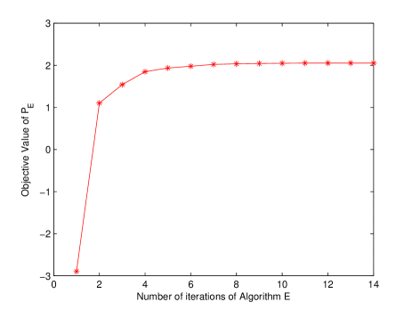
Figure 6: Objective value of $\mathcal{P}_{E}$ versus the number of iterations.

V-B Performance Evaluation under PFS Utility

The simulation setup is the same as that in Fig. 6. In Fig. 7, we compare the average cell throughput of different schemes under different backhaul latencies. For baseline 2, the $3$ cooperative BSs need to exchange CSI and payload data, and thus there is CSI delay when the backhaul latency is not zero. When there is CSI delay, the outdated CSI is related to the actual CSI by the autoregressive model in [22]. It can be seen that the cell throughput of the proposed scheme is close to the baseline 2 with zero backhaul latency and is much larger than baseline 1. The worst 10% users also benefit from huge throughput gain over baseline 1. Although the performance of baseline 2 is promising at zero backhaul latency, the performance quickly degrades at 10ms backhaul latency. These results demonstrated the superior performance and the robustness of the proposed hierarchical interference mitigation w.r.t. signaling latency in backhaul. Table III compares the computational complexity (CPU time) and signaling overhead of different schemes. The computational complexity and the backhaul signaling overhead of the proposed scheme are similar to FFR, and are much lower than CoMP. The real-time CSI estimation overhead of the proposed scheme is lower than both FFR and CoMP.

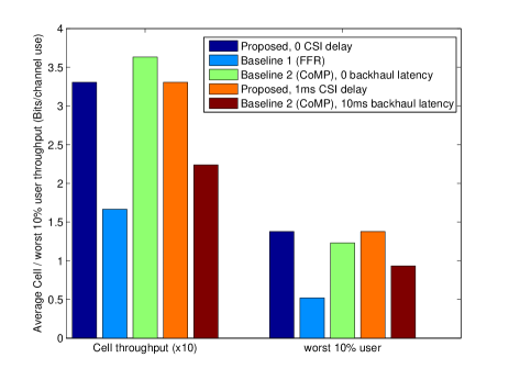
Figure 7: Throughput comparisons over different schemes. The user speed is 3 km/h.

	CPU	Backhaul	Real-time CSI
	time	signaling	estimation overhead
		overhead	(Pilot & CSI feedback)
Proposed	0.0260 s	34.23Mbps	$\approx$22 PS, 9 $\mathbb{C}^{22}$
FFR	0.0126 s	16.95Mbps	48 PS, 12 $\mathbb{C}^{48}$
CoMP	0.1006 s	111.2Mbps	48 PS, 12 $\mathbb{C}^{144}$

Table III: Comparison of the per time slot MATLAB computational time and per time slot per cell signaling overhead of different schemes. Assume that the system bandwidth is 1MHz, and the spatial channel correlation matrices $\mathbf{\Theta}$ changes every 1000 time slots. The other simulation setup is the same as Fig. 7. The real-time CSI estimation overhead includes the pilot symbol overhead (in terms of the average number of independent pilot symbols) and the uplink CSI feedback overhead (in terms of the average number of feedback channel vectors with different dimensions). For example, the real-time CSI estimation overhead of the proposed scheme is about “22 PS, 9 $\mathbb{C}^{22}$”, which means that in average, the proposed scheme requires transmitting 22 independent pilot symbols and feedbacking 9 complex channel vectors with average dimension $22$ per time slot per cell.

V-C Performance Evaluation under Sum-rate Utility

Consider the sum-rate utility. In Fig. 8, we plot the average cell throughput $\frac{K}{N}U\left(\overline{\mathbf{r}}\right)$ of different schemes versus the per BS transmit power $P_{c}$. It can be seen that the cell throughput of the proposed scheme is close to the baseline 2 with zero backhaul latency and is much larger than baseline 1. When there is a backhaul latency of 10ms, the proposed scheme also has a significant throughput gain over baseline 2. The DE of the cell throughput $\frac{K}{N}U_{E}\left(\Omega\right)$ is also plotted for the proposed scheme. It can be seen that the DE is very accurate.

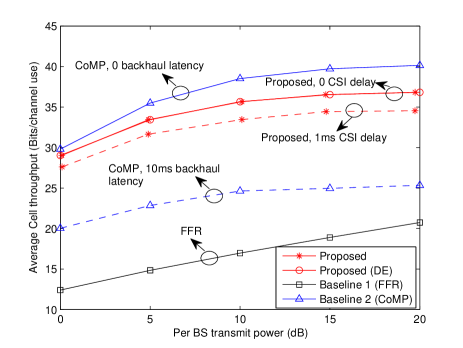
Figure 8: Average cell throughput versus the per BS transmit power $P_{c}$. The user speed is 3 km/h.

VI Conclusion

We propose a hierarchical interference mitigation scheme for massive MIMO cellular networks. The MIMO precoder is partitioned into inner precoder (for intra-cell interference control) and outer precoder (for inter-cell interference control). We study joint optimization of the outer precoders, the user selection, and the power allocation. The optimization only requires the knowledge of spatial correlation matrices and thus is robust to backhaul latency. We first apply the random matrix theory to obtain an approximated problem which is non-convex. Then using the hidden convexity of the problem, we propose Algorithm E to obtain the global optimal solution and a low complexity version of Algorithm E to find a sub-optimal solution. Simulations show that the proposed design achieves significant performance gain over various state-of-the-art baselines.

-A Proof of Lemma 1

Under the zero inter-cell interference constraint in (2), the $n$-th cell can be viewed as a single-cell downlink system with equivalent channels $\mathbf{F}_{n}\mathbf{F}_{n}^{\dagger}\mathbf{h}_{k,n},\forall k\in\mathcal{S}_{n}$. Throughout this proof, the notation $M\rightarrow\infty$ refers to $M\rightarrow\infty$ such that $0<\underset{M\rightarrow\infty}{\liminf}\left|\mathcal{S}_{n}\right|/M\leq\underset{M\rightarrow\infty}{\limsup}\left|\mathcal{S}_{n}\right|/M<\infty$. Following similar analysis as in the proof of [11, Theorem 2], the following lemma can be proved.

Lemma 6.

Let Assumption 3 holds true. As $M\rightarrow\infty$, we have $r_{k}\left(\Gamma\right)-\hat{r}_{k}^{\circ}\left(\Gamma\right)\overset{a.s}{\rightarrow}0$ and $P_{n}\left(\Gamma\right)-\hat{P}_{n}^{\circ}\left(\Gamma\right)\overset{a.s}{\rightarrow}0$, where

$$\hat{r}_{k}^{\circ}\left(\Gamma\right) = \textrm{log}\left(1+\frac{p_{k}\xi_{k}^{2}}{\nu^{2}\Upsilon_{k}+\left(\nu+\xi_{k}\right)^{2}}\right),$$ (20)

$$\hat{P}_{n}^{\circ}\left(\Gamma\right) = \frac{1}{M}\sum_{i\in\mathcal{S}_{n}}\frac{p_{i}\nu^{2}e_{i}}{\left(\nu+\xi_{i}\right)^{2}},$$ (21)

where $\Upsilon_{k}=\frac{1}{M}\sum_{i\in\mathcal{S}_{n}\backslash\left\{k\right\}}\frac{\nu^{2}p_{i}e_{ik}}{\left(\nu+\xi_{i}\right)^{2}}$; $\mathbf{e}=\left[e_{i}\right]_{i\in\mathcal{S}_{n}}\in\mathbb{R}^{\left|\mathcal{S}_{n}\right|}$ and $\mathbf{e}_{k}=\left[e_{ki}\right]_{i\in\mathcal{S}_{n}}\in\mathbb{R}^{\left|\mathcal{S}_{n}\right|}$ are given by

$$\mathbf{e} = \left(\mathbf{I}-\mathbf{J}\right)^{-1}\mathbf{u},$$ (22)

$$\mathbf{e}_{k} = \left(\mathbf{I}-\mathbf{J}\right)^{-1}\mathbf{u}_{k},$$ (23)

with $\mathbf{J}=\left[J_{ij}\right]_{i\in\mathcal{S}_{n},j\in\mathcal{S}_{n}}\in\mathbb{R}^{\left|\mathcal{S}_{n}\right|\times\left|\mathcal{S}_{n}\right|}$, $\mathbf{u}=\left[u_{i}\right]_{i\in\mathcal{S}_{n}}\in\mathbb{R}^{\left|\mathcal{S}_{n}\right|}$, and $\mathbf{u}_{k}=\left[u_{ki}\right]_{i\in\mathcal{S}_{n}}\in\mathbb{R}^{\left|\mathcal{S}_{n}\right|}$ given by

$$J_{ij}=\frac{\frac{1}{M}\textrm{tr}\tilde{\mathbf{\Theta}}_{i,n}\mathbf{T}_{n}\tilde{\mathbf{\Theta}}_{j,n}\mathbf{T}_{n}}{M\left(\nu+\xi_{j}\right)^{2}},$$

$$u_{ki}=\frac{1}{\nu^{2}M}\textrm{tr}\tilde{\mathbf{\Theta}}_{i,n}\mathbf{T}_{n}\tilde{\mathbf{\Theta}}_{k,n}\mathbf{T}_{n}, u_{i}=\frac{1}{\nu^{2}M}\textrm{tr}\tilde{\mathbf{\Theta}}_{i,n}\mathbf{T}_{n}^{2}.$$

Following similar analysis as in the proof of [11, Theorem 3], it can be shown that $\Upsilon_{k}=O\left(1\right)$ and $\nu^{2}e_{i}=\xi_{i}+O\left(\nu\right)$. Then it follows that $\frac{p_{k}\xi_{k}^{2}}{\nu^{2}\Upsilon_{k}+\left(\nu+\xi_{k}\right)^{2}}=p_{k}+O\left(\nu\right)$ and $\hat{P}_{n}^{\circ}\left(\Gamma\right)=\frac{1}{M}\sum_{i\in\mathcal{S}_{n}}\frac{p_{i}}{\xi_{i}}+O\left(\nu\right)$. From this and Lemma 6, Lemma 1 follows immediately.

-B Proof of Theorem 1

Let $\Omega^{*}$ be the optimal solution of Problem $\mathcal{P}\left(\mathcal{G}_{T}\right)$. It can be proved by contradiction that the control policies $\Omega^{*}$ and $\Omega^{\star}$ must satisfy: $\forall j$, $0<\underset{M\rightarrow\infty}{\liminf}\left|\mathcal{S}^{*}\left(j\right)\right|/M\leq\underset{M\rightarrow\infty}{\limsup}\left|\mathcal{S}^{*}\left(j\right)\right|/M<\infty$ and $0<\underset{M\rightarrow\infty}{\liminf}\left|\mathcal{S}^{\star}\left(j\right)\right|/M\leq\underset{M\rightarrow\infty}{\limsup}\left|\mathcal{S}^{\star}\left(j\right)\right|/M<\infty$. Define two sets

$$\mathcal{B}_{\infty}^{*}\left(j\right) = \left\{n:\>0<\underset{M\rightarrow\infty}{\liminf}\frac{\left|\mathcal{S}_{n}^{*}\left(j\right)\right|}{M}\leq\underset{M\rightarrow\infty}{\limsup}\frac{\left|\mathcal{S}_{n}^{*}\left(j\right)\right|}{M}<\infty\right\},$$

$$\mathcal{B}_{\infty}^{\star}\left(j\right) = \left\{n:\>0<\underset{M\rightarrow\infty}{\liminf}\frac{\left|\mathcal{S}_{n}^{\star}\left(j\right)\right|}{M}\leq\underset{M\rightarrow\infty}{\limsup}\frac{\left|\mathcal{S}_{n}^{\star}\left(j\right)\right|}{M}<\infty\right\}.$$

Let $\hat{\Omega}^{*}=\left\{\hat{\Xi}^{*},\mathbf{\hat{q}}^{*}\right\}$ denote a control policy that satisfies $\left|\hat{\Xi}^{*}\right|=\left|\Xi^{*}\right|$, $\hat{\mathbf{F}}_{n}^{*}\left(j\right)=\mathbf{F}_{n}\left(j\right),\hat{\mathcal{S}}_{n}^{*}\left(j\right)=\mathcal{S}_{n}^{*}\left(j\right),\hat{\mathbf{p}}_{n}^{*}\left(j\right)=\mathbf{p}_{n}^{*}\left(j\right),\forall n\in\mathcal{B}_{\infty}^{*}\left(j\right)$, and $\hat{\mathcal{S}}_{n}^{*}\left(j\right)=\emptyset,\forall n\notin\mathcal{B}_{\infty}^{*}\left(j\right)$. Let $\hat{\Omega}^{\star}=\left\{\hat{\Xi}^{\star},\mathbf{\hat{q}}^{\star}\right\}$ denote a control policy that satisfies $\left|\hat{\Xi}^{\star}\right|=\left|\Xi^{\star}\right|$, $\hat{\mathbf{F}}_{n}^{\star}\left(j\right)=\mathbf{F}_{n}\left(j\right),\hat{\mathcal{S}}_{n}^{\star}\left(j\right)=\mathcal{S}_{n}^{\star}\left(j\right),\hat{\mathbf{p}}_{n}^{\star}\left(j\right)=\mathbf{p}_{n}^{\star}\left(j\right),\forall n\in\mathcal{B}_{\infty}^{\star}\left(j\right)$, and $\hat{\mathcal{S}}_{n}^{\star}\left(j\right)=\emptyset,\forall n\notin\mathcal{B}_{\infty}^{\star}\left(j\right)$. It can be shown that as $M\rightarrow\infty$, we have

$$U\left(\overline{\mathbf{r}}\left(\hat{\Omega}|\mathbf{\Theta}\right)\right)\rightarrow U\left(\overline{\mathbf{r}}\left(\Omega|\mathbf{\Theta}\right)\right),\>U_{E}\left(\hat{\Omega}\right)\rightarrow U_{E}\left(\Omega\right).$$ (24)

for $\Omega=\Omega^{*},\hat{\Omega}=\hat{\Omega}^{*}$ or $\Omega=\Omega^{\star},\hat{\Omega}=\hat{\Omega}^{\star}$.

For composite control variable $\Gamma$ satisfying the conditions in Lemma 1, it can be shown that $r_{k}\left(\Gamma\right)$ and $P_{n}\left(\Gamma\right)$ are uniformly integrable [23] w.r.t. $M$. Together with Lemma 1, it follows that

$$\underset{M\rightarrow\infty}{\textrm{lim }}\left|\textrm{E}\left[\left.r_{k}\left(\Gamma\right)\right|\mathbf{\Theta}\right]-r_{k}^{\circ}\left(\Gamma|\mathbf{\Theta}\right)\right| \leq O\left(\nu\right),$$ (25)

$$\underset{M\rightarrow\infty}{\textrm{lim }}\left|\textrm{E}\left[\left.P_{n}\left(\Gamma\right)\right|\mathbf{\Theta}\right]-P_{n}^{\circ}\left(\Gamma|\mathbf{\Theta}\right)\right| \leq O\left(\nu\right),$$ (26)

By definition, we have

$$P_{n}^{\circ}\left(\hat{\Gamma}_{j}^{\star}|\mathbf{\Theta}\right)-P_{c} \leq 0,\forall j$$ (27)

Then it follows from (26) and (27) that

$$\textrm{E}\left[\left.P_{n}\left(\hat{\Gamma}_{j}^{\star}\right)\right|\mathbf{\Theta}\right]-P_{c}\leq O\left(\nu\right),\>\textrm{as}\>M\rightarrow\infty.$$ (28)

Similarly, it can be shown that

$$P_{n}^{\circ}\left(\hat{\Gamma}_{j}^{*}|\mathbf{\Theta}\right)-P_{c}\leq O\left(\nu\right),\>\textrm{as}\>M\rightarrow\infty.$$ (29)

We expand $U\left(\overline{\mathbf{r}}\left(\hat{\Omega}^{*}|\mathbf{\Theta}\right)\right)-U\left(\overline{\mathbf{r}}\left(\hat{\Omega}^{\star}|\mathbf{\Theta}\right)\right)$ as follows

$$U\left(\overline{\mathbf{r}}\left(\hat{\Omega}^{*}|\mathbf{\Theta}\right)\right)-U\left(\overline{\mathbf{r}}\left(\hat{\Omega}^{\star}|\mathbf{\Theta}\right)\right)=\left[U_{E}\left(\hat{\Omega}^{*}\right)-U_{E}\left(\hat{\Omega}^{\star}\right)\right]+$$

$$\left[U\left(\overline{\mathbf{r}}\left(\hat{\Omega}^{*}|\mathbf{\Theta}\right)\right)-U_{E}\left(\hat{\Omega}^{*}\right)\right]+\left[U_{E}\left(\hat{\Omega}^{\star}\right)-U\left(\overline{\mathbf{r}}\left(\hat{\Omega}^{\star}|\mathbf{\Theta}\right)\right)\right].$$ (30)

From (25), we have

$$\left|\overline{r}_{k}\left(\Omega|\mathbf{\Theta}\right)-\sum_{j=1}^{\left|\Xi\right|}q_{j}r_{k}^{\circ}\left(\Gamma_{j}|\mathbf{\Theta}\right)\right|\leq O\left(\nu\right),\>\textrm{as}\>M\rightarrow\infty.$$ (31)

for $\Omega\in\left\{\hat{\Omega}^{*},\hat{\Omega}^{\star}\right\}$. Then it follows from (31) and $w_{k}=O\left(1/K\right),\>\forall k$ that

$$\left|U\left(\overline{\mathbf{r}}\left(\hat{\Omega}^{*}|\mathbf{\Theta}\right)\right)-U_{E}\left(\hat{\Omega}^{*}\right)\right|\leq O\left(\nu\right), \textrm{as}\>M\rightarrow\infty,$$

$$\left|U_{E}\left(\hat{\Omega}^{\star}\right)-U\left(\overline{\mathbf{r}}\left(\hat{\Omega}^{\star}|\mathbf{\Theta}\right)\right)\right|\leq O\left(\nu\right), \textrm{as}\>M\rightarrow\infty.$$ (32)

From (24,29) and the definition of $\Omega^{\star}$ and $\Omega^{*}$, we have

$$U_{E}\left(\hat{\Omega}^{*}\right)-U_{E}\left(\hat{\Omega}^{\star}\right)\leq O\left(\nu\right),$$ (33)

Then it follows from (24,30,32,33) that

$$U^{*}-U\left(\overline{\mathbf{r}}\left(\Omega^{\star}|\mathbf{\Theta}\right)\right)\leq O\left(\nu\right),\>\textrm{as}\>M\rightarrow\infty.$$

This completes the proof for Theorem 1.

-C Proofs for the Results in Section IV-A

Proof of Lemma 2

Clearly, $\mathcal{R}\subseteq\textrm{Conv}\left(\mathcal{R}^{\textrm{F}}\right)$. Hence, we only need to prove that any Pareto boundary point $\mathbf{r}^{\star}$ of $\textrm{Conv}\left(\mathcal{R}^{\textrm{F}}\right)$ must lie in $\mathcal{R}$. First, it is easy to see that $\mathbf{r}^{\star}$ can always be expressed as a convex combination of $K+1$ points $\left\{\mathbf{r}^{\circ}\left(\Gamma_{1}\right),...,\mathbf{r}^{\circ}\left(\Gamma_{K+1}\right)\right\}$ in $\mathcal{R}^{\textrm{F}}$, i.e., $\mathbf{r}^{\star}=\sum_{j=1}^{K+1}q_{j}\mathbf{r}^{\circ}\left(\Gamma_{j}\right)$, where $\sum_{j=1}^{K+1}q_{j}=1,q_{j}\in\left[0,1\right]$ and $\Gamma_{j}\in\Xi^{\textrm{F}\circ}\left(P_{c}\right),\forall j$. Second, $\mathbf{r}^{\circ}\left(\Gamma_{j}\right),\forall j\in\mathcal{J}^{\star}\triangleq\left\{j:q_{j}>0\right\}$ must lie in the supporting hyperplane to $\textrm{Conv}\left(\mathcal{R}^{\textrm{F}}\right)$ at the Pareto boundary point $\mathbf{r}^{\star}$. Otherwise, $\mathbf{r}^{\star}$ cannot be a Pareto boundary point of $\textrm{Conv}\left(\mathcal{R}^{\textrm{F}}\right)$. The above two facts imply that $\mathbf{r}^{\star}$ can be expressed as a convex combination of $K^{{}^{\prime}}\leq K$ points in the set $\left\{\mathbf{r}^{\circ}\left(\Gamma_{1}\right),...,\mathbf{r}^{\circ}\left(\Gamma_{K+1}\right)\right\}$, i.e., $\mathbf{r}^{\star}=\sum_{j=1}^{K^{{}^{\prime}}}q_{j}^{{}^{\prime}}\mathbf{r}^{\circ}\left(\Gamma_{j}^{{}^{\prime}}\right)$, where $\sum_{j=1}^{K^{{}^{\prime}}}q_{j}^{{}^{\prime}}=1,q_{j}^{{}^{\prime}}\in\left[0,1\right]$ and $\Gamma_{j}^{{}^{\prime}}\in\left\{\Gamma_{1},...,\Gamma_{K+1}\right\}$. Hence, $\mathbf{r}^{\star}$ must lie in $\mathcal{R}$.

Proof of Lemma 3

The first part of Lemma 3 follows directly from the definition of problem (11) and $\mathcal{P}_{E}\left(\mathcal{G}_{T}\right)$. The second part of Lemma 3 can be proved by contradiction. Suppose $\Omega^{\star}$ satisfies $\overline{\mathbf{r}}^{\circ}\left(\Omega^{\star}\right)=\overline{\mathbf{r}}^{\circ\star}$ but is not the global optimal solution of $\mathcal{P}_{E}\left(\mathcal{G}_{T}\right)$. Then there exists a control policy $\Omega\in\Lambda^{\circ}\left(P_{c}\right)$ such that $U_{E}\left(\Omega\right)>U_{E}\left(\Omega^{\star}\right)$. Then compared to $\overline{\mathbf{r}}^{\circ\star}$, $\overline{\mathbf{r}}^{\circ}\left(\Omega\right)\in\mathcal{R}$ achieves a larger objective value for problem (11), which contradicts with the assumption that $\overline{\mathbf{r}}^{\circ\star}$ is the optimal solution of problem (11).

Proof of Theorem 2

Suppose $\Omega^{\star}=\left\{\Xi^{\star},\mathbf{q}^{\star}\right\}$ with $\Xi^{\star}=\left\{\Gamma_{1}^{\star},...,\Gamma_{\left|\Xi^{\star}\right|}^{\star}\right\}$ satisfies the optimality condition in Theorem 2. It follows from (13) that

$$\sum_{k=1}^{K}\mu_{k}^{\star}\left(r_{k}^{\circ}\left(\Gamma_{1}^{\star}\right)-x_{k}\right)\geq 0,\>\forall\mathbf{x}\in\mathcal{R},$$ (34)

and $\sum_{k=1}^{K}\mu_{k}^{\star}r_{k}^{\circ}\left(\Gamma_{j}^{\star}\right)=\sum_{k=1}^{K}\mu_{k}^{\star}r_{k}^{\circ}\left(\Gamma_{1}^{\star}\right),\forall j$. Using the above fact and noting that $\overline{r}_{k}^{\circ}\left(\Omega^{\star}\right)=\sum_{j=1}^{\left|\Xi\right|}q_{j}^{\star}r_{k}^{\circ}\left(\Gamma_{j}^{\star}\right)$, where $q_{j}^{\star}\in\left[0,1\right],\forall j\>\textrm{and}\>\sum_{j=1}^{\left|\Xi\right|}q_{j}^{\star}=1$, we have

$$\sum_{k=1}^{K}\mu_{k}^{\star}\overline{r}_{k}^{\circ}\left(\Omega^{\star}\right) = \sum_{k=1}^{K}\mu_{k}^{\star}\sum_{j=1}^{\left|\Xi\right|}q_{j}^{\star}r_{k}^{\circ}\left(\Gamma_{j}^{\star}\right)$$

$$= \sum_{j=1}^{\left|\Xi\right|}q_{j}^{\star}\sum_{k=1}^{K}\mu_{k}^{\star}r_{k}^{\circ}\left(\Gamma_{j}^{\star}\right)=\sum_{k=1}^{K}\mu_{k}^{\star}r_{k}^{\circ}\left(\Gamma_{1}^{\star}\right).$$

Combining (34) and (LABEL:eq:rlst), we have

$$\nabla^{T}U\left(\overline{\mathbf{r}}^{\circ}\left(\Omega^{\star}\right)\right)\left(\overline{\mathbf{r}}^{\circ}\left(\Omega^{\star}\right)-\mathbf{x}\right)\geq 0,\forall\mathbf{x}\in\mathcal{R}.$$ (36)

By Lemma 4, $\overline{\mathbf{r}}^{\circ}\left(\Omega^{\star}\right)$ is the optimal solution of problem (11). Then it follows from Lemma 3 that $\Omega^{\star}$ is the global optimal solution of $\mathcal{P}_{E}\left(\mathcal{G}_{T}\right)$.

On the other hand, suppose $\Omega^{\star}$ is the optimal solution of $\mathcal{P}_{E}\left(\mathcal{G}_{T}\right)$. By Lemma 3, $\overline{\mathbf{r}}^{\circ}\left(\Omega^{\star}\right)$ is the optimal solution of (11). Then by Lemma 4, $\Omega^{\star}$ satisfies (36), from which it can be shown that $\Omega^{\star}$ satisfies the optimality condition in (13).

-D Proof of Theorem 3

It can be seen that the optimal solution of the following WSRM problem satisfies (18)

$$\mathcal{P}_{W}\left(\mathcal{G}_{T},\boldsymbol{\mu}\right):\>\underset{\Gamma}{\textrm{max}}\>\sum_{k=1}^{K}\mu_{k}r_{k}^{\circ}\left(\Gamma\right),\>\textrm{s.t.}\>\Gamma\in\Xi^{\textrm{F}\circ}\left(P_{c}\right).$$ (37)

Hence, we only need to prove that the output $\Gamma^{\star}\left(\boldsymbol{\mu}\right)$ of Procedure $\textrm{W}^{\star}$ is the optimal solution of $\mathcal{P}_{W}\left(\mathcal{G}_{T},\boldsymbol{\mu}\right)$.

First, we show that $\mathcal{P}_{W}\left(\mathcal{G}_{T},\boldsymbol{\mu}\right)$ is equivalent to a joint user selection and power allocation problem.

Lemma 7 (Equivalence of $\mathcal{P}_{W}\left(\mathcal{G}_{T},\boldsymbol{\mu}\right)$).

Let $\mathcal{S}^{\star},\mathbf{p}^{\star}$ denote an optimal solution of

$$\underset{\mathcal{S},\mathbf{p}}{\textrm{max}}\sum_{k\in\mathcal{S}}\mu_{k}\textrm{log}\left(1+p_{k}\right),\>\textrm{s.t.}\>\frac{1}{M}\sum_{i\in\mathcal{S}_{n}}\frac{p_{i}}{\xi_{i}}\leq P_{c},\forall n.$$ (38)

Then $\Gamma^{\star}=\left\{\mathbf{F}^{\star},\mathcal{S}^{\star},\mathbf{p}^{\star}\right\}$ is an optimal solution of $\mathcal{P}_{W}\left(\mathcal{G}_{T},\boldsymbol{\mu}\right)$, where $\mathbf{F}^{\star}=\left\{\mathbf{F}_{1}^{\star},...,\mathbf{F}_{N}^{\star}\right\}$ with $\mathbf{F}_{n}^{\star}=\textrm{orth}\left(\left(\mathbf{I}_{M}-\mathbf{U}\left(\overline{\mathcal{S}}_{n}^{\star}\right)\mathbf{U}^{\dagger}\left(\overline{\mathcal{S}}_{n}^{\star}\right)\right)\sum_{k\in\mathcal{S}_{n}^{\star}}\mathbf{\Theta}_{k,n}\right)$; and $\overline{\mathcal{S}}_{n}^{\star}=\overline{\mathcal{U}}_{n}\cap\mathcal{S}^{\star}$.

Proof:

Lemma 7 can be proved by contradiction. First, it is easy to see that $\Gamma^{\star}=\left\{\mathbf{F}^{\star},\mathcal{S}^{\star},\mathbf{p}^{\star}\right\}$ is a feasible solution of $\mathcal{P}_{W}\left(\mathcal{G}_{T},\boldsymbol{\mu}\right)$, i.e., $\Gamma^{\star}\in\Xi^{\textrm{F}\circ}\left(P_{c}\right)$. Suppose that $\Gamma^{\star}$ is not an optimal solution of $\mathcal{P}_{W}\left(\mathcal{G}_{T},\boldsymbol{\mu}\right)$. Then there exists $\Gamma=\left\{\mathbf{F},\mathcal{S},\mathbf{p}\right\}\in\Xi^{\textrm{F}\circ}\left(P_{c}\right)$ such that $\sum_{k=1}^{K}\mu_{k}r_{k}^{\circ}\left(\Gamma\right)>\sum_{k=1}^{K}\mu_{k}r_{k}^{\circ}\left(\Gamma^{\star}\right)$. Since $\mathbf{F}$ satisfies the zero inter-cell interference constraint in (2), we must have $\textrm{span}\left(\mathbf{F}_{n}\mathbf{F}_{n}^{\dagger}\right)\subseteq\textrm{span}\left(\mathbf{I}_{M}-\mathbf{U}\left(\overline{\mathcal{S}}_{n}\right)\mathbf{U}^{\dagger}\left(\overline{\mathcal{S}}_{n}\right)\right),\forall n$. Let $\overline{\Gamma}=\left\{\overline{\mathbf{F}},\mathcal{S},\mathbf{p}\right\}$, where $\overline{\mathbf{F}}=\left\{\overline{\mathbf{F}}_{1},...,\overline{\mathbf{F}}_{N}\right\}$ with $\overline{\mathbf{F}}_{n}=$$\textrm{orth}\left(\left(\mathbf{F}_{n}\mathbf{F}_{n}^{\dagger}\right)\sum_{k\in\mathcal{S}_{n}}\mathbf{\Theta}_{k,n}\right)$. It can be shown that $r_{k}^{\circ}\left(\overline{\Gamma}\right)=\textrm{log}\left(1+p_{k}\right)=r_{k}^{\circ}\left(\Gamma\right),\forall k$ and $P_{n}^{\circ}\left(\overline{\Gamma}\right)=P_{n}^{\circ}\left(\Gamma\right)$. Let $\Gamma^{{}^{\prime}}=\left\{\mathbf{F}^{{}^{\prime}},\mathcal{S},\mathbf{p}\right\}$, where $\mathbf{F}^{{}^{\prime}}=\left\{\mathbf{F}_{1}^{{}^{\prime}},...,\mathbf{F}_{N}^{{}^{\prime}}\right\}$ with $\mathbf{F}_{n}^{{}^{\prime}}=\textrm{orth}\left(\left(\mathbf{I}_{M}-\mathbf{U}\left(\overline{\mathcal{S}}_{n}\right)\mathbf{U}^{\dagger}\left(\overline{\mathcal{S}}_{n}\right)\right)\sum_{k\in\mathcal{S}_{n}}\mathbf{\Theta}_{k,n}\right)$. It is easy to see that $\Gamma^{{}^{\prime}}$ satisfies (2) and $r_{k}^{\circ}\left(\Gamma^{{}^{\prime}}\right)=\textrm{log}\left(1+p_{k}\right)=r_{k}^{\circ}\left(\Gamma\right),\forall k$. Using the fact that $\textrm{span}\left(\mathbf{F}_{n}\mathbf{F}_{n}^{\dagger}\right)\subseteq\textrm{span}\left(\mathbf{I}_{M}-\mathbf{U}\left(\overline{\mathcal{S}}_{n}\right)\mathbf{U}^{\dagger}\left(\overline{\mathcal{S}}_{n}\right)\right)$, it can be shown that $P_{n}^{\circ}\left(\Gamma^{{}^{\prime}}\right)\leq P_{n}^{\circ}\left(\overline{\Gamma}\right)\leq P_{c}$, which implies that $\mathcal{S},\mathbf{p}$ is a feasible solution of Problem (38). Hence, we have $\sum_{k=1}^{K}\mu_{k}r_{k}^{\circ}\left(\Gamma^{\star}\right)\geq\sum_{k=1}^{K}\mu_{k}r_{k}^{\circ}\left(\Gamma^{{}^{\prime}}\right)=\sum_{k=1}^{K}\mu_{k}r_{k}^{\circ}\left(\Gamma\right)$, which contradicts with $\sum_{k=1}^{K}\mu_{k}r_{k}^{\circ}\left(\Gamma\right)>\sum_{k=1}^{K}\mu_{k}r_{k}^{\circ}\left(\Gamma^{\star}\right)$. This completes the proof. ∎

It can be verified that $\mathcal{S}^{\star},\mathbf{p}^{\star}$ in Line 6 of Procedure $\textrm{W}^{\star}$ is the optimal solution of (38). By Lemma 7, the output $\Gamma^{\star}\left(\boldsymbol{\mu}\right)$ of Procedure $\textrm{W}^{\star}$ is the optimal solution of $\mathcal{P}_{W}\left(\mathcal{G}_{T},\boldsymbol{\mu}\right)$.

-E Proofs for the Results in Subsection IV-B3

Proof of Lemma 5

Note that $U_{E}\left(\Omega^{(i+1)}\right)$ is equal to the optimal value of problem (16) with $\Xi=\widetilde{\Xi}^{(i)}\cup\Gamma^{\star}\left(\boldsymbol{\mu}^{(i+1)}\right)$. If we restrict $q_{j}=\left(1-\eta\right)\widetilde{q}_{j}^{(i)},j=1,...,\left|\widetilde{\Xi}^{(i)}\right|$, problem (16) reduces to problem (19). Hence, $U_{E}\left(\Omega^{(i+1)}\right)$ must be no less than the optimal value of (19).

Proof of Theorem 4

Using the fact that any Pareto point of a $K$-dimensional convex polytope in $\mathbb{R}_{+}^{K}$ can be expressed as a convex combination of no more than $K$ vertices, it can be shown that there are at most $K$ non-zero elements in $\mathbf{q}^{(i)}$ in step 1 of Algorithm E. Hence $\left|\widetilde{\Xi}^{(i)}\right|\leq K,\forall i$ and the solution found by Algorithm E is feasible.

For simplicity of notation, let $\overline{\mathbf{r}}^{\circ(i)}=\overline{\mathbf{r}}^{\circ}\left(\Omega^{(i)}\right)$ and $\mathbf{r}^{\circ(i+1)}=\mathbf{r}^{\circ}\left(\Gamma^{\star}\left(\boldsymbol{\mu}^{(i+1)}\right)\right)$. By Lemma 5, we have $U_{E}\left(\Omega^{(i+1)}\right)\geq U\left(\overline{\mathbf{r}}^{\circ(i)}\right)=U_{E}\left(\Omega^{(i)}\right)$. Since the objective value is upper bounded, the following lemma holds.

Lemma 8.

Let $\left\{\Omega^{(i)}\right\}$ be the iterates generated by Algorithm E. We have $\lim_{i\rightarrow\infty}U_{E}\left(\Omega^{(i)}\right)\rightarrow U^{*}$ for some $U^{*}$.

By Assumption 2, $u\left(r\right)$ is L-Lipschitz, which implies that $U\left(\mathbf{x}\right)$ is also L-Lipschitz with the “L constant” given by $\widetilde{L}\leq L\max_{k}w_{k}$. It is well know that the following lemma holds for a L-Lipschitz function.

Lemma 9.

If $U\left(\mathbf{x}\right)$ is L-Lipschitz, i.e.,

$$\left\|\nabla U\left(\mathbf{x}\right)-\nabla U\left(\mathbf{y}\right)\right\|\leq\widetilde{L}\left\|\mathbf{x}-\mathbf{y}\right\|,\forall\mathbf{x}\geq\mathbf{0},\mathbf{y}\geq\mathbf{0},$$

for some constant $\widetilde{L}>0$, then

$$\left|U\left(\mathbf{y}\right)-U\left(\mathbf{x}\right)-\nabla^{T}U\left(\mathbf{x}\right)\left(\mathbf{y}-\mathbf{x}\right)\right|\leq\frac{\widetilde{L}}{2}\left\|\mathbf{x}-\mathbf{y}\right\|^{2}.$$

Let $\mathbf{d}^{(i+1)}=\mathbf{r}^{\circ(i+1)}-\overline{\mathbf{r}}^{\circ(i)}$ and $\tau_{i}=\nabla^{T}U\left(\overline{\mathbf{r}}^{\circ(i)}\right)\mathbf{d}^{(i+1)}$. By definition, we have $\tau_{i}\geq 0$. With the above two lemmas, we will show that $\lim_{i\rightarrow\infty}\tau_{i}=0$, which implies that $U^{*}$ is the global optimal value (this is because $\tau_{i}=0$ means that $\Omega^{(i)}$ satisfies the global optimality condition in (13)). From Lemma 9, we have

$$U\left(\overline{\mathbf{r}}^{\circ(i)}+\eta\mathbf{d}^{(i+1)}\right)\geq U\left(\overline{\mathbf{r}}^{\circ(i)}\right)+\eta\tau_{i}-\frac{\widetilde{L}\eta^{2}}{2}\left\|\mathbf{d}^{(i+1)}\right\|^{2}.$$

Note that $\left\|\mathbf{d}^{(i+1)}\right\|^{2}\leq D$ for some constant $D>0$ (this is because $\overline{\mathbf{r}}^{\circ(i)},\mathbf{r}^{\circ(i+1)}\in\mathcal{R}$ and $\mathcal{R}$ is clearly a bounded region). Then we have

$$\max_{\eta}U\left(\overline{\mathbf{r}}^{\circ(i)}+\eta\mathbf{d}^{(i+1)}\right)\geq U\left(\overline{\mathbf{r}}^{\circ(i)}\right)+f\left(\tau_{i}\right),$$ (39)

where $f\left(\tau_{i}\right)\triangleq\max_{\eta\in\left[0,1\right]}\eta\tau_{i}-\frac{\widetilde{L}D\eta^{2}}{2}$ is given by

$$f\left(\tau_{i}\right)=\begin{cases}\frac{\tau_{i}^{2}}{2\widetilde{L}D},&0\leq\tau_{i}<\widetilde{L}D\\ \tau_{i}-\frac{\widetilde{L}D}{2},&\tau_{i}\geq\widetilde{L}D.\end{cases}$$ (40)

Clearly, we have

$$\tau_{i}-\frac{\widetilde{L}D}{2}\geq\frac{\tau_{i}}{2},\>\textrm{if}\>\tau_{i}\geq\widetilde{L}D,$$ (41)

where the equality holds if and only if $\tau_{i}=\widetilde{L}D$. From (39-41), we have $\max_{\eta}U\left(\overline{\mathbf{r}}^{\circ(i)}+\eta\mathbf{d}^{(i+1)}\right)\geq U\left(\overline{\mathbf{r}}^{\circ(i)}\right)+\min\left(\frac{\tau_{i}}{2},\frac{\tau_{i}^{2}}{2\widetilde{L}D}\right)$. By Lemma 5, we have $U_{E}\left(\Omega^{(i+1)}\right)\geq U\left(\overline{\mathbf{r}}^{\circ(i)}\right)+\min\left(\frac{\tau_{i}}{2},\frac{\tau_{i}^{2}}{2\widetilde{L}D}\right)=U_{E}\left(\Omega^{(i)}\right)+\min\left(\frac{\tau_{i}}{2},\frac{\tau_{i}^{2}}{2\widetilde{L}D}\right)$. Hence

$$U_{E}\left(\Omega^{(i+1)}\right)-U_{E}\left(\Omega^{(i)}\right)\geq\min\left(\frac{\tau_{i}}{2},\frac{\tau_{i}^{2}}{2\widetilde{L}D}\right).$$ (42)

By Lemma 8, we have

$$\lim_{i\rightarrow\infty}U_{E}\left(\Omega^{(i+1)}\right)-U_{E}\left(\Omega^{(i)}\right)=0.$$ (43)

Then it follows from (42) and (43) that

$$\limsup_{i\rightarrow\infty}\min\left(\frac{\tau_{i}}{2},\frac{\tau_{i}^{2}}{2\widetilde{L}D}\right)$$

$$\leq\limsup_{i\rightarrow\infty}U_{E}\left(\Omega^{(i+1)}\right)-U_{E}\left(\Omega^{(i)}\right)=0.$$ (44)

Combining (44) and the fact that $\tau_{i}\geq 0$, we have $\lim_{i\rightarrow\infty}\tau_{i}=0$. This completes the proof.

-F Proof of Theorem 5

Using similar analysis as in the proof of Lemma 5, it can be shown that $U_{E}\left(\Omega^{(i+1)}\right)\geq U_{E}\left(\Omega^{(i)}\right)$ under the modified Algorithm E. Since the objective value is upper bounded, we have $\lim_{i\rightarrow\infty}U_{E}\left(\Omega^{(i)}\right)\rightarrow\hat{U}$ for some $\hat{U}$. Following similar analysis as that for (44), it can be shown that any accumulation point $\left(\hat{\overline{\mathbf{r}}}_{k}^{\circ},\hat{\boldsymbol{\mu}}\right)$ of the iterates $\left\{\overline{\mathbf{r}}^{\circ}\left(\Omega^{(i)}\right),\boldsymbol{\mu}^{(i+1)}\right\}$ generated by the modified Algorithm E satisfies

$$\hat{\boldsymbol{\mu}}^{T}\left(\mathbf{r}_{k}^{\circ}\left(\hat{\Gamma}\left(\hat{\boldsymbol{\mu}}\right)\right)-\hat{\overline{\mathbf{r}}}_{k}^{\circ}\right)\leq 0.$$ (45)

Moreover, it follows from $\lim_{i\rightarrow\infty}U_{E}\left(\Omega^{(i)}\right)\rightarrow\hat{U}$ that $U\left(\hat{\overline{\mathbf{r}}}_{k}^{\circ}\right)=\hat{U}$.

Let $\Omega^{\star}$ denote the optimal solution of $\mathcal{P}_{E}\left(\mathcal{G}_{T}\right)$. Since $\hat{\boldsymbol{\mu}}$ is the gradient of $U\left(\hat{\overline{\mathbf{r}}}_{k}^{\circ}\right)$ (by definition) and $U\left(\mathbf{x}\right)$ is a concave function, we have

$$U_{E}^{\star}-\hat{U} = U\left(\overline{\mathbf{r}}_{k}^{\circ}\left(\Omega^{\star}\right)\right)-U\left(\hat{\overline{\mathbf{r}}}_{k}^{\circ}\right)$$

$$\leq \hat{\boldsymbol{\mu}}^{T}\left(\overline{\mathbf{r}}_{k}^{\circ}\left(\Omega^{\star}\right)-\hat{\overline{\mathbf{r}}}_{k}^{\circ}\right),$$

$$\leq \hat{\boldsymbol{\mu}}^{T}\left(\mathbf{r}_{k}^{\circ}\left(\Gamma^{\star}\left(\hat{\boldsymbol{\mu}}\right)\right)-\mathbf{r}_{k}^{\circ}\left(\hat{\Gamma}\left(\hat{\boldsymbol{\mu}}\right)\right)\right),$$

where the last inequality follows from $\hat{\boldsymbol{\mu}}^{T}\Gamma^{\star}\left(\hat{\boldsymbol{\mu}}\right)\geq\hat{\boldsymbol{\mu}}^{T}\overline{\mathbf{r}}_{k}^{\circ}\left(\Omega^{\star}\right)$ and (45).

References

• [1] F. Rusek, D. Persson, B. K. Lau, E. Larsson, T. Marzetta, O. Edfors, and F. Tufvesson, “Scaling up MIMO: Opportunities and challenges with very large arrays,” IEEE Signal Processing Magazine, vol. 30, no. 1, pp. 40–60, Jan. 2013.
• [2] C. Peel, B. Hochwald, and A. Swindlehurst, “A vector-perturbation technique for near-capacity multiantenna multiuser communication-part I: channel inversion and regularization,” IEEE Trans. Commun., vol. 53, no. 1, pp. 195 – 202, Jan. 2005.
• [3] M. Schubert and H. Boche, “Iterative multiuser uplink and downlink beamforming under SINR constraints,” IEEE Transactions on Signal Processing, vol. 53, no. 7, pp. 2324 – 2334, july 2005.
• [4] A. Gershman, N. Sidiropoulos, S. Shahbazpanahi, M. Bengtsson, and B. Ottersten, “Convex optimization-based beamforming,” IEEE Signal Processing Magazine, vol. 27, no. 3, pp. 62–75, 2010.
• [5] G. Foschini, K. Karakayali, and R. Valenzuela, “Coordinating multiple antenna cellular networks to achieve enormous spectral efficiency,” IEE Proceedings on Communications, vol. 153, no. 4, pp. 548 – 555, Aug. 2006.
• [6] H. Zhang and H. Dai, “Cochannel interference mitigation and cooperative processing in downlink multicell multiuser MIMO networks,” EURASIP Journal on Wireless Communications and Networking, vol. 2004, no. 2, pp. 222–235, 2004.
• [7] D. Tse and P. Viswanath, Fundamentals of wireless communication.   Cambridge: Cambridge University Press, 2005.
• [8] E-UTRA; Physical channels and modulation, 3GPP TR 36.211. [Online]. Available: http://www.3gpp.org
• [9] A. Adhikary, J. Nam, J. Ahn, and G. Caire, “Joint spatial division and multiplexing - the large-scale array regime,” IEEE Trans. Info. Theory, 2013.
• [10] R. Zakhour and S. Hanly, “Base station cooperation on the downlink: Large system analysis,” IEEE Trans. Info. Theory, vol. 58, no. 4, pp. 2079–2106, Apr. 2012.
• [11] S. Wagner, R. Couillet, M. Debbah, and D. T. M. Slock, “Large system analysis of linear precoding in correlated MISO broadcast channels under limited feedback,” IEEE Trans. Info. Theory, vol. 58, no. 7, pp. 4509–4537, Jul. 2012.
• [12] A. Tomasoni, G. Caire, M. Ferrari, and S. Bellini, “On the selection of semi-orthogonal users for zero-forcing beamforming,” in IEEE ISIT 2009, pp. 1100–1104, 2009.
• [13] X. Mestre, “Improved estimation of eigenvalues and eigenvectors of covariance matrices using their sample estimates,” IEEE Trans. Info. Theory, vol. 54, no. 11, pp. 5113–5129, 2008.
• [14] Long Term Evolution of the 3GPP radio technology, 3GPP, 2006. [Online]. Available: http://www.3gpp.org/Highlights/LTE/LTE.htm
• [15] J. Mo and J. Walrand, “Fair end-to-end window-based congestion control,” IEEE/ACM Transactions on Networking, vol. 8, no. 5, pp. 556–567, Oct 2000.
• [16] F. Kelly, A. Maulloo, and D. Tan, “Rate control for communication networks: Shadow price proportional fairness and stability,” J. Oper. Res. Soc., vol. 49, pp. 237–252, 1998.
• [17] J. Hoydis, S. ten Brink, and M. Debbah, “Massive MIMO in the UL/DL of cellular networks: How many antennas do we need?” IEEE J. Select. Areas Commun., vol. 31, no. 2, pp. 160–171, 2013.
• [18] M. Frank and P. Wolfe, “An algorithm for quadratic programming,” Naval Research Logistics Quarterly, vol. 3, no. 1-2, pp. 95–110, 1956.
• [19] Technical Specification Group Radio Access Network; Further Advancements for E-UTRA Physical Layer Aspects, 3GPP TR 36.814. [Online]. Available: http://www.3gpp.org
• [20] H. Lei, L. Zhang, X. Zhang, and D. Yang, “A novel multi-cell OFDMA system structure using fractional frequency reuse,” in Proc. IEEE Int. Symp. Personal, Indoor Mobile Radio Commun., pp. 1–5, Sep. 2007.
• [21] O. Somekh, O. Simeone, Y. Bar-Ness, A. Haimovich, and S. Shamai, “Cooperative multicell zero-forcing beamforming in cellular downlink channels,” IEEE Trans. Inf. Theory, vol. 55, no. 7, pp. 3206–3219, 2009.
• [22] K. Baddour and N. Beaulieu, “Autoregressive modeling for fading channel simulation,” IEEE Trans. Wireless Commun., vol. 4, no. 4, pp. 1650–1662, 2005.
• [23] D. Williams, Probability with Martingales.   Cambridge: Cambridge Univ. Press., 1997.