Determining the luminosity function of Swift long gamma-ray bursts with pseudo-redshifts

Abstract

The determination of the luminosity function (LF) of gamma-ray bursts (GRBs) is an important role for the cosmological applications of the GRBs, which, however, is seriously hindered by some selection effects due to redshift measurements. In order to avoid these selection effects, we suggest calculating pseudo-redshifts for Swift GRBs according to the empirical $L$-$E_{p}$ relationship. Here, such a $L$-$E_{p}$ relationship is determined by reconciling the distributions of pseudo- and real redshifts of redshift-known GRBs. The values of $E_{p}$ taken from Butler’s GRB catalog are estimated with Bayesian statistics rather than observed. Using the GRB sample with pseudo-redshifts of a relatively large number, we fit the redshift-resolved luminosity distributions of the GRBs with a broken-power-law LF. The fitting results suggest that the LF could evolve with redshift by a redshift-dependent break luminosity, e.g., $L_{b}=1.2\times 10^{51}(1+z)^{2}\rm erg~{}s^{-1}$. The low- and high-luminosity indices are constrained to $0.8$ and $2.0$, respectively. It is found that the proportional coefficient between the GRB event rate and the star formation rate should correspondingly decrease with increasing redshifts.

1. Introduction

Gamma-ray bursts (GRBs) are the most violent explosions in the universe. Thanks to the Swift spacecraft, the number of GRBs with measured redshifts has grown rapidly in the past decade. Roughly speaking, redshifts have been measured for about one-third of the total Swift GRBs. The highest redshift is reported to be $z\sim 9.4$ (Cucchiara et al. 2011). Some theoretical models even predict that much more distant GRBs up to $z\sim 20$ could be detected in the future (Band 2003; Bromm & Loeb 2006; de Souza et al. 2011). One of the most important astrophysical consequences of the accumulated redshift data is the possible determination of the GRB luminosity function (LF; Natarajan et al. 2005; Daigne et al. 2006; Salvaterra & Chincarini 2007; Salvaterra et al. 2009, 2012; Campisi et al. 2010; Wanderman & Piran 2010; Cao et al. 2011). The LF has a crucial role in cosmological applications of GRBs.

Nevertheless, strictly speaking, the present number of GRB redshifts is still insufficiently large for a precise constraint on the GRB LF, in particular, determining whether or not the LF evolves with redshift. Meanwhile, the observational number distributions of GRB redshifts and luminosities can be seriously distorted by some unclear selection effects arising from redshift measurements (Cao et al. 2011; Coward et al. 2012). On the one hand, the redshift selection effects (RSEs) could be correlated to the optical afterglow behaviors, the extinction of host galaxy (Jakobsson et al. 2004; Levan et al. 2006), and the redshift desert (Steidel et al. 2005). On the other hand, the RSEs can also be caused by instruments, because the redshift measurements strongly depend on the limiting sensitivity and spectral coverage of the spectroscopic system (Greiner et al. 2008). Therefore, it is impossible to describe the RSEs precisely from theoretical views, but some effective parameterized expressions for the RSEs could be obtained by carefully fitting the observational luminosity-redshift distributions of GRBs (Cao et al. 2011).

As an alternative way to avoid the RSEs, one can convert some other observational quantities of GRBs (e.g., the spectral peak energy, the spectral indices, the variability indices, the afterglow related quantities, etc) to a pseudo-redshift according to some luminosity-indictor relationships. Such redshift estimating methods were actually extensively discussed in the Compton BATSE era, in particular, for determining the GRB formation history (e.g., Lloyd-Ronning et al. 2002; Murakami et al. 2003; Yonetoku et al. 2004). The tighter the relationship used, the closer the pseudo-redshifts to the real ones. Since the calculation of pseudo-redshifts is completely independent of the realistic redshift measurements, the distortion of the distributions of redshifts and luminosities by the RSEs can disappear in the pseudo-redshift GRB sample. In addition, the number of the pseudo-redshifts, which could be several times larger than the observed one, could facilitate a more detailed statistics of Swift GRBs. Regardless, all of the advantages of pseudo-redshifts are based on the precondition that the used correlation is tight enough.

Until now, many empirical correlations between different properties of GRBs have been proposed in the literature. The most popular ones usually involve the spectral peak energy $E_{p}$ of GRBs. For example, Amati et al. (2002) revealed that $E_{p}$ correlates with the isotropically-equivalent released energy $E_{\rm iso}$, while Ghirlanda et al. (2004) replaced $E_{\rm iso}$ by the collimation-corrected energy $E_{\gamma}$. Liang & Zhang (2005) further suggested a triple correlation among $E_{p}$, the isotropically-equivalent $\gamma$-luminosity, and the break time of afterglow light curve. In this Letter, the GRB LF is of main interest, so we will focus on the correlation between $E_{p}$ and the peak luminosity $L$, using which Yonetoku et al. (2004) have provided pseudo-redshifts for 689 BATSE GRBs and constrained their LF.

In the next section, we test and adjust the $L$-$E_{p}$ relationship by reconciling the distributions of pseudo- and real redshifts of redshift-known Swift GRBs. In Section 3, we constrain the LF parameters by fitting the luminosity distributions of GRBs with pseudo-redshifts, where a possible evolution of the LF is suggested. A summary and discussions are provided in Section 4.

2. $L$-$E_{p}$ relationship and pseudo-redshifts

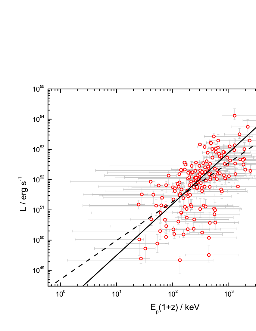
Figure 1.— $L$-$E_{p}$ relationship of the 172 redshift-known Swift GRBs (open circles). The dashed line represents the least-squares fit, while the solid line is obtained by reconciling the distributions of pseudo- and real redshifts.

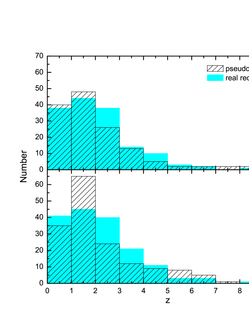
Figure 2.— Comparisons between the number distributions of pseudo- and real redshifts of the redshift-known GRBs. The top panel shows the case where two distributions are closest to each other, while the bottom panel is obtained with the least-squares fit to the $L$-$E_{p}$ relationship.

Until GRB 120811C, in total there were 580 long-duration ($T_{90}>2$ s) GRBs detected by Swift, where 172 GRBs have been measured at redshift. Throughout this Letter, only long-duration GRBs are considered. Additionally, three GRBs with a luminosity $L<10^{49}\rm erg~{}s^{-1}$ have been excluded, because they could belong to a distinct population called low-luminosity GRBs (Soderberg et al. 2004; Liang et al. 2007). For a redshift-known GRB, its luminosity can be calculated by $L=4\pi d_{l}(z)^{2}Pk(z)$, where $d_{l}(z)$ is the luminosity distance, $P$ is the observed peak flux in the Burst Alert Telescope (BAT) energy band 15-150 keV, and $k(z)\equiv\int_{1\rm keV}^{10^{4}\rm keV}S(E^{\prime})E^{\prime}dE^{\prime}/\int_{15(1+z)\rm keV}^{150(1+z)\rm keV}S(E^{\prime})E^{\prime}dE^{\prime}$ (the primes represent rest-frame energy) converts the observed flux into the bolometric flux in the rest-frame 1-$10^{4}$ keV. As is widely accepted, the observed photon number spectrum $S(E)$ can be well expressed by the empirical Band function (Band et al. 1993). Here we take the related data including redshifts, peak fluxes, and spectral peak energies from Butler’s GRB catalog. It should be noted that the peak energies are actually estimated by Bayesian statistics but not directly observed, because the Swift BAT energy bandpass is too narrow. In Figure 1, we plot the 172 redshift-known GRBs in the $L$-$E_{p}$ plane, where a correlation between $L$ and $E_{p}$ appears. Such a correlation was first proposed by Wei & Gao (2003), Liang et al. (2004), and Yonetoku et al. (2004) independently. The least-squares fit to the $L$-$E_{p}$ correlation is shown by the dashed line in Figure 1, which reads

$${L\over 10^{52}{\rm erg~{}s^{-1}}}=A\left[{E_{p}(1+z)\over 1\rm MeV}\right]^{\eta},$$ (1)

with $A=3.47$ and $\eta=1.28$. According to the above equation, a pseudo-redshift in principle can be derived from a pre-obtained peak energy of a Swift GRB. However, in view of the actual dispersion of the $L$-$E_{p}$ relationship, the pseudo-redshift is not expected to precisely equal to the observationally measured one.

Therefore, for a less strict but statistically sound consideration, here we suggest a new criterion for determining the $L$-$E_{p}$ relationship and calculating pseudo-redshifts. Instead of finding sufficiently precise pseudo-redshifts for individual GRBs, we regard all of the redshift-known GRBs as an entire statistical entity and focus on the distribution of pseudo-redshifts. To be specific, first we loosen the $L$-$E_{p}$ relationship by freeing the parameters $A$ and $\eta$ in Equation (1). Then the process of the determination of a pseudo-redshift becomes as follows: (1) to assign a value to the parameters $A$ and $\eta$; (2) to calculate pseudo-redshifts for the 172 redshift-known GRBs from the pre-assumed $L$-$E_{p}$ relationship, where the errors of $E_{p}$ are ignored; (3) to compare the distributions of pseudo- and real redshifts of the 172 redshift-known GRBs with the $\chi^{2}$ test; and (4) to find the most likely values of $A$ and $\eta$ by minimizing the value of $\chi^{2}$. In other words, our purpose is to reduce the discrepancy between the distributions of pseudo- and real redshifts as much as possible. Consequently, we obtain $A=7.93$ and $\eta=1.70$, as shown by the solid line in Figure 1. This is obviously different from the least-squares fit. With such a modified $L$-$E_{p}$ relationship, we finally calculate pseudo-redshifts for 150 redshift-known GRBs, but can not for the remaining 22 ones because their fluxes are too low with respect to their spectral peak energies. Both of the distributions of pseudo- and real redshifts of the 150 redshift-known GRBs are presented in the top panel of Figure 2, while the result corresponding to the least-squares fit is shown in the bottom panel for a comparison.

By extending the modified $L$-$E_{p}$ relationship to all Swift GRBs, 498 GRBs can be assigned a pseudo-redshift, occupying a fraction 86% of total Swift GRBs. Moreover, there are 38 GRBs predicted to be beyond the redshift $z\sim 10$, even at a redshift of a few tens. Optimistically, one may expect to use these GRBs to explore the universe at the beginning of reionization era. Figure 3 shows the 498 GRBs in the $L$-$z$ plane with their error bars reflecting the uncertainties of peak energies of Butler’s catalog with a $90\%$ confidence. Strictly speaking, the errors of a great number of GRBs could be too large for an exact statistics, which makes our following results subjecting to large uncertainty. Anyway, the open circles in Figure 3 representing the most likely parameters of the GRBs seem still to distribute “normally” in the $L$-$z$ plane, by comparing with the $L$-$z$ distribution of redshift-known GRBs (e.g., see Figure 1 in Cao et al. 2011). Therefore, as a perilous attempt, in the following statistics we only take into account the most likely parameters and ignore their error bars.

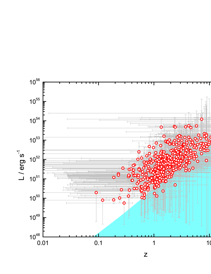
Figure 3.— Luminosity-redshift distribution of 498 GRBs with pseudo-redshifts, where the open circles represent the most likely values and the error bars are determined by the uncertainties of peak energies of Butler’s catalog with a $90\%$ confidence. The shaded region is determined by the lower cutoff luminosity (see Equation (5)).

3. Luminosity function

As the main interest of this Letter, we constrain the GRB LF with the pseudo-redshift-obtained GRBs. In comparison with previous works, this work could have two advantages: (1) the RSEs have been removed, which significantly reduces the uncertainty of the model, and (2) the GRB sample is enlarged by about three times, which makes it possible to provide redshift-resolved luminosity distributions. Our statistics would be restricted to below the redshift $3.5$, because the star formation history above $z\sim 3.5$ is unclear at present (Hopkins & Beacom 2006; Bouwens et al. 2007, 2011; Oesch et al. 2010; Yu et al. 2012; Coe et al. 2012; Tan & Yu 2013). For relatively low redshifts, the star formation history can be described by (Hopkins & Beacom 2006),

$$\dot{\rho}_{\star}(z)\propto\left\{~{}~{}\begin{array}[]{ll}(1+z)^{3.44},&~{}~{}~{}~{}z\leq 0.97,\\ (1+z)^{0},&~{}~{}~{}~{}0.97<z\leq 3.5,\end{array}\right.$$ (4)

with the local star formation rate $\dot{\rho}_{\star}(0)=0.02~{}M_{\odot}\rm yr^{-1}Mpc^{-3}$.

It is natural to consider that the paucity or absence of GRBs in the range of relatively low luminosities as shown by the shaded region in Figure 3 is caused by the multiple thresholds of all related telescopes, especially the Swift BAT. However, because of the very complicated trigger processes of the BAT, it seems impossible to exactly express the BAT threshold. We only know that the trigger probability of the BAT could increase with increasing gamma-ray brightness and eventually approach one. Therefore, in order to avoid the uncertainty arising from the BAT trigger probability, we take a sufficiently high flux $P_{\rm lc}=2\times 10^{-8}~{}\rm erg~{}s^{-1}~{}cm^{-2}$ as the lower cutoff of peak flux for our statistics. Above $P_{\rm lc}$, the trigger probability can basically be considered to unity. The corresponding lower cutoff luminosity, which is shown by the upper boundary of the shaded region in Figure 3, can be calculated by

$$L_{\rm lc}(z)=4\pi d_{L}(z)^{2}P_{\rm lc}k(z),$$ (5)

where the $k$-correction factor is calculated with a typical (averaged) rest-frame peak energy $E^{\prime}_{p}\sim 150~{}\rm keV$. As a result, 17 GRBs with $L<L_{\rm lc}$ are excluded and 361 GRBs remain.

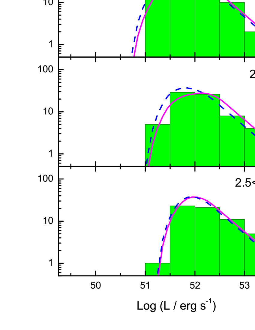
Figure 4.— Distributions of GRB numbers in different luminosity bins for different redshift intervals as labeled. Fittings to the luminosity distributions with a constant and an evolving LF are presented by the dashed and solid lines, respectively. Note that the GRB numbers presented here are actually counted with large uncertainties of the luminosities, as indicated in Figure 3, which are, however, not displayed for simplicity.

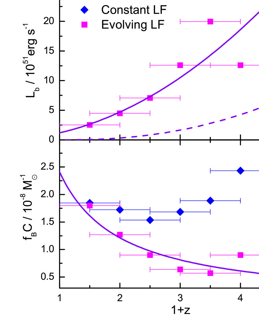
Figure 5.— Redshift-dependences of parameters $L_{b}$ and $f_{B}C$ in both constant and evolving LF cases, where the horizon error bars represent the width of the redshift intervals. The errors of the parameter values could be very large but not displayed due to the difficulty of the error estimation. In the evolving LF case, two empirical power-law fittings are provided by the solid lines. The adopted lower cutoff luminosity is presented by the dashed line in the top panel for a comparison.

In view of the relatively large number of the remaining GRBs, we divide the adopted GRB sample into six redshift intervals as $0<z<1$, $0.5<z<1.5$, $1<z<2$, $1.5<z<2.5$, $2<z<3$, and $2.5<z<3.5$. The adjacent intervals are taken to overlap with each other just in order to obtain a sufficiently large GRB number for each redshift interval. Then, from the second to seventh top panels in Figure 4, we display the corresponding redshift-resolved luminosity distributions independently, and meanwhile the combined distribution of all redshift ranges is presented in the first top panel. In the theoretical aspect, the GRB number within the luminosity bin $L_{1}<L<L_{2}$ for a redshift interval $z_{1}<z<z_{2}$ can be calculated by

$$N = {\Delta\Omega\over 4\pi}T\int^{z_{2}}_{z_{1}}\int^{L_{2}}_{\max[L_{1},L_{\rm lc}(z)]}\Phi_{z}(L)\dot{R}(z)dL{dV(z)\over 1+z},$$ (6)

where $(\Delta\Omega/4\pi)\sim 0.1$ is the field view of the BAT, $T\sim 7\rm yr$ the observational period, and $dV(z)$ the comoving volume. The observational GRB production rate can be connected to star formation rate as

$$\dot{R}(z)=f_{B}C~{}\dot{\rho}_{\star}(z),$$ (7)

where $f_{B}$ is the beaming degree of GRB outflows and the proportional coefficient $C$ could arise from the particularities of GRB progenitors (e.g., mass, metallicity, magnetic field, etc). For the LF $\Phi_{z}(L)$, two popular competitive forms, including the broken-power law and the single-power law with an exponential cutoff at low luminosity, are tested in Cao et al. (2011). As a result, the broken-power-law LF as

$$\Phi_{z}(L)\propto\left\{~{}\begin{array}[]{ll}\left({L\over L_{b}(z)}\right)^{-v_{1}},{}{}{}{}&L\leq L_{b}(z),\\ \left({L\over L_{b}(z)}\right)^{-v_{2}},{}{}{}{}&L>L_{b}(z),\end{array}\right.$$ (10)

is suggested to be more consistent with observations. The normalization coefficient of the LF is taken with an assumed minimum luminosity $L_{\min}=10^{49}\rm~{}erg~{}s^{-1}$. To summarize, for a fitting to a GRB luminosity distribution, we need to determine values for four model parameters as $f_{B}C$, $L_{b}$, $\nu_{1}$, and $\nu_{2}$.

For a general consideration, here we fit the GRB luminosity distributions in two different ways, i.e., with a constant and an evolving LF, which are presented by the dashed and solid lines in Figure 4, respectively. In both cases, the values of $\nu_{1}$ and $\nu_{2}$ are considered to be constant. As suggested in Cao et al. (2011), the value of the high-luminosity index $\nu_{2}$ could be found directly from the distribution of high-luminosity GRBs, because the telescope thresholds nearly cannot affect the detection of these GRBs. Then we get $\nu_{2}=2.0$, which is the same as that in Cao et al. (2011). Subsequently, (1) with a constant LF assumption, we constrain the model parameters by fitting the combined luminosity distribution of all GRBs, which gives rise to the best-fitting parameters $L_{b}=1.3\times 10^{52}$ and $\nu_{1}=1.2$. With the determined $L_{p}$, $\nu_{1}$, and $\nu_{2}$, we further fit the six redshift-resolved luminosity distributions to find the best-fitting values of $f_{B}C$ in different redshift ranges. The results are presented in the bottom panel of Figure (diamonds), where the last data at $1+z=4$ lead us to see an increase of $f_{B}C$ with increasing redshift. This is qualitatively consistent with previous findings of the evolution effect (e.g., Kistler et al. 2009). However, if we remove the last data, the redshift-dependence of $f_{B}C$ could become ambiguous or, at least, very weak. (2) In the evolving LF model, we should fit the six redshift-resolved luminosity distributions independently rather than with a predetermined $L_{p}$. The best-fitting values of $L_{p}$ and $f_{B}C$ for different redshifts are also presented in Figure 5 (squares). The constant low-luminosity index is simultaneously determined to $\nu_{1}=0.8$. As shown by the solid lines in Figure 5, on the one hand, an obvious evolution of the break luminosity $L_{b}$ appears as

$$L_{b} = 1.2\times 10^{51}(1+z)^{2}~{}\rm erg~{}s^{-1},$$ (11)

which is qualitatively consistent with the result in Yonetoku et al. (2004) for BATSE GRBs. Moreover, the difference between the redshift dependences of $L_{b}(z)$ and $L_{\rm lc}(z)$ suggests that the evolution of the LF is probably intrinsic rather than observational. Such an LF evolution indicates that higher-redshift GRBs could be much brighter than the lower-redshift ones. On the other hand, the coefficient $f_{B}C$ is found to decrease with increasing redshift as

$$f_{B}C = 2.4\times 10^{-8}(1+z)^{-1}M_{\odot}^{-1},$$ (12)

which is completely opposite to that of the previous understanding with a constant LF.

Finally, Figure 4 shows that both the constant and evolving LF models can provide a perfect fitting to the combined luminosity distribution of all GRBs. In other words, it is impossible to distinguish the two models by the combined distribution. However, for the six redshift-resolved luminosity distributions, it is clearly shown that the fittings with an evolving LF are always better than the ones with a constant LF, in particular, for relatively low redshifts. Therefore, we prefer to conclude that an evolving LF is more favored by the pseudo-redshift GRB sample.

4. Summary and discussions

In view of their association with Type Ib/c supernovae and the bright gamma-ray emission (Stanek et al. 2003; Hjorth et al. 2003; Chornock et al. 2010), GRBs are usually suggested to trace the cosmic star formation history. However, due to the thresholds of telescopes, the conversion from the GRB event rate to star formation rate is strongly dependent on the form of the LF, and moreover the determination of the LF is seriously hindered by the RSEs. One viable method is to take only the high-luminosity GRBs into account, as was done in Kistler et al. (2009) and Wang & Dai (2011). Such a method could become invalid if the LF is redshift-dependent. Alternatively, in this Letter, we suggest to use an empirical GRB relationship (i.e., $L$-$E_{p}$ relationship) to calculate pseudo-redshifts for Swift GRBs, so that the RSEs can be avoided in the new redshift sample. In view of the insufficient tightness of the adopted $L$-$E_{p}$ relationship, we replace the least-squares fit to the relationship by a modified one with which the distribution of the pseudo-redshifts can be closest to the observational one. Consequently, a GRB sample of a large number is obtained, which makes it possible to analyze the GRB luminosity distributions in different redshift ranges. As found by Yonetoku et al. (2004) for BATSE GRBs, here we also find the LF of Swift GRBs could evolve with redshift by a redshift-dependent break luminosity $L_{b}$. Such an evolving LF also changes our understanding of the intrinsic connection between the GRBs and stars, i.e., the parameter $f_{B}C$ should decrease (but not increase as previously considered) with increasing redshifts. In other words, both the GRB production efficiency and the luminosities of the produced GRBs should be very different at different cosmic times, which may provide some new constraints on the properties of GRB progenitors and central engines.

References

- (1) Amati, L., Frontera, F., Tavani, M., et al. 2002, A&A, 390, 81
- (2) Band, D., Matteson, J. Ford, L. et al. 1993, ApJ, 413, 281
- (3) Band, D. L. 2003, ApJ, 588, 945
- (4) Bouwens, R. J., Illingworth, G. D., Franx, M., & Ford, H. 2007, ApJ, 670, 928
- (5) Bouwens, R. J., Illingworth, G. D., Labbe, I., et al. 2011, Natur, 469, 504
- (6) Bromm, V., & Loeb, A. 2006, ApJ, 642, 382
- (7) Butler, N. R., Bloom, J. S., & Poznanski, D. 2010, ApJ, 711, 495
- (8) Butler, N. R., Kocevski, D., Bloom, J. S., & Curtis, J. L. 2007, ApJ, 671, 656
- (9) Campisi, M. A., Li, L.-X., & Jakobsson, P. 2010, MNRAS,407, 1972
- (10) Cao, X. F., Yu, Y. W., Cheng, K. S., & Zheng, X. P. 2011, MNRAS, 416, 2174
- (11) Chornock, R., Berger, E., Levesque, E. M., et al. 2010, ApJL, submitted (arXiv:1004.2262)
- (12) Coe, D., Umetsu, K., Zitrin, A., et al. 2012, ApJ, 757, 22
- (13) Coward, D.M., Howell1, E. J., Branchesiet, M., et al. 2012, arXiv: 1210.2488
- (14) Cucchiara, A., Levan, A. J., Fox, D. B., et al. 2011, ApJ, 736, 7
- (15) Daigne, F., Rossi, E. M., & Mochkovitch, R. 2006, MNRAS, 372, 1034
- (16) de Souza, R. S., Yoshida, N., & Ioka, K. 2011, A&A, 533, 32
- (17) Ghirlanda, G., Ghisellini, G., & Lazzati, D. 2004, ApJ, 616, 331
- (18) Greiner J., Bornemann, W., Clemens, C., et al. 2008, PASP, 120, 405 2004, ApJ, 615, L73
- (19) Hjorth, J., Sollerman, J., Møller, P., et al. 2003, Natur, 423, 847
- (20) Hopkins, A. M., & Beacom, J. F. 2006, ApJ, 651, 142
- (21) Jakobsson, P., Hjorth, J., Fynbo, J. P. U., et al. 2004, A&A, 427, 785
- (22) Kistler, M. D., Yksel, H., Beacom, J. F., et al. 2009, ApJL, 705, L104
- (23) Levan, A., Fruchter, A., Rhoads, J., et al. 2006, ApJ, 647, 471
- (24) Liang, E. W., Dai, Z. G., & Wu, X. F. 2004, ApJL, 606, L29
- (25) Liang, E. W., & Zhang, B. 2005, ApJ, 633, 611
- (26) Liang, E. W., Zhang, B., Virgili, F., & Dai, Z. G. 2007, ApJ, 662, 1111
- (27) Lloyd-Ronning, N. M., Fryer, C. L., & Ramirez-Ruiz, E. 2002, ApJ, 574, 554
- (28) Murakami, T., Yonetoku, D., Izawa, H., & Ioka, K. 2003, PASJ, 55, L65
- (29) Natarajan, P., Albanna, B., Hjorth, J., et al. 2005, MNRAS, 364, L8
- (30) Oesch, P. A., Bouwens, R., J., Illingworth, G. D., et al. 2010, ApJL, 709, L16
- (31) Salvaterra, R., & Chincarini, G. 2007, ApJL, 656, L49
- (32) Salvaterra, R., Guidorzi, C., Campana, S., Chincarini, G., & Tagliaferri, G. 2009, MNRAS, 396, 299
- (33) Salvaterra, R., Campana, S., Vergani, S. D., et al. 2012, ApJ, 749, 68
- (34) Soderberg, A. M., Kulkarni, S. R., Berger, E., et al. 2004, Natur, 430, 648
- (35) Stanek, K. Z., Matheson, T., Garnavich, P. M., et al. 2003, ApJH, 591, L17
- (36) Steidel, C., Shapley, A., Pettini, M., et al. 2005, in Proc. ESO Workshop in Venice, Italy, 13-16 October 2003, Multiwavelength Mapping of Galaxy Formation and Evolution, ed. A. Renzini and R. Bender (Berlin: Springer) 169
- (37) Tan, W. W., Yu, Y. W. 2013, Sci. China Phys. Mech. Astron., 56, 1029
- (38) Wanderman, D., & Piran, T. 2010, MNRAS, 406, 1944
- (39) Wang, F. Y., & Dai, Z. G. 2011, ApJL, 727, L34
- (40) Wei, D. M., & Gao, W. H. 2003, MNRAS, 345, 743
- (41) Yonetoku, D., Murakami, T., Nakamura, T., et al. 2004, ApJ, 609, 935
- (42) Yu, Y. W., Cheng, K. S., Chu, M. C., & Yeung, S. 2012, JCAP, 07, 023