Phase Transition in the S&P Stock Market
Abstract
We analyze the returns of stocks contained in the Standard & Poor’s 500 index from 1987 until 2011. We use covariance matrices of the firms’ returns determined in a time windows of several years. We find that the eigenvector belonging to the leading eigenvalue (the market) exhibits a phase transition. The market is in an ordered state from 1995 to 2005 and in a disordered state after 2005. We can relate this transition to an order parameter derived from the stocks’ beta and the trading volume. This order parameter can also be interpreted within an agent-based model.
The final publication is available at link.springer.com
http://link.springer.com/article/10.1007/s11403-015-0160-x
to be published in the Journal of Economic Interaction and Coordination.
1 Introduction
In this paper we analyze the structure of the U.S. stock market. We show that the influence of stocks on the market is changing and that this influence is related to trading volume and the stocks’ betas.
The analysis of the structure of stock markets is dominated by two research approaches. The first one tries to explain the differences between the rates of return of stocks and relates to the seminal work by Lintner (1965) and Sharpe (1964) and the CAPM model. The second approach takes the investor’s point of view, and is hence mostly focused on the choice of a portfolio and the analysis of risk. Both are related by the need to evaluate the comovement of stocks with each other and some index or market proxy.
The original version of the CAPM is in fact a one-factor-model, which postulates that the returns of the stocks should be governed by the market return and only differ by the an idiosyncratic component for each stock , such that
| (1) |
In this setting can also be interpreted as the risk free rate of interest. Hence, stocks differ by the amount of volatility with respect to the market, and economic rationale necessitates that higher stock volatility is compensated by higher absolute returns. Empirical tests of this model had rather mixed results and have let to the conclusion that beta values are not constant but time-varying, see Bollerslev et al. (1988). The Fama and French (1992) model extends this approach to a three-factor model, incorporating firm size and book-to-market ratio. Several other extension of the original models have been suggested, mostly building on some kind of conditional CAPM, where the entire model follows a first-order auto-regressive process, see Bodurtha and Mark (1991). The reasons for the change of the betas are manifold. They could change due to microeconomic factors, the business environment, macroeconomic factors, or due to changes of expectations, see, e.g., Bos and Newbold (1991). Adcock et al. (2012), Harvey and Siddique (2000) and Plerou et al. (2002) have discussed that the non-normality of stock returns, conditional skewness, and mainly the long memory in returns can lead to distorted estimations of the CAPM. There is also a strand of literature that tries to capture the effects of heterogeneous beliefs of investors in a CAPM framework, e.g., Brock and Hommes (1998) and Chiarella et al. (2010).
In order to manage the risk of a portfolio, one can derive optimal portfolio weights from the spectral decomposition of the covariance matrix of stock returns. Many studies show that the non-normality of stock returns can lead to an under-estimation of risk. A common way to describe the properties of stock comovements is to look at the eigenvalue spectrum of the correlation matrix. Random matrix theory suggests that a market that behaves like a one-factor model should result in one dominant eigenvalue. Both, the non-normality in the data and any influence from other factors will result in deviations from this simplified model, see Citeau et al. (2001) and Livan et al. (2011).
Approaches which utilize the spectral properties of correlations matrices have their limits once the number of variables becomes large relative to the number of observations. Networks approaches, which derive dependency networks from the correlation matrix can be useful, as long as one does not need explicit portfolio weights for each single stock, see, e.g., Kenett et al. (2012a) and Tumminello et al. (2005). A related approach is to try to identify different states of the stock market, either by an analysis of the correlation matrix like in Münnix et al. (2012), or by the analysis of transaction volumes as in Preis et al. (2011). Recent studies like Kenett et al. (2012b) show that the correlation structure in stock markets are rather volatile, and partly mirror economic and political changes. Kenett et al. (2011) for example shows that a structural break seems to happen in the U.S. market around 2001. This strand of literature is also related to approaches from econometrics. Beile and Candelon (2011) for example argue that correlations increase in times of crisis, which has profound implication for portfolio choice and hedging of risks. Other studies like Ahlgren and Antell (2010) analyze if correlations in and between markets have increased due to more openness and tighter economic relations between countries.
Since financial markets tend to react very fast on any change in the economy, but also inhibit a lot of noise, we found that a look at longer time horizons is a worthwhile contribution to the field, since many of the above mentioned studies look at time horizons of months or a few years. We found that the S&P 500 contains around 170 stocks with a history of price quotes of 25 years (the number drops rapidly with much more than this 25 years). We analyze the long-run development of the stocks influence upon the market. We derive both, a market index and the stocks’ influence, from the spectral decomposition of the covariance matrix. We show that for most of the period under consideration the market was in a ordered state, characterized by a disproportionate influence of stocks from the IT sector. While some changes in the market seem to happen in 1995, the collapse of this regime starts with the burst of the dot.com bubble. A disordered state is found after 2005. We will show that from here the market develops into a new (although weaker) ordered state, where the driving sector is the financial industry.
The paper is organized in the following way. In section 2 we describe the subset of stocks in the S&P market used in this analysis. Section 3 contains the definition of market indices derived from the covariance matrix. In section 4 we explain why we prefer the latter over the usually applied correlation matrix, and that the average return and market return may be almost equal when calculated from a large number of stocks. Section 5 contains our results for the phase transition and section 6 some conclusions.
2 Materials and Methods
The most important criterion for data selection consists in the length of the time series of stock prices. Only 289 firms in the S&P 500 are listed from from January 1987 until December 2011, but not all of them will qualify for our analysis. In the present work we study the covariance matrix of firm returns. To a large part this matrix is a random matrix, where the errors of the quantities of interest are in the order of , see also Marĉenko and Pastur (1967). Therefore one can in fact afford a reduction of by the following criteria: We start out with the 500 stocks which are listed as part of the S&P500 index at the end of 2011. We drop all those which were not trading since January 1987. We then filter for illiquid stocks; we define stocks as illiquid if their price does not change for more than 7% of the trading days. We validate this selection by checking the daily trading volumes. Further we delete single stocks which price does not move for at least 10 days in a row (e.g. due to suspended trading).
Our final set of data comprises the stock prices of firms at trading days in the time window 1987-2011. As a sign of the different sizes of the firms we will later also consider the yearly trading volume of the firms in this period. A disadvantage of our selection consists in the loss of the meaning of the index, since this refers to a changing set of 500 firms and may not be representative for our subset. This selection also leads to some form of selection bias, since failed enterprises are excluded from the analysis.
A frequently used tool to analyze financial markets consists in the study of the correlation matrix between the stock returns of a market. This matrix can be used in two ways. Its observation needs a certain time window . For small window sizes (10-20 days in case of daily returns), the matrix is dominated by noise and a principal component analysis does not make any sense. In the first class of studies like Borland and Hassid (2010) and Kenett et al. (2011), the noise is reduced by averaging the correlation matrix over the stocks. This means to replace the volatility of the average return by the sum of firm returns.
On the other side, when choosing in the order of a few years, the decomposition into eigenvectors may be meaningful. The correlation matrix possesses one large eigenvalue in the order of the number of stocks. The corresponding eigenvector can be used as a description of the market, see Laloux et al. (1999); Galluccio et al. (1998). The remaining eigenvalues are qualitatively similar to those of a random matrix with a Marĉenko and Pastur (1967) spectrum. Nevertheless, with the assumption of a specific model, information can be extracted from this part of the spectrum, see Livan et al. (2011). In general, only eigenvalues separated by more than from other values have a model independent meaning, see Burda et al. (2004). Therefore we concentrate on the long term time behavior of the eigenvector of the market eigenvalue.111Extending the window too much could in fact at some point lead to problems, even if one assumes that the betas are slowly varying, see for example Livan et al. (2012).
A daily market return can be obtained by the scalar product of the stock returns with the eigenvector, determined in an appropriate window. In this case the eigenvector denoted by (normalized to ) describes the coefficients relative to the market, as needed for a CAPM portfolio in the style of Black et al. (1972). This interpretation is supported by the empirical results of Laloux et al. (1999), the are positive and and distributed around one for y.
In an alternative description of the market, the average return may be used, see Borland and Hassid (2010) and Kenett et al. (2011). First, we investigate how much and the index return differ from each other. Secondly we will investigate the time dependence of to find evidence for a phase transition.
Transitions in physics are characterized by an order parameter , which vanishes in the disordered phase and is non-zero in the ordered phase. could be related to macroscopic or microscopic properties of the system. In general, is discontinuous at the critical point (first order). In special cases, the transition is of continuous order with continuous . Corresponding models of statistical physics near the critical region have been applied to financial markets in Cont and Bouchaud (2000); Stauffer and Sornette (1999); Bornholdt (2001). They offer an explanation of the stylized facts of the returns, see Lux and Ausloos (2002). However, due to the universality, the relation of the model parameters to economical quantities remains obscure. The models require fine tuning of the parameters to maintain the system close to the critical region. Since these systems always stay in a disordered phase, neither a micro- nor macroeconomic order parameter can be observed directly. In this study we look for a first order transition of stocks that are characterized by high volatility () and a high trading volume, which we capture by calculating a macroeconomic order parameter .
3 Correlation Matrix and Pseudo Indices
3.1 Properties of the correlation matrix
The daily stock stock prices for stock at day may be converted into returns by
| (2) |
We use a normalization factor given by . To see the time dependence of the correlation between stocks we construct the covariance matrix at time by selecting a time window222In this paper is used to specific days, while is used to index variables like that are calculated for a time window. of size centered at
| (3) |
Many previous investigations (as discussed in the introduction) use the Pearson correlation (Pearson, 1885), which describes the covariance between standardized returns. Subtracting from each time series the mean of would be a small effect, but setting the variance to 1 may mask a possible dependence of the eigenvalues of . For large window sizes has one large eigenvalue of order and the corresponding eigenvector has only positive components, see, e.g., Plerou et al. (2002). Empirically we found that these properties are lost for window sizes less than 3 years. Therefore we will in the following use a window sizes years. To compensate for the loss of time resolution we use overlapping bins by choosing time steps in less than .
The matrix can be written in a spectral decomposition as
| (4) |
where denotes the eigenvalues and the eigenvectors of . The large eigenvalue corresponding to and its eigenvector can be interpreted as a description of the market, see, e.g., Plerou et al. (2002). It can be used to define a market return for in a window
| (5) |
This means that the market return (which is also a market index) consists of the weighted contributions of the returns of the single stocks. The weights are proportional to the entries in the eigenvector that corresponds to the leading eigenvalue.
For the CAPM model, one needs so-called -coefficients, which describe how close a stock follows the market described by a reference return .
| (6) |
In a dynamic analysis the vector of beta values becomes time dependent. For our analysis we calculate betas in time windows . As a reference return we use the market return instead of the real S&P-index, because the latter may not be representative for our data selection. Replacing the expectation values in equation 6 by taking time averages we obtain with from equation 4 the following coefficients
| (7) |
After resolving the sign ambiguity in we recover the fact that for years all are positive. Due to the normalization the are distributed around a mean close to 1. Firms with large follow the market more than others and also they influence the market more than firms with small . For this reason we will refer to stocks with larger than a given threshold as the market leaders.
3.2 The market
A simple way of defining a market would be the average return
| (8) |
averaged over time corresponds to a correlation matrix, averaged over the stocks, which has also its defenders in the literature, see Borland and Hassid (2010); Kenett et al. (2011). From the returns defined by equation (8) we can calculate logarithms of a pseudo index by the recursion
| (9) |
The market return from equation (5) refers to a specific window. To define a market pseudo index we use which is defined for all by equation (5) with of the window with center next to .
| (10) |
The recursions (9) and (10) can be integrated. The integration constants are fixed by the normalization
| (11) |
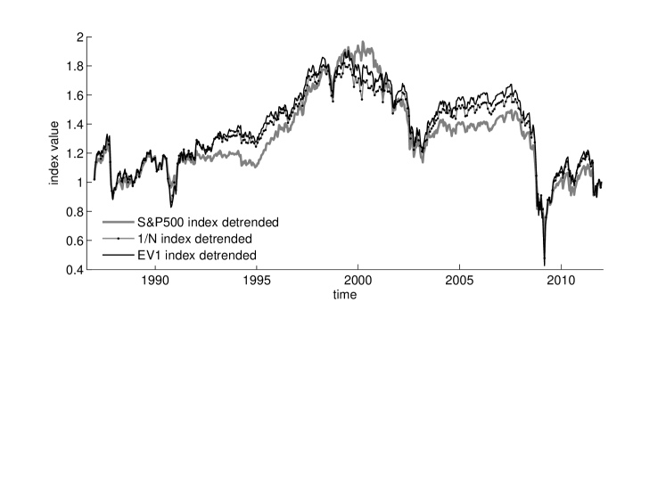
We compare these pseudo indices in figure 1 with the index , written in the form . ensures equation (11) also for . As expected, the market index calculated with a time window of years agrees with only qualitatively. The average pseudo index is very similar to the market pseudo index . This is somewhat surprising since we will see that can change with time. Especially in the years 2001-2008 the index exhibits considerably larger average returns than the pseudo indices. This effect can be interpreted as phase transition into a stiff market. It was detected in Kenett et al. (2011), where correlations with the index have been subtracted from the stock correlations. An increase of the former correlation leads to smaller subtracted correlations after 2001.
For the squared difference of and given by
| (12) |
we derive in appendix A the inequality
| (13) |
with the mean of . The average correlation
| (14) |
can be expressed by and the properties of the market component (see appendix A) up to terms of order
| (15) |
In the next section we discuss that for large markets () both, empirically and in context of a model, approaches one and therefore vanishes. In this limit corresponds to the volatility of the market.
4 Dependence on the Market Size
The qualitative behavior of the correlation matrix suggests a decomposition of the returns according to a stochastic volatility model, see Cont (2001). is the sum of the two products, of noise and the market and of noise and the remaining contribution. The coefficients , the coupling to the market, and the idiosyncratic couplings are assumed to be constant in each window.
| (16) |
The independent noise factors have mean 0 and variance 1. The coefficients are normalized to . For can be determined from the expectation values
| (17) |
For large one can solve the eigenvalue problem for by a expansion (see appendix B). has one large eigenvalue
| (18) |
with an eigenvector corresponding to
| (19) |
denotes an average over .

Neglected terms in equations (18) and (19) are of order . Empirically the are distributed around a mean close to 1 and a variance decreasing with . Therefor, we can assume the model parameter to be equal to one. From the inequality (13) we see that the difference between and expressed by (see equation (12)) has to vanish in this limit.
In the following we investigate the behavior of the leading eigenvalue , and as function of .
A finite window size leads to deviations of the observed from the ideal of equation (17) in the order of . To minimize this systematic error, we choose the maximum window size . To have a varying we adopt the following procedure: Sub-markets are defined by dividing the stocks into groups with size such that each group contains the same fraction of large and small firms as the full set. To improve the statistics we average , and over the groups. The result is presented in figure 2, which shows these quantities as a function of on a log-log scale. (dashed dotted line) increases with with a power of close to 1. (solid line) and (dashed line) exhibit a lesser decrease than the expected behavior. Since they also flatten out at large , this indicates an influence of the finite observation time window. The observed values of are much smaller than the upper limit from the Schwartz inequality in equation (13). This indicates that the eigenvectors for are almost orthogonal to a constant vector already at finite , which implies equality of and .
To summarize, the data support a stochastic volatility model of a sum of market and preferences for individual stocks where for large the stock returns couple to the market component in the same way. Therefore can be taken as a description of the market. Since it determines the average correlation , the frequent use of in the literature as a proxy for an index is empirically successful. Especially consists in a good estimator for the leading eigenvalue , since due to the law of large numbers the statistical error decreases with both, and . From the perturbation expansion given in appendix B we see that the leading eigenvalue and its vector can be more accurately determined than the remaining ones.
5 Time Dependence of and Phase Transition
In the previous section the coefficients and have been discussed for a long time scale. In general however, they will be time dependent. To minimize the influence of the noise produced by a finite observation window , we chose a rather large window of years. This implies that only long term changes in can be detected. In the following, we diagonalize for the S&P data in overlapping steps of 1 year.


The resulting time dependence of is shown in figure 4 for the 60 firms with the smallest average traded volume. Before 2005, their beta values are relatively constant with values , as expected for small firms with less impact on the market. Around 2005 some firms with previously small experience a drastic increase and become market leaders (firms with are indicated by solid lines). A different picture appears if we look at for firms with large average traded volume shown in figure 4 for the 60 largest firms. Of course this set contains market leaders. Those in 2002 are denoted by solid lines. However, in 2005 they disappear in favor of new firms as in the case of small firms. Therefore in 2005 a reorganization of the market has happened. This depends on the the sector classification of the firms. The 18 market leaders in the set of all firms with in the year 2002 are listed in table 3 and in table 3 those for the year 2008. The 2002 list contains dominantly large firms from the IT sector. After the transition in 2008 the list contains firms of all sizes spread over many sectors.
| Sector name | # in sample | Sector name | # in sample |
|---|---|---|---|
| Consumer Discretionary | 24 | Consumer Staples | 22 |
| Energy | 10 | Financials | 28 |
| Health Care | 18 | Industrials | 33 |
| IT | 20 | Materials | 14 |
| Telecommunication Services | 3 | Utilities | 0 |
This behavior of might indicate a phase transition. A macroeconomic order parameter that explains this transition should take into account the (large) values, the traded volume (see also (Dichev et al., 2012)) and the sectors of the firms. For we use the GICS classification scheme into sectors given in table 1. From the point of view of an investor, one can say that the following function describes the risk (volatility) in each sector due to the coefficients
| (20) |
In an ordered state one specific is large and the remaining ’s are small. A macroeconomic order parameter of a Potts model type can be obtained by normalizing
| (21) |
If the appearance of one large is due to a transition to an ordered state, will be close to 1 and the ’wrong’ order parameters for will scatter around small negative values due to the analogue of thermal fluctuations. In the disordered phase all will fluctuate around 0.
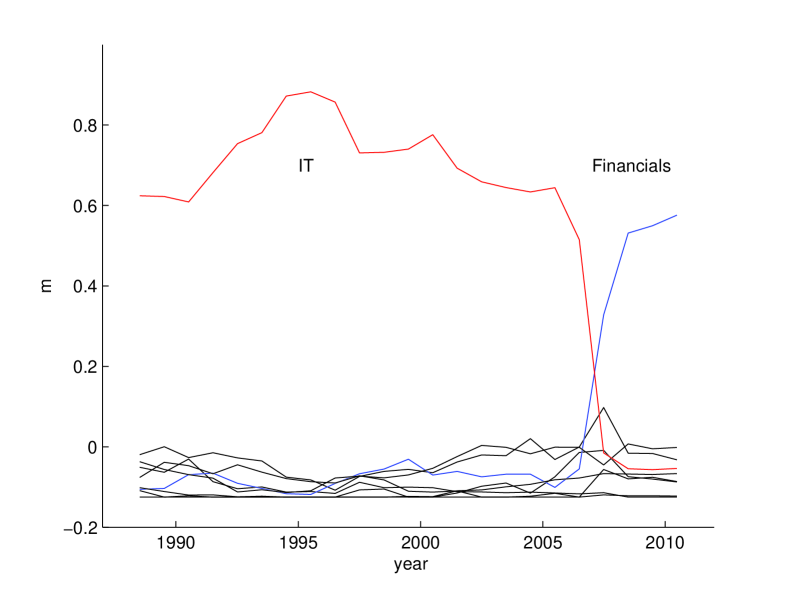
In figure 5 we show the order parameters in time steps of one year. Clearly is large for the IT sector, whereas all others are small negative. After 2006 decreases. Near the end of our time series an ordering towards the financial sector may be possible. 333The dominance of the IT sector and the change around 2005 can also be found for smaller window sizes of down to 2 years, revealing one sharp peak around 1995/96. For much smaller time windows the influence of single events like the 1987 stock market crash or the 9/11 attacks become rather large and distort long-run trends. Following the advice of an unknown referee we discuss in appendix C that the effect seen in figure 5 is not due to the change of only a few firms.
| Firm | Sector | Vol. | Firm | Sector | Vol. | ||
|---|---|---|---|---|---|---|---|
| TEXAS I. | IT | 2.21 | 2966 | HALLIBURTON | Energy | 2.09 | 2641 |
| ALTRIA | Cons. S. | 2.04 | 8927 | BANK OF A. | Finance | 1.94 | 3254 |
| HEWLETT-P. | IT | 1.89 | 2883 | MICROSOFT | IT | 1.87 | 19418 |
| APPLIED M. | IT | 1.69 | 6735 | AM. EXP. | Finance | 1.69 | 1478 |
| ORACLE | IT | 1.66 | 11797 | INTEL | IT | 1.66 | 14429 |
| PFIZER | Health | 1.54 | 4272 | ADOBE | IT | 1.53 | 1886 |
| LOWE’S | Cons. D. | 1.51 | 2511 | JOHNSON & J. | Health | 1.50 | 2079 |
| HERSHEY | Cons. S. | 1.44 | 422 | MERCK | Health | 1.40 | 1884 |
| APPLE | IT | 1.39 | 18540 | INTERN.BUS. | Industry | 1.39 | 2347 |
| Firm | Sector | Vol. | Firm | Sector | Vol. | ||
|---|---|---|---|---|---|---|---|
| HUMANA | Health | 2.11 | 828 | INTERN.BUS. | Industry | 1.86 | 2379 |
| WEYERH. | Finance | 1.86 | 1623 | CHUBB | Finance | 1.80 | 914 |
| VARIAN | Health | 1.64 | 367 | TEXTRON | Industry | 1.63 | 873 |
| CHEVRON | Energy | 1.63 | 3923 | DONNELLEY | Industry | 1.60 | 412 |
| A. DATA | Industry | 1.55 | 823 | TARGET | Cons. D. | 1.51 | 3191 |
| LOWE’S | Cons. D. | 1.46 | 3893 | C R BARD | Health | 1.45 | 211 |
| AVON | Cons. S. | 1.45 | 1098 | MICROSOFT | IT | 1.44 | 21314 |
| G. PARTS | Cons. D. | 1.44 | 309 | PROG. OHIO | Finance | 1.41 | 1461 |
| CIGNA | Health | 1.39 | 918 | WASH. PST. | Cons. D. | 1.39 | 8 |
There are different possibilities to relate this phase transition to the behavior of agents that trade in this market. A microeconomic order parameter could be obtained by incorporating a behavioral agent-based model for the market of the Kirman (1993) type. The sector specific returns could be defined as
| (22) |
like in Alfarano et al. (2005) or Wagner (2006). is proportional to the ratio of noise traders and fundamentalist agents that trade stocks in sector . The i.i.d. Gaussian noise describes the noise traders. is (on a longer time scale) time dependent, because the opinion of the agents changes. With suitable choice of the parameters in the asymmetric Kirman model (see Alfarano et al. (2005) using the bimodal version) this ratio can occasionally be large, and the system stays in this state for longer times. Such a situation cannot be distinguished empirically from a real phase transition. A microeconomic order parameter related to the herding effect would then be given by
| (23) |
An alternative model is the application of a Pott’s model with states, see Wu (1982). The dependent interaction between agents is attractive if neighboring agents trade in the same sector. For strong enough dependent interactions the system will order, with one sector dominating the others.
6 Conclusions
Our analysis of the market indices revealed that for a sufficiently large samples of stocks and longer time horizons weighted indices differ only very slightly from any form of market average. This is a result of strong overall stock correlations and relatively stable long-run correlation structures that we have shown by the analysis of the properties of the correlations matrix.
In our analysis of how the market is influenced by different stocks in the long-run, we have seen that the IT sector has played a dominant role for a long time. The time dependence of the CAPM coefficients exhibit a transition in 2005. This is connected with the disappearance of a macroeconomic order parameter for the IT sector. Despite our poor time resolution due to the window size, this phase transition appears to be sharp. The transition lies between the crash of the dot.com bubble and the Lehmann desaster in 2008. In this time period we see no other pronounced effect in the index or in the stock prices.
A possible reason for a sharp transition may be the following: From 1990 to 2002 the stock prices experienced a steady increase. This led investors to buy in the most increasing sector, the IT sector. They minimized the risk by choosing only large firms. Disappointed by the crash of the dot.com bubble in 2001, they changed their investment strategy completely. Investments and trading volume became much more scattered over all segments. Figure 5 shows that later a (weaker) form of ordering took place by focusing on the financial sector.
Appendix
Appendix A Correlation Matrix
Denoting the time average as in equation (3) by we get from equations (4) and (5) the average of
| (24) |
Similarity we get for and
| (25) |
with
| (26) |
corresponds to the mean value of over .
| (27) |
Inserting equations (24), (25) and (27) into from (4) we get
| (28) |
Since and are orthogonal for we can write as
| (29) |
Applying the Schwartz inequality to (29) we get
| (30) |
Together with this leads to the inequality (13) for . Since the average is a function insertion of into equation (25) leads to equation (15).
Appendix B Perturbation Expansion
The matrix in equation (17) is a sum of two matrices. The first has one large eigenvalue with an eigenvector and degenerate zero eigenvalues with vectors with .These must satisfy only the orthogonality relation
| (31) |
with ( denoting the scalar product. To obtain a complete basis we impose on in the dimensional subspace the following conditions with the second matrix
| (32) |
We apply standard second order Rayleigh Schrödinger perturbation theory 444See any textbook on quantum mechanics, e.g., Messiah (1967). with as perturbation. For general matrices and using only the spectrum of and condition (31) we get up to order for the leading eigenvalue
| (33) |
and its eigenvector
| (34) |
The other eigenvalues require the in general complicated solution of equation (17) for . They are given by
| (35) |
Inserting the specific form of we obtain for and with
| (36) |
| (37) |
| (38) |
| (39) |
denotes the average over weighted with . Since neglected terms are of order these formulae describe and fairly accurate already for moderate . Due to the degeneracy the general formalism of Marĉenko and Pastur (1967) for the modification due to noise does not apply. Using the Wishart (1928) formula we find the relative error in due to a finite observation window is of order instead of expected from Marĉenko and Pastur (1967) . The non-leading eigenvalue will be changed considerably if the spread of is small, see Burda et al. (2004).
Appendix C Significance of the order parameter
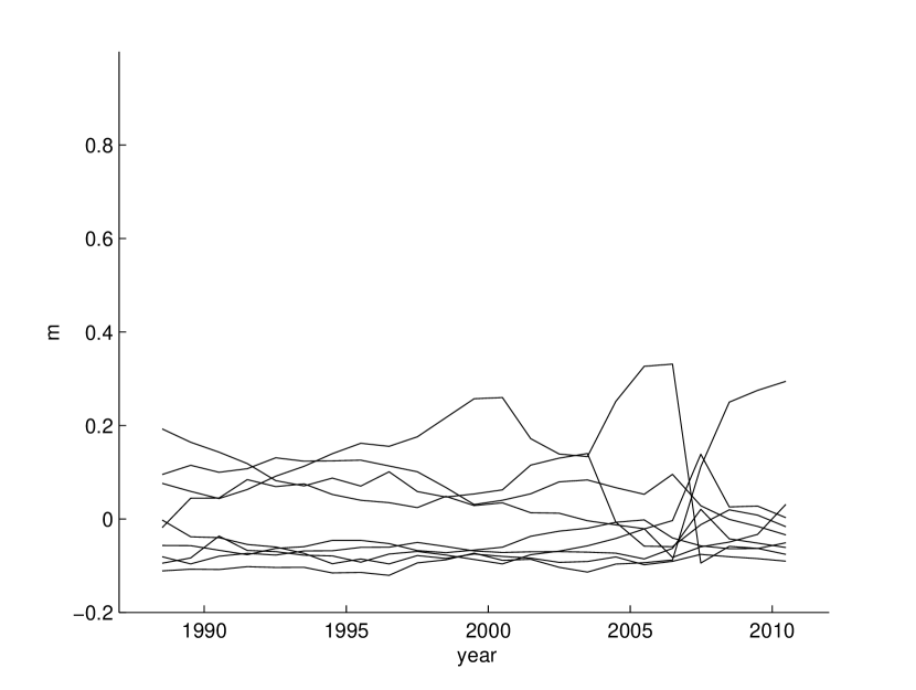
We analyzed the significance of the order parameter by assigning a random value for the sector to each stock. In figure 6 we show one representative result of such a random assignment. Compared with figure 5, the large values of disappear. Before and after 2006 behaves similar as in a disordered phase. The structure observed near 2006 cannot be removed by re-shuffling, because a substantial part of the stocks change their values of . If there would be only one stock in each IT or financial sector responsible for the transition seen in figure 5, one would get the same behavior. The fluctuation size of in the order of indicates the error on the estimation of . This shows that the observed values for the IT and financial sector are far out of the range of random fluctuations.
References
- Ahlgren and Antell (2010) Ahlgren N, Antell J (2010) Stock market linkages and financial contagion: A cobreaking analysis. The Quarterly Review of Economics and Finance 50, 157–166.
- Alfarano et al. (2005) Alfarano S, Lux T, Wagner F (2005) Estimation of agent-based models: The case of an asymmetric herding model. Comp. Economics 26 19-49.
- Adcock et al. (2012) Adcock CJ, Cortez MC, Rocha Armada MJ, Silva F (2012) Time varying betas and the unconditional distribution of asset returns. Quantitative Finance 12(6), 951–967.
- Beile and Candelon (2011) Beine M, Candelon B (2011) Liberalization and stock market co-movement between emerging economies. Quantitative Finance 12(2): 299–312.
- Black et al. (1972) Black F, Jensen MC, Scholes M (1972) The Capital Asset Pricing Model. Some Empirical Tests in Studies in the Theory of Capital Markets. M Jensen ed.:New York, Praeger Publishers.
- Bos and Newbold (1991) Bos T, Newbold P (1984) An Empirical Investigation of the Possibility of Stochastic Systemic Risk in the Market Model. The Journal of Business 57(1.1), 35–41.
- Bodurtha and Mark (1991) Bodurtha JN, Mark NC (1991) Testing the CAPM with Time-Varying Risk and Returns.
- Bollerslev et al. (1988) Bollerslev T, Engle R, Wooldridge J (1988) A Capital Asset Pricing Model with Time-Varying Covariances. Journal of Political Economy 96(1), 116–131.
- Borland and Hassid (2010) Borland L, Hassid Y (2010) Market Panic on different Time-scales. arXiv:010.4917v1.
- Bornholdt (2001) Bornholdt S (2001) Expectation bubbles in a spin model of markets. Int. Journal of Mod. Physics C 12 667-674.
- Brock and Hommes (1998) Brock WA, Hommes, CH (1998) Heterogeneous beliefs and routes to chaos in a simple asset pricing model. Journal of Economic Dynamics and Control 22, 1235–1274.
- Burda et al. (2004) Burda Z, Görlich A, Jarosz A, Jurkiewicz J (2004) Signal and noise in correlation matrix. Physica A 343(2004)295.
- Chiarella et al. (2010) Chiarella C, Dieci R, He X (2010) A framework for CAPM with heterogeneous beliefs. Springer, pp. 353–369. in: Nonlinear Dynamics in Economics, Finance and Social Sciences: Essays in Honour of John Barkley Rosser Jr., Eds. Bischi, G.-I., C. Chiarella and L. Gardini.
- Citeau et al. (2001) Citeau P, Potters M, Bouchaud JP (2001) Correlation structure of extreme stock returns. Quantitative Finance 1, 217–222.
- Cont and Bouchaud (2000) Cont R, Bouchaud JP (2000) Herd behaviour and aggregate fluctuations in financial markets. Macroeconomic Dynamics 4 170.
- Cont (2001) Cont R (2001) Empirical properties of asset returns: stylized facts and statistical issues. Quantitatve Finance 1 223.
- Dichev et al. (2012) Dichev ID, Huang K, Zhou D (2012) The Dark Side of Trading. Emory Law and Economics Research Paper No. 11-95.
- Fama and French (1992) Fama EF, French KR (1992) The Cross-Section of Expected Stock Returns. The Journal of Finance 47(2), 427–465. The Journal of Finance 46(4), 1485–1505.
- Galluccio et al. (1998) Galluccio S, Bouchaud JP, Potters M (1998) Rational decisions, random matrices and spin glasses. Physica A 259:449–456.
- Harvey and Siddique (2000) Harvey CJ, Siddique A (2000) Conditional Skewness in Asset Pricing Tests. The Journal of Finance LV(3), 1263–1295.
- Kenett et al. (2011) Kenett DY, Shapira Y, Madi A, Bransburg-Zabary S, Gur-Gershgoren G, Ben-Jacob E (2011) Index Cohesive Force Analysis Reveals That the US Market Became Prone to Systemic Collapses Since 2002. PLoS ONE 6(4): e19378.
- Kenett et al. (2012a) Kenett DY, Preis T, Gur-Gershgoren G, Ben-Jacob E (2012a) Dependency Network and node influence: Application to the study of financial markets. Int. J. Bifurcation Chaos 22, DOI: 10.1142/S0218127412501817.
- Kenett et al. (2012b) Kenett DY, Raddant M, Lux T, Ben-Jacob E (2012b) Evolvement of Uniformity and Volatility in the Stressed Global Financial Village. PLoS ONE 7(2): e31144.
- Kirman (1993) Kirman A (1993) Ants, rationality and recruitment. Quart. Jour. of Economics 108 137-156.
- Laloux et al. (1999) Laloux L, Cizeau P, Bouchaud JP, Potters M (1999) Noise Dressing of Financial Correlation Matrices. Phys.Rev.Lett.83 1467.
- Lintner (1965) Lintner J (1965) The Valuation of Risk Assets and the Selection of Risky Investments in Stock Portfolios and Capital Budgets. Review of Economics and Statistics 47, 13–37.
- Livan et al. (2011) Livan G, Alfarano S, Scalas E (2011) Fine structure of spectral properties for random correlation matrices, Phys.Rev. E 84 016113.
- Livan et al. (2012) Livan G, Inoue J, Scalas E (2012) On the non-stationarity of financial time series: impact on optimal portfolio selection. JSTAT, doi: 10.1088/1742-5468/2012/07/P07025.
- Lux and Ausloos (2002) Lux T, Ausloos M (2002) Market fluctuations I: scaling, multi-scaling and their possible origins. In: A Bunde, J Kopp and H Schellhuber(eds.) Theory of Desaster, Springer, Berlin, p.373.
- Marĉenko and Pastur (1967) Marĉenko VA, Pastur LA (1967) Distribution of eigenvalues for some sets of random matrices. Math.USSR-Sb 1(1967)457.
- Messiah (1967) Messiah A (1967) Quantum Mechanics Volume I, North Holland.
- Münnix et al. (2012) Münnix MC, Shimada T, Schäfer R, Leyvraz F, Seligman T, Guhr T, Stanley HE (2012) Identifying States of a Financial Market. Scientific Reports 2(644).
- Pearson (1885) Pearson K (1885) Notes on regression and inheritance in the case of two parents, Proceedings of the Royal Society of London 58 240:242.
- Plerou et al. (2002) Plerou V et al. (2002) Random matrix approach to cross correlations in financial data, Physical Review E 65, 066126.
- Preis et al. (2011) Preis T, Schneider JJ, Stanley HE (2011) Switching processes in financial markets. Proceedings of the National Academy of Sciences doi:10.1073/pnas.1019484108.
- Sharpe (1964) Sharpe W (1964) Capital Asset Prices: a Theory of Market Equilibrium Under Conditions of Risk. Journal of Finance 19, 425–442.
- Stauffer and Sornette (1999) Stauffer D, Sornette D (1999) Self-organized percolation model for stock market fluctuation. Physica A 271 496-506.
- Tumminello et al. (2005) Tumminello M, Aste T, Di Matteo T, Mantegna RN (2005) A tool for filtering information in complex systems. Proceedings of the National Academy of Sciences of the United States of America 102(30):10421-10426.
- Wagner (2006) Wagner F (2006) Application of Zhangs square root law and herding to financial markets. Physica A 364 369-384.
- Wishart (1928) Wishart J (1928) The generalized product moment distribution in samples from a normal multivariate population. Biometrica 20A(1928), 32-52.
- Wu (1982) Wu FY (1982) The Potts model. Rev.Mod.Phys.54(1):235–268.