Eigenvalue Spectra of Modular Networks

Abstract

A large variety of dynamical processes that take place on networks can be expressed in terms of the spectral properties of some linear operator which reflects how the dynamical rules depend on the network topology. Often such spectral features are theoretically obtained by considering only local node properties, such as degree distributions. Many networks, however, possess large-scale modular structures that can drastically influence their spectral characteristics, and which are neglected in such simplified descriptions. Here we obtain in a unified fashion the spectrum of a large family of operators, including the adjacency, Laplacian and normalized Laplacian matrices, for networks with generic modular structure, in the limit of large degrees. We focus on the conditions necessary for the merging of the isolated eigenvalues with the continuous band of the spectrum, after which the planted modular structure can no longer be easily detected by spectral methods. This is a crucial transition point which determines when a modular structure is strong enough to affect a given dynamical process. We show that this transition happens in general at different points for the different matrices, and hence the detectability threshold can vary significantly depending on the operator chosen. Equivalently, the sensitivity to the modular structure of the different dynamical processes associated with each matrix will be different, given the same large-scale structure present in the network. Furthermore, we show that, with the exception of the Laplacian matrix, the different transitions coalesce into the same point for the special case where the modules are homogeneous, but separate otherwise.

Networks form the substrate of a dominating class of interacting complex systems, on which various dynamical processes take place. Many of the most important types of dynamics such as random walks Noh and Rieger (2004); Samukhin et al. (2008), diffusion, synchronization Barahona and Pecora (2002); Arenas et al. (2008); Almendral and Díaz-Guilera (2007) and epidemic spreading Wang et al. (2003); Castellano and Pastor-Satorras (2010); Goltsev et al. (2012) have central properties which are directly expressed via the spectral features of matrices associated with the network topology Dorogovtsev et al. (2003); Chung et al. (2003); Kim and Motter (2007), such as the mixing time of random walks, epidemic thresholds and the synchronization speed of oscillators, to name a few. Virtually all of these processes will be affected by large-scale modular structures present in the network Newman (2011), which is reflected in its spectral properties Ergün and Kühn (2009); Kühn and van Mourik (2011); Chauhan et al. (2009); Nadakuditi and Newman (2012). Since such large-scale modularity is a ubiquitous property in real networks Newman (2011), describing the spectral features resulting from this is a crucial step in understanding how these systems function. Additionally, the information encoded in the eigenvectors of these matrices are central to the nontrivial task of detecting large-scale features in empirical networks Fortunato (2010); Newman (2006); Fiedler (1973); Pothen et al. (1990); Nadakuditi and Newman (2012), and from it is possible to derive general bounds on the detectability of existing community structure Nadakuditi and Newman (2012).

In this work, we formulate an unified framework to obtain the eigenvalue spectrum associated with arbitrary modular structures, parameterized as stochastic block models Holland et al. (1983); Fienberg et al. (1985); Faust and Wasserman (1992); Karrer and Newman (2011). The framework allows the straightforward calculation of a large class of matrices which include the adjacency, Laplacian and normalized Laplacian matrices, and is exact in the limit of large degrees. It contrasts with previous work Kühn and van Mourik (2011) which is exact in the limit of small degrees, but depends on the solution of a number of self-consistency equations which are solved stochastically. Here we show that if the block structure is sufficiently well pronounced, it will trigger the appearance of isolated eigenvalues, with associated eigenvectors strongly correlated with the block partition. If the block structure becomes too weak (but nonvanishing), the isolated eigenvalues merge with the continuous band, and the eigenvectors are no longer correlated with the block partition. This has important consequences to the detectability of modular structure in networks Nadakuditi and Newman (2012) but also to a large class of dynamical processes since after this transition takes place one should not expect the modular structure to play a significant role. We show that in general the different matrices have different sensitivities to the imposed block structure, and exhibit these transitions for different modularity strengths.

Unified framework. — Any given undirected network can be encoded via its adjacency matrix $\bm{A}$, which has entries $A_{ij}=1$ if node $i$ is adjacent to $i$, or $A_{ij}=0$ otherwise. The Laplacian matrix is defined as $\bm{L}=\bm{D}-\bm{A}$, where $\bm{D}$ is a diagonal matrix containing the vertex degrees, $D_{ij}=\delta_{ij}k_{i}$. Finally, the normalized Laplacian is defined as $\bm{\mathcal{L}}=\bm{I}-\bm{D}^{-1/2}\bm{A}\bm{D}^{-1/2}$. Here we use a general parametrization which contains these matrices as special cases, via the matrix $\bm{W}=\bm{C}+\bm{M}$, where $\bm{C}$ is a random diagonal matrix, and $\bm{M}$ is a random symmetric matrix. Simply by choosing $\{\bm{C}=0,\bm{M}=\bm{A}\}$, $\{\bm{C}=D,\bm{M}=-\bm{A}\}$ and $\{\bm{C}=\bm{I},\bm{M}=-\bm{D}^{-1/2}\bm{A}\bm{D}^{-1/2}\}$, we recover $\bm{A}$, $\bm{L}$ and $\bm{\mathcal{L}}$, respectively. We may write $\bm{W}=\bm{C}+\bm{\mathcal{M}}+{\left<\bm{M}\right>}=\bm{\mathcal{X}}+{\left<\bm{M}\right>}$, such that the matrix $\bm{\mathcal{X}}=\bm{C}+\bm{\mathcal{M}}$, with $\bm{\mathcal{M}}=\bm{M}-{\left<\bm{M}\right>}$, has off-diagonal entries with zero mean. The spectrum of $\bm{\mathcal{X}}$ can be obtained via its average resolvent ${\left<(z\bm{I}-\bm{\mathcal{X}})^{-1}\right>}$, using the Stieltjes transform $\rho(z)=-\frac{1}{N\pi}\operatorname{Im}\operatorname{Tr}{\left<(z\bf{I}-\bm{\mathcal{X}})^{-1}\right>}$, with $z$ approaching the real line from above. Given an arbitrary random matrix $\bm{X}$ with zero-mean off-diagonal entries, if the variance of the entries is sufficiently large, we can use the approximation Nadakuditi and Newman (2013),

$${\left<[\bm{X}^{-1}]_{ii}\right>}\simeq\sum_{X_{ii}}\frac{P^{i}(X_{ii})}{X_{ii}-\sum_{j}{\left<[\bm{X}^{-1}]_{jj}\right>}{\left<a^{2}_{j}\right>}},$$ (1)

and ${\left<[\bm{X}^{-1}]_{ij}\right>}=0$ for $i\neq j$, where $\bm{a}$ is the $i$th column of $\bm{X}$, with the diagonal element removed, and it is assumed that the diagonal elements $X_{ii}$ can only take discrete values, distributed according to $P^{i}(X_{ii})$. We use Eq. 1 to compute the average resolvent of the matrix $\bm{\mathcal{X}}$. We consider random graphs parameterized as stochastic block models Holland et al. (1983); Fienberg et al. (1985); Faust and Wasserman (1992) where $N$ nodes are divided into $B$ distinct blocks, where each block $r$ has $n_{r}$ nodes, and the matrix entry $e_{rs}$ specifies the number of edges between blocks $r$ and $s$, which are otherwise randomly placed. Hence, in the considered cases, the expected value of $\bm{M}$ is simply a function of the block memberships, i.e. ${\left<C_{ii}\right>}=[\bm{C}_{B}]_{b_{i},b_{i}}=c_{b_{i}}$ and ${\left<M_{ij}\right>}=[\bm{M}_{B}]_{b_{i},b_{j}}$, with $\bm{C}_{B}$ and $\bm{M}_{B}$ being matrices of size $B\times B$, and the vector $\bm{b}$ of size $N$ and entries in the range $[1,B]$ specifies the block memberships. When applying this to Eq. 1 with $\bm{X}=z\bm{I}-\bm{\mathcal{X}}$, we may use the fact the averages on both sides of Eq. 1 can only depend on the block membership of the respective nodes. Thus, using the shorthand $t_{r}(z)\equiv{\left<[(z\bm{I}-\bm{\mathcal{X}})^{-1}]_{ii}\right>}$ for $i\in r$, we obtain,

$$t_{r}(z)=\sum_{c}\frac{p^{r}_{c}}{z-c-\sum_{s}\sigma^{2}_{rs}n_{s}t_{s}(z)},$$ (2)

where $p^{r}_{c}$ is probability distribution of the diagonal elements $c$ for block $r$, and $\sigma^{2}_{rs}$ is the variance of the elements of $\bm{\mathcal{M}}$, labeled according to block membership, which is identical to the variance of $\bm{M}$. The spectrum of $\bm{\mathcal{X}}$ may be finally obtained via

$$\rho(z)=-\frac{1}{N\pi}\sum_{r}n_{r}\operatorname{Im}t_{r}(z).$$ (3)

In order to obtain the spectrum of $\bm{W}$, we employ an argument developed in Ref. Benaych-Georges and Nadakuditi (2011), and note that in order for $z$ to be an eigenvalue of $\bm{W}=\bm{\mathcal{X}}+\bm{M}$, we must have $\det(z\bm{I}-(\bm{\mathcal{X}}+{\left<\bm{M}\right>}))=0$, which can be rewritten as $\det(z\bm{I}-\bm{\mathcal{X}})\det(\bm{I}-(z\bm{I}-\bm{\mathcal{X}})^{-1}{\left<\bm{M}\right>})=0$. Thus, if the second determinant is zero for a given $z$, it will be an eigenvalue of $\bm{W}$ but not of $\bm{\mathcal{X}}$. These additional eigenvalues may be obtained via the ensemble average $\det(\bm{I}-{\left<(z\bm{I}-\bm{\mathcal{X}})^{-1}\right>}{\left<\bm{M}\right>})=0$, which will hold if the matrix ${\left<(z\bm{I}-\bm{\mathcal{X}})^{-1}\right>}{\left<\bm{M}\right>}$ has an eigenvalue equal to one. Since this matrix has a maximum rank equal to $B$, its nonzero eigenvalues will be identical to the $B\times B$ matrix $\bm{T}(z)\bm{M}_{B}\bm{N}$, where $\bm{T}(z)$ and $\bm{N}$ are diagonal $B\times B$ matrices containing the values of $t_{r}(z)$ and $n_{r}$, respectively. Hence, the existence of additional eigenvalues of $\bm{W}$ may obtained by solving,

$$\det(\bm{I}_{B}-\bm{T}(z)\bm{M}_{B}\bm{N})=0,$$ (4)

simultaneously with $\rho(z)=0$. Eqs. 2, 3 and 4 provide a complete recipe for obtaining the desired spectrum, provided we know the $B\times B$ matrices $\sigma^{2}_{rs}$ and $\bm{M}_{B}$ as well as the diagonal entry distribution $p^{r}_{c}$. For the three matrices of interest they are easily computed as $\{p^{r}_{c}=\delta_{0,c};\;\sigma^{2}_{rs}=[\bm{M}_{B}]_{rs}=e_{rs}/n_{r}n_{s}\}$ for $\bm{A}$, $\{p^{r}_{c}=P(c,e_{r}/n_{r});\;[\bm{M}_{B}]_{rs}=-e_{rs}/n_{r}n_{s};\;\sigma^{2}_{rs}=e_{rs}/n_{r}n_{s}\}$ for $\bm{L}$, with $P(c,\lambda)$ being a Poisson distribution on $c$ with average $\lambda$, and $\{p^{r}_{c}=\delta_{1,c};\;[\bm{M}_{B}]_{rs}=-e_{rs}/\sqrt{n_{r}e_{r}n_{s}e_{s}};\;\sigma^{2}_{rs}\simeq e_{rs}/e_{r}e_{s}\}$ for $\bm{\mathcal{L}}$. We emphasize that, since the approximation in Eq. 1 was used, the obtained spectrum should be correct only in the limit of sufficiently large degrees. If this holds, the theory reproduces in very good detail the spectrum of empirical networks, as can be seen in Fig. 1. The spectrum is composed of a continuous band, as well as a number of isolated eigenvalues, which correspond very well to the solutions of Eqs. 3 and 4, respectively. The same is true for the spectrum of the matrices $\bm{\mathcal{L}}$ and $\bm{L}$ (Fig. 2). The spectrum of $\bm{L}$ is special, since it contains an elaborate fine structure, with many fringes, and an interleaving of the continuous band (Eq. 3) with the isolated eigenvalues (Eq. 4). The continuous band has no well-defined edge, with fringes which extend through the whole spectrum, but with decaying amplitudes. Despite such detailed structure, the theory captures these features very well, as can be seen in Fig. 2 (see also the Supplemental Material).

\begin{overpic}[unit=1cm,width=216.81pt,trim=0.0pt 0.0pt 0.0pt 0.0pt,clip]{example_adj_N20000_ak300_nalt25-band.pdf} \put(18.0,32.0){\includegraphics[width=62.87344pt]{example_graph.pdf}} \put(70.0,25.0){\includegraphics[width=62.87344pt]{example_graph_matrix.pdf}} \end{overpic}

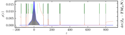
Figure 1: Top: Continuous band of the matrix $\bm{A}$ for the block structure in the inset (right: $e_{rs}$ matrix and block sizes $n_{r}$, left: graphical representation). The solid line corresponds to Eq. 3, and the grey histogram is averaged over $25$ network realizations with $N=2\times 10^{4}$, and ${\left<k\right>}=300$.Bottom: The same, but with the isolated eigenvalues added. The grey vertical lines are average empirical values, whereas the solid (orange) curve corresponds to the determinant of Eq. 4. The vertical (green) line segments mark the eigenvalues of the matrix $\bm{C}_{B}+\bm{M}_{B}\bm{N}$.

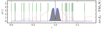
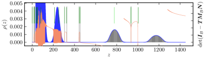
Figure 2: Eigenvalue spectrum of the normalized Laplacian matrix $\bm{\mathcal{L}}$ (top) and Laplacian matrix $\bm{L}$ (bottom) for the block structure of Fig. 1.

For isolated eigenvalues which are sufficiently detached from the spectral band, Eq. 2 may be approximated by $t_{r}\approx 1/(z-c_{r})$, in which case Eq. 4 amounts to $\det(z\bm{I}_{B}-(\bm{C}_{B}+\bm{M}_{B}\bm{N}))=0$, where $\bm{C}_{B}$ is a diagonal matrix with the $c_{r}$ values. If this holds, the detached eigenvalues will correspond to the spectrum of the matrix $\bm{C}_{B}+\bm{M}_{B}\bm{N}$.

At the edges of the continuous band the purely real solution to Eq. 2 becomes unstable, and the largest eigenvalue of the Jacobian $J_{rs}(z)\equiv\partial\hat{t}_{r}/\partial t_{s}=\sum_{c}p^{r}_{c}\sigma^{2}_{rs}n_{s}/(z-c-\sum_{s}\sigma^{2}_{rt}n_{t}t_{t}(z))^{2}$, where $\hat{t}_{r}$ is the right-hand side of Eq. 2, becomes equal to one. Hence, one may find the edges of the continuous band by solving $\det(\bm{I}_{B}-\bm{J}(z))=0$, simultaneously with $\rho(z)=0$.

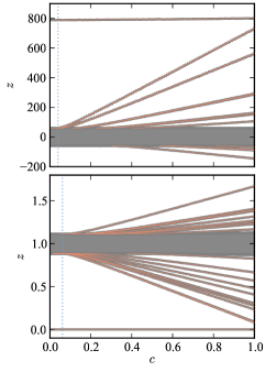
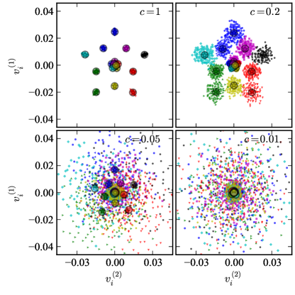
Figure 3: Left: Extremal eigenvalues of $\bm{A}$ (top) and $\bm{\mathcal{L}}$ (bottom), for the block structure of Fig. 1, as a function of the parameter $c$ defined in the text. The solid lines are solutions of Eq. 4, and the data points are empirical values for $N=2\times 10^{4}$. The dotted vertical line marks the detachment transition. Right, top (bottom): Eigenvector values for second and third largest (smallest) eigenvalues of $\bm{A}$ ($\bm{\mathcal{L}}$), for different values of $c$. The circles (stars) correspond to the empirical (theoretical) average values for each block.

Eigenvectors. — The eigenvector equation $(\bm{\mathcal{X}}+\bm{M})\bm{v}=z\bm{v}$ can be rewritten as $(z\bm{I}-\mathcal{X})^{-1}\bm{M}\bm{v}=\bm{v}$. Taking the ensemble average, we get ${\left<(z\bm{I}-\mathcal{X})^{-1}\right>}\bm{M}{\left<\bm{v}\right>}={\left<\bm{v}\right>}$. Since the average values of $\bm{v}$ can only depend on the block memberships, and ${\left<(z\bm{I}-\mathcal{X})^{-1}\right>}$ is diagonal we get

$$\bm{T}(z)\bm{M}_{B}\bm{N}\bm{v}_{B}=\bm{v}_{B},$$ (5)

where $\bm{v}_{B}$ contain the average values of $v$ for each block.

If the block structure is made sufficiently tenuous, all but the most extremal detached eigenvalues will approach progressively the continuous band. At some point, before the graph becomes fully random, they will merge with the continuous band, and the associated eigenvectors will no longer convey any information on the existing block structure. An example is shown in Fig. 3, which shows the full spectrum of the block structure given by $e_{rs}=ce_{rs}^{0}+(1-c)e^{0}_{r}e^{0}_{s}/2E$, with $e_{rs}^{0}$ being the same block structure shown in Fig. 1, and $e^{0}_{r}=\sum_{s}e_{rs}^{0}$. The parameter $c$ interpolates between a random graph ($c=0$) and the original block structure ($c=1$), while preserving the same degree distribution. As show in Fig. 3, for a specific value of $c=c^{*}>0$ all but the most extremal eigenvalue merge with the continuous band, and for $c<c^{*}$ the eigenvector values are no longer discernibly correlated with the planted block structure. It is important to notice that the transition point $c^{*}$ is different for the matrices $\bm{A}$ and $\bm{\mathcal{L}}$, and thus the different spectra will have different sensitivities to the planted block structure. This can be seen in more detail by considering a simpler two-block system with $n_{1}/N=w$, $n_{2}/N=1-w$ and $e_{rs}=E[c\delta_{rs}+(1-c)/2]$, which is a diagonal block structure with the parameter $c$ controlling the block segregation and $w$ the degree asymmetry . In Fig. 4 is shown the extremal eigenvalues for the three matrices as a function of $c$, compared with empirical values. For the normalized Laplacian matrix $\bm{\mathcal{L}}$, the extremal eigenvalue is very insensitive to the parameter $w$ . The matrix $\bm{A}$ displays, on the other hand, different transition points, depending on $w$, with larger values of $c^{*}$ for larger degree asymmetries. The spectral band for the matrix $\bm{L}$ has no well-defined edge; hence, the transition point on a finite network will depend on the system size. The observable edge of the band is obtained by computing the extremal statistics of $\rho(z)$ (see the Supplemental Material), and matches well the observed values, as can be seen in Fig. 4. A comparison of the transition points can be seen in the lower right of Fig. 4, where it is also included the values for the modularity matrix $\bm{B}=\bm{A}-\bm{k}\bm{k}^{T}/2E$, where $\bm{k}$ is a vector with node degrees, often used for community detection Newman (2006), which can also be calculated with the presented method in an entirely analogous fashion. Since for this specific block structure it has systematically the lowest threshold $c^{*}$ among the others, this seems to corroborate the hypothesis in Refs. Nadakuditi and Newman (2012); Radicchi (2013) that $\bm{B}$ may posses optimal characteristics in some scenarios. On the other hand, the comparatively worst behavior of the Laplacian $\bm{L}$ raises issues with its use for this purpose (as in e.g. Ref. Newman (2013)).

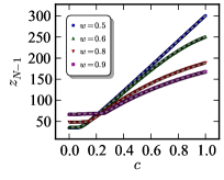
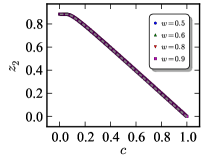
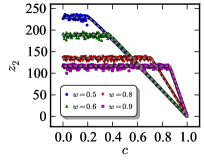
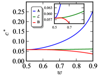
Figure 4: Top, left (right): Second largest (smallest) eigenvalue of $\bm{A}$ ($\bm{\mathcal{L}}$), for the asymmetric two-block structure described in the text. The dashed curves are the theoretical values, and the data points are obtained from network realizations with $N=2\times 10^{4}$ and ${\left<k\right>}=300$. Bottom, left: Second smallest eigenvalue of $L$. The dashed curves are the expected values for $N=2\times 10^{4}$ (see Supplemental Material). Bottom, right: Transition point $c^{*}$ as a function of $w$ for the matrices $\bm{A}$, $\bm{\mathcal{L}}$ and the modularity matrix $\bm{B}$.

Homogeneous blocks.— Further analytical progress can be made by assuming that the blocks are homogeneous, such that the right-hand side of Eq. 2 is the same for all blocks. This means that they must all share the same properties such as size $n_{r}$ and average degree $e_{r}/n_{r}$. The solution in case $p^{r}_{c}=\delta_{d,c_{r}}$ (i.e. for both $\bm{A}$ and $\bm{\mathcal{L}}$) will then be simply $t(z)=(z-d\pm\sqrt{(d-z)^{2}-4a})/2a$ with $a=a_{r}=N\sum_{s}\sigma_{rs}^{2}/B$, which will result in the usual semicircle distribution $\rho(z)=\sqrt{4a-(z-d)^{2}}/2a\pi$ for $|z-d|<2\sqrt{a}$; otherwise, $\rho(z)=0$. The detached eigenvalues will be given by the solution of $\det(\bm{I}-t(z)N\bm{M}_{B}/B)=0$. Hence there will be a one-to-one correspondence between the nonzero eigenvalues $\lambda_{i}$ of $\bm{M}_{B}$ and the detached eigenvalues $z_{i}=d+at_{i}+1/t_{i}$, where $t_{i}=B/N\lambda_{i}$, as long as $|z_{i}-d|>2\sqrt{a}$; otherwise, they will merge with the continuous band. By making $|z_{i}-d|=2\sqrt{a}$, one obtains that this transition happens at $\lambda_{i}=\pm\sqrt{a}B/N$. Both for $\bm{A}$ and $\bm{\mathcal{L}}$ one can see that this transition occurs at the same point: If one writes the block matrix as $e_{rs}=N{\left<k\right>}m_{rs}$, such that $\sum_{rs}m_{rs}=1$, this transition translates to

$$\lambda_{m}^{2}=\frac{1}{{\left<k\right>}B^{2}},$$ (6)

where $\lambda_{m}$ is an eigenvalue of the $m_{rs}$ matrix. The fact that the detachment transition is identical for both $\bm{A}$ and $\bm{\mathcal{L}}$ is a special property of the homogeneous block structure, and does not hold in general, as we have shown previously .

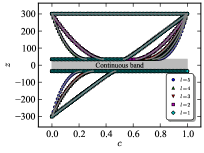
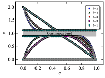
$l=1$

$l=2$

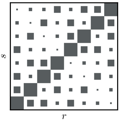
$l=3$

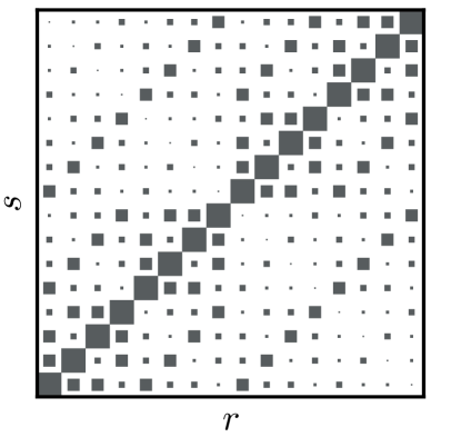
$l=4$

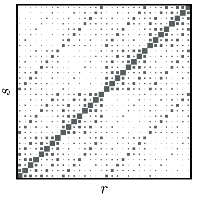
$l=5$

Figure 5: Top: Detachment transitions for the nested partition model described in the text with $B_{1}=2$ as a function of the mixing parameter $c$, and for different nesting depths $l$, for $\bm{A}$ and $\bm{\mathcal{L}}$. The data points correspond to network realizations with $N=2\times 10^{4}$ and ${\left<k\right>}=300$, and the solid lines are theoretical values. Bottom: Example of $e_{rs}$ matrices with $B_{1}=2$ for different values of $l$.

As a concrete example of an homogeneous structure, we consider a nested version of the usual planted partition model Condon and Karp (2001), inspired by similar constructions done in Refs. Leskovec et al. (2008); Palla et al. (2010). We define a seed structure with $B_{1}$ blocks and $[\bm{m}_{1}]_{rs}=\delta_{rs}c/B_{1}+(1-\delta_{rs})(1-c)/B_{1}(B_{1}-1)$, and construct a nested matrix of depth $l$ via $\bm{m}_{l}=\bm{m}_{l-1}\otimes\bm{m}_{l-1}$ where $\otimes$ denotes the Kronecker product. The eigenvalues of the matrix $\bm{m}_{l}$ are given by $\lambda^{i}_{m_{l}}=((cB_{1}-1)/(B_{1}(B_{1}-1)))^{l-i}/{B_{1}^{i}}$, for $i\in[0,l]$. Thus, from Eq. 6 one obtains a series of transitions, where a deeper level of the nested structure “fades away,” and the spectrum is indistinguishable from that of a $l-1$ structure (see Fig. 5). The transition of the shallowest level happens at ${\left<k\right>}=((B-1)/(cB-1))^{2}$, which is the same as the regular planted partition model Nadakuditi and Newman (2012). This transition marks the point at which more general inference methods should also fail to detect the imposed partition Decelle et al. (2011).

In summary, we presented an unified framework to obtain the full spectrum of random networks with modular structure, in the limit of large degrees. We showed that the detachment transition of the isolated eigenvalues is a general feature which determines how strongly the existing modular structure affects the different spectra. The different matrices react differently to the imposed modular structure and have different transition points. Only when the blocks are homogeneous do some of these transitions collapse together. Hence, in general, the detectability threshold of the imposed block structure may depend strongly on the actual spectrum which is observed.

See pages - of sup_mat.pdf

References

- Noh and Rieger (2004) J. D. Noh and H. Rieger, Physical Review Letters 92, 118701 (2004).
- Samukhin et al. (2008) A. N. Samukhin, S. N. Dorogovtsev, and J. F. F. Mendes, Physical Review E 77, 036115 (2008).
- Barahona and Pecora (2002) M. Barahona and L. M. Pecora, Physical Review Letters 89, 054101 (2002).
- Arenas et al. (2008) A. Arenas, A. Díaz-Guilera, J. Kurths, Y. Moreno, and C. Zhou, Physics Reports 469, 93 (2008).
- Almendral and Díaz-Guilera (2007) J. A. Almendral and A. Díaz-Guilera, New Journal of Physics 9, 187 (2007).
- Wang et al. (2003) Y. Wang, D. Chakrabarti, C. Wang, and C. Faloutsos, in 22nd International Symposium on Reliable Distributed Systems, 2003. Proceedings (2003) pp. 25–34.
- Castellano and Pastor-Satorras (2010) C. Castellano and R. Pastor-Satorras, Physical Review Letters 105, 218701 (2010).
- Goltsev et al. (2012) A. V. Goltsev, S. N. Dorogovtsev, J. G. Oliveira, and J. F. F. Mendes, Physical Review Letters 109, 128702 (2012).
- Dorogovtsev et al. (2003) S. N. Dorogovtsev, A. V. Goltsev, J. F. F. Mendes, and A. N. Samukhin, Physical Review E 68, 046109 (2003).
- Chung et al. (2003) F. Chung, L. Lu, and V. Vu, Proceedings of the National Academy of Sciences 100, 6313 (2003).
- Kim and Motter (2007) D.-H. Kim and A. E. Motter, Physical Review Letters 98, 248701 (2007).
- Newman (2011) M. E. J. Newman, Nat Phys 8, 25 (2011).
- Ergün and Kühn (2009) G. Ergün and R. Kühn, Journal of Physics A: Mathematical and Theoretical 42, 395001 (2009).
- Kühn and van Mourik (2011) R. Kühn and J. van Mourik, Journal of Physics A: Mathematical and Theoretical 44, 165205 (2011).
- Chauhan et al. (2009) S. Chauhan, M. Girvan, and E. Ott, Physical Review E 80, 056114 (2009).
- Nadakuditi and Newman (2012) R. R. Nadakuditi and M. E. J. Newman, Physical Review Letters 108, 188701 (2012).
- Fortunato (2010) S. Fortunato, Physics Reports 486, 75 (2010).
- Newman (2006) M. E. J. Newman, Physical Review E 74, 036104 (2006).
- Fiedler (1973) M. Fiedler, Czechoslovak Mathematical Journal 23, 298–305 (1973).
- Pothen et al. (1990) A. Pothen, H. D. Simon, and K.-P. Liou, SIAM Journal on Matrix Analysis and Applications 11, 430 (1990).
- Holland et al. (1983) P. W. Holland, K. B. Laskey, and S. Leinhardt, Social Networks 5, 109 (1983).
- Fienberg et al. (1985) S. E. Fienberg, M. M. Meyer, and S. S. Wasserman, Journal of the American Statistical Association 80, 51 (1985).
- Faust and Wasserman (1992) K. Faust and S. Wasserman, Social Networks 14, 5 (1992).
- Karrer and Newman (2011) B. Karrer and M. E. J. Newman, Physical Review E 83, 016107 (2011).
- Nadakuditi and Newman (2013) R. R. Nadakuditi and M. E. J. Newman, Physical Review E 87, 012803 (2013).
- Benaych-Georges and Nadakuditi (2011) F. Benaych-Georges and R. R. Nadakuditi, Advances in Mathematics 227, 494 (2011).
- Note (1) Note that the parameter does not change the degree distribution.
- Note (2) The curves do change, however only very subtly.
- Radicchi (2013) F. Radicchi, Physical Review E 88, 010801 (2013).
- Newman (2013) M. E. J. Newman, EPL (Europhysics Letters) 103, 28003 (2013).
- Note (3) It can also be shown that Eq. 6 also holds for the modularity matrix .
- Condon and Karp (2001) A. Condon and R. M. Karp, Random Structures & Algorithms 18, 116–140 (2001).
- Leskovec et al. (2008) J. Leskovec, D. Chakrabarti, J. Kleinberg, C. Faloutsos, and Z. Ghahramani, arXiv:0812.4905 (2008).
- Palla et al. (2010) G. Palla, L. Lovász, and T. Vicsek, Proceedings of the National Academy of Sciences 107, 7640 (2010).
- Decelle et al. (2011) A. Decelle, F. Krzakala, C. Moore, and L. Zdeborová, Physical Review Letters 107, 065701 (2011).