Simulation of forward-reverse stochastic representations for conditional diffusions

Abstract

In this paper we derive stochastic representations for the finite dimensional distributions of a multidimensional diffusion on a fixed time interval, conditioned on the terminal state. The conditioning can be with respect to a fixed point or more generally with respect to some subset. The representations rely on a reverse process connected with the given (forward) diffusion as introduced in Milstein, Schoenmakers and Spokoiny [Bernoulli 10 (2004) 281–312] in the context of a forward-reverse transition density estimator. The corresponding Monte Carlo estimators have essentially root-$N$ accuracy, and hence they do not suffer from the curse of dimensionality. We provide a detailed convergence analysis and give a numerical example involving the realized variance in a stochastic volatility asset model conditioned on a fixed terminal value of the asset.

and t2Supported in part by the DFG Research Center Matheon “Mathematics for Key Technologies” in Berlin.

1 Introduction

The central result in this paper is the development of a new generic procedure for simulation of conditioned diffusions, also called diffusion bridges or pinned diffusions. More specifically, for some given (unconditional) diffusion process $X$, we aim to simulate the functional

$$\mathbb{E}\bigl{[}g\bigl{(}X(s_{1}),\ldots,X(s_{R})\bigr{)}|X(T)\in A,X(0)=x\bigr{]},$$ (1)

where $0\leq s_{1}<s_{2}<\cdots<s_{R}<T$, $A$ is some set that may consist of only one point, $g$ is an arbitrarily given suitable test function and $x\in\mathbb{R}^{d}$ is a given state. In recent years, the problem of computing terms such as (1) has attracted a lot of attention in the literature, sparked by several applications. Indeed, many relevant properties of a diffusion process $X$ can be advantageously analyzed by considering the process conditioned on certain appropriate events. One so allows “to study rare events by conditioning on the event happening or to analyze the behaviour of a composite system when only some of its components can be observed,” as is eloquently put by Hairer, Stuart and Voss (2009). For instance, in statistical inference based on a continuous time model, discrete time observations can be enriched to continuous time observations by sampling from the diffusion bridges between the discrete time data; see Lin, Chen and Mykland (2010) and Bladt and Sørensen (2012) for more information. Conditional diffusions have further been successfully used for critical calculations in rare event situations. As an example from computational chemistry, we refer to the review paper of Bolhuis et al. (2002), where diffusion bridges are used for detection of the transition state surface between two stable regions $A$ and $B$ in configuration space. Here, standard Monte Carlo simulation is prohibitively costly, as the event of such a transition is rare, provided that the “walls” in the energy surface between $A$ and $B$ are high. However, by studying the process conditioned on starting in $A$ and ending in $B$, one can efficiently observe on which paths the configuration typically travels from $A$ to $B$. Other possible applications appear in the field of stochastic environmental models, for instance, regarding the concentration evolutions of pollution in water; for example see Spivakovskaya, Heemink and Schoenmakers (2007) and references therein for a related problem.

Several approaches for simulation of diffusion bridges have already been studied in the literature. For the theory of diffusion bridges we refer to Lyons and Zheng (1990) and the references therein. Many existing approaches utilize known Radon–Nikodym densities of the law of the diffusion $X$ conditioned on initial and terminal values, with respect to the law of a standard diffusion bridge process (e.g., Wiener bridge) on path-space [as a Radon–Nikodym derivative obtained by Doob’s h-transform; see, e.g., Rogers and Williams (2000) or Lyons and Zheng (1990)]. Several other approaches are based on (partial) knowledge of the transition densities of the unconditional diffusion (that is not generically available, of course). For an overview of many different techniques, we refer to Lin, Chen and Mykland (2010).

First, let us mention the work by Beskos, Papaspiliopoulos and Roberts (2006) who construct a general, rejection-based algorithm for solutions of one-dimensional SDEs, based on the Radon–Nikodym derivative of the law of the solution with respect to the Wiener measure. The algorithm gives (in finite, but random time) discrete samples of the exact solution of the SDE. A simple adaption of this algorithm gives samples of the exact diffusion process conditioned on $X(T)=y$, by using the law of the corresponding Brownian bridge as reference measure (instead of the Wiener measure). An overview of related importance sampling techniques is given by Papaspiliopoulos and Roberts (2012). On the other hand, by relying on knowledge of the transition densities of $X$, Lin, Chen and Mykland (2010) use a sequential weighted Monte Carlo framework, including resampling with optimal priority scores.

Another general technique used for simulation of diffusion bridges is the Markov chain Monte Carlo method. Indeed, Stuart, Voss and Wiberg (2004) and Hairer, Stuart and Voss (2009) show how the law of a (multi-dimensional, uniformly elliptic, additive-noise) diffusion $X$ conditioned on $X(T)=y$ can be regarded as the invariant distribution of a stochastic differential equation of Langevin type on path-space, that is, of a Langevin-type stochastic partial differential equation (SPDE). Thus, in principle MCMC methods are applicable as explored by Stuart, Voss and Wiberg (2004) and Beskos et al. (2008). However, this requires the numerical solution of the SPDE involved. It should be noted that in Hairer, Stuart and Voss (2011) the uniform ellipticity condition is relaxed leading to a fourth order parabolic SPDE rather than a second order one.

Other notable approaches include those of Milstein and Tretyakov (2004), which treat the case of physically relevant functionals of Wiener integrals with respect to Brownian bridges, and Stinis (2011), who uses an MCMC approach based on successive modifications of the drift of the diffusion process.

Another approach is the one of Bladt and Sørensen (2012) developed for one-dimensional diffusions. In order to obtain a sample from the process $X$ conditioned on $X(0)=x$ and $X(T)=y$, Bladt and Sørensen (2012) start a path of the diffusion from $(0,x)$ and another path of the diffusion in reversed time at $(T,y)$. If these paths hit at time $\tau$, consider the concatenated path $Z$. The distribution of the process $Z$ (conditional on $0\leq\tau\leq T$) equals the distribution of the bridge conditional on being hit by an independent path of the underlying diffusion with initial distribution $p(0,y,T,\cdot)$. As proved by Bladt and Sørensen (2012), the probability of this event approaches $1$ when $T\to\infty$. Finally, in order to improve the accuracy, $Z$ is used as initial value of an MCMC algorithm on path space, converging to a sample from the true diffusion bridge.

A more general approach is given by Delyon and Hu (2006) which relies on the explicit Radon–Nikodym derivative of the diffusion $X$ conditioned on its initial and terminal values and another diffusion $Y$, which is modeled like the Brownian bridge. In fact, $Y$ has the same dynamics as $X$, except for an extra term $-\frac{Y(t)-y}{T-t}$ in the drift, which enforces $Y(T)=y$. Under certain regularity conditions—in particular invertibility of the diffusion matrix $\sigma=\sigma(t,x)$—Delyon and Hu (2006) provide a Girsanov-type theorem, which leads to a representation of the form

$$\mathbb{E}\bigl{[}g(X)|X(0)=x,X(T)=y\bigr{]}=\mathbb{E}\bigl{[}g(Y)Z(Y)\bigr{]}$$

for functionals $g$ defined on path-space and a factor $Z(Y)$ explicitly given as a functional of the path $Y$ together with quadratic variations of functions of $Y$. As such this approach allows for direct Monte Carlo simulation of (1). However, we stress that $Z(Y)$ explicitly depends on $\sigma^{-1}$ which does not exist in many hypo-elliptic applications. On the other hand, simulation of the bridge-type process $Y$ is numerically troublesome because of the exploding drift term.

The new method presented in this article is inspired by the forward-reverse estimator for the transition density $p(0,x,T,y)$ constructed by Milstein, Schoenmakers and Spokoiny (2004). Given a grid $0\leq s_{0}<s_{1}<\cdots<s_{K}=t^{\ast}<t_{1}<\cdots<t_{L}=T$, we prove that

$$\mathbb{E}\bigl{[}g\bigl{(}X(s_{1}),\ldots,X(s_{K}),X(t_{1}),\ldots,X(t_{L-1})\bigr{)}|X(s_{0})=x,X(T)=y\bigr{]}$$

equals

$$\lim_{\varepsilon\to 0}\frac{\mathbb{E}[g(X(s_{1}),\ldots,X(s_{K}),Y(\widehat{t}_{L-1}),\ldots,Y(\widehat{t}_{1}))K_{\varepsilon}(Y(\widehat{t}_{L})-X(t^{\ast}))\mathcal{Y}(\widehat{t}_{L})]}{\mathbb{E}[K_{\varepsilon}(Y(\widehat{t}_{L})-X(t^{\ast}))\mathcal{Y}(\widehat{t}_{L})]},$$ (2)

which can be implemented by Monte Carlo simulation for any $\varepsilon>0$. In (2) $s_{0}<t^{\ast}<T$ is a given grid-point chosen by the user. The process $X$ solves the original SDE with initial value $X(s_{0})=x$ on the time-interval $[s_{0},t^{\ast}]$. On the other hand, $Y$ is an (independent) reverse process as defined in Section 3 started at $Y(0)=y$ and simulated until time $\widehat{t}_{L}:=T-t^{\ast}$, not on the original grid, but on a “perturbed” grid defined in (15). [Note that $Y$ is different from the time-reversed diffusion in the sense of Haussmann and Pardoux (1986) that explicitly requires the transition density of $X$.] Indeed, the dynamics of $Y$ are explicitly given below in terms of the dynamics of $X$—not relying on the transition density—and, usually, share the same regularity properties; see (5) and (2). Next, we weight the trajectories according to the distance between $X(t^{\ast})$ and $Y(T)$ using a kernel $K$ with bandwidth $\varepsilon$. Finally, we have an exponential weighting factor $\mathcal{Y}$, similar to the Radon–Nikodym derivative in Delyon and Hu (2006). The denominator in (2) actually corresponds to the forward-reverse estimator for the transition density $p(s_{0},x,T,y)$ of $X$ introduced by Milstein, Schoenmakers and Spokoiny (2004). The details of the Monte Carlo simulation are spelled out in Section 4, but we note that (2) can be computed to an accuracy of $\varepsilon$ with a complexity of $\mathcal{O}(\varepsilon^{-2})$ in any dimension less or equal to four (disregarding possible discretization errors due to the construction of samples $X$, $Y$ and $\mathcal{Y}$). Thus our algorithm essentially achieves the optimal rate of convergence for Monte Carlo algorithms.

We underline that the forward-reverse algorithm for (1) presented here is not a straightforward extension of the forward-reverse algorithm for transition densities of Milstein, Schoenmakers and Spokoiny (2004). The main difficulty lies in the extension of the representation from just one intermediate time $0<t^{\ast}<T$ to an arbitrary time grid $0\leq s_{0}<s_{1}<\cdots<s_{K}=t^{\ast}<t_{1}<\cdots<t_{L}=T$ with $L>1$. In the nonautonomous case this issue is further complicated due to the fact that the dynamics of the reverse process as defined in Milstein, Schoenmakers and Spokoiny (2004) depends explicitly on both $t^{\ast}$ and $T$. Obviously, the different structure also requires a different error analysis. In particular, we need sharper error bounds than Milstein, Schoenmakers and Spokoiny (2004).

In comparison to the other methods mentioned above, our new procedure has the following main features:

[(iii)]

The method applies to multidimensional diffusions.

It is based on simulation of unconditional diffusions only, hence technical simulation problems due to exploding drifts in SDEs that govern particular diffusion bridges are avoided.

The vector fields determining the (forward) SDE that governs $X$ only need to satisfy a Hörmander-type condition guaranteeing sufficient regularity and exponential decay of the transition densities. In particular, the diffusion matrix of $X$ may be degenerate.

The estimator corresponding to the developed stochastic representation for (1) is root-$N$ consistent, that is the mean square estimation accuracy is of order $\mathcal{O}(N^{-1/2})$ with $N$ being the number of trajectories that need to be simulated.

As a matter of fact, the methods for simulating diffusion bridges known in the literature so far, do not cover all the features (i)–(iv) simultaneously. For example, Delyon and Hu (2006) require that either the diffusion matrix is invertible, or impose some very specific structural conditions on the drift and diffusion matrix of the process $X$. Moreover, the exploding drift terms in their process $Y$ makes simulation of the auxiliary process $Y$ nontrivial. On the other hand, the method of Bladt and Sørensen (2012) in germ carries some ideas related to our approach, but they need to impose balance restrictions on the transition density of $X$, and moreover their method—together with several others—is only one dimensional. The methods of Stuart, Voss and Wiberg (2004) and the related papers mentioned above also involve some further structural assumptions and, in addition, require numerical solutions of SPDEs.

Moreover, we complement our algorithm by an adaptation, which allows us to treat the more general problem of conditioning at final time $T$ not on all, but just on some components of the vector $X_{T}$. More precisely, we present a variant of the algorithm for computing conditional expectations where $X_{T}$ is conditioned to lie in a “simple” set $A$, that is, either $A$ has positive measure both under the Lebesgue measure and the distribution of $X_{T}$, or $A$ is an affine plane of dimension $0\leq d^{\prime}\leq d$. In order to achieve this extension, we need to prove (Lebesgue) integrable error bounds for the forward-reverse algorithm for the case where $X_{T}$ is conditioned to a value $y$.

The structure of the paper is as follows. In Section 2 we recap the essential facts concerning the reverse diffusion system of Milstein, Schoenmakers and Spokoiny (2004). The main representation theorems for the diffusion conditioned on reaching a fixed state, or conditioned on reaching some Borel set, are derived in Section 3. A detailed accuracy analysis concerning the Monte Carlo estimators for the respective conditioned diffusions is provided in Section 4, including the precise required regularity assumptions given in Conditions 4.1, 4.4 and 4.5. Limitations of the method are discussed in Section 4.3, while Section 5 provides a numerical study involving a Heston-type stochastic volatility model.

2 Recap of forward-reverse representations for diffusions

In this section we recapitulate shortly the main ingredients in the approach by Milstein, Schoenmakers and Spokoiny (2004). Let us consider the SDE

$$dX_{t,x}(s)=a\bigl{(}s,X_{t,x}(s)\bigr{)}\,ds+\sigma\bigl{(}s,X_{t,x}(s)\bigr{)}\,dW(s),$$

(3)

$$\eqntext{0\leq s\leq T,X_{t,x}(t)=x,}$$ (4)

where $X_{t,x}\in\mathbb{R}^{d}$, $a\dvtx[t,T]\times\mathbb{R}^{d}\rightarrow\mathbb{R}^{d}$, $\sigma\dvtx[t,T]\times\mathbb{R}^{d}\rightarrow\mathbb{R}^{d\times m}$, $W$ is an $m$-dimensional standard Wiener process and $x\in\mathbb{R}^{d}$. At this stage, we only assume that $X$ admits a $C^{2}$ transition density $p$ and that the coefficients of (2) are $C^{2}$ as well.

Along with the (forward) process $X$ given by (2), Milstein, Schoenmakers and Spokoiny (2004) introduced an associated process $(Y_{t,y;T}(s),\mathcal{Y}_{t,y;T}(s))$ in $\mathbb{R}^{d}\times\mathbb{R}$, $t\leq s\leq T$, termed reverse process on the interval $[t,T]$, that solves the SDE

$$dY_{t,y;T}(s) = \alpha_{t,T}\bigl{(}s,Y_{t,y;T}(s)\bigr{)}\,ds$$ (5)

$${}+\widetilde{\sigma}_{t,T}\bigl{(}s,Y_{t,y;T}(s)\bigr{)}\,d\widetilde{W}(s),\qquad Y_{t,y;T}(t)=y,$$

$$\mathcal{Y}_{t,y;T}(s) = \exp\biggl{(}\int_{t}^{s}c_{t,T}\bigl{(}u,Y_{t,y;T}(u)\bigr{)}\,du\biggr{)}$$

with $\widetilde{W}$ being a (from $W$ independent) $m$-dimensional Wiener process, and

$$\alpha_{t,T}^{i}(s,y) := \sum_{j=1}^{d}\frac{\partial}{\partial y^{j}}b^{ij}(T+t-s,y)-a^{i}(T+t-s,y),\qquad b:=\sigma\sigma^{\top},$$

$$\widetilde{\sigma}_{t,T}(s,y) := \sigma(T+t-s,y),$$ (6)

$$\qquad c_{t,T}(s,y) := \frac{1}{2}\sum_{i,j=1}^{d}\frac{\partial^{2}b^{ij}}{\partial y^{i}\partial y^{j}}(T+t-s,y)-\sum_{i=1}^{d}\frac{\partial a^{i}}{\partial y^{i}}(T+t-s,y).$$

Despite its name, we stress that $(Y,\mathcal{Y})$ is the solution of an ordinary SDE forward in time on the interval $[t,T]$.

One of the central results in Milstein, Schoenmakers and Spokoiny (2004) is the following theorem.

Theorem 2.1 ([M.S.S. (2004)])

For fixed $t,x,y$ and $t<t^{\ast}<T$, and any bi-variate test function $f$we have

$$\mathbb{E}\bigl{[}f\bigl{(}X_{t,x}\bigl{(}t^{\ast}\bigr{)},Y_{t^{\ast},y;T}(T)\bigr{)}\mathcal{Y}_{t^{\ast},y;T}(T)\bigr{]}$$

(7)

$$\qquad=\int\!\!\!\int p\bigl{(}t,x,t^{\ast},x^{\prime}\bigr{)}p\bigl{(}t^{\ast},y^{\prime},T,y\bigr{)}f\bigl{(}x^{\prime},y^{\prime}\bigr{)}\,dx^{\prime}\,dy^{\prime},$$

where $X_{t,x}(s)$ satisfies the forward equation (2), and $(Y_{t^{\ast},y;T}(s),\mathcal{Y}_{t^{\ast},y;T}(s))$, $s\geq t^{\ast}$, is the solution of the reverse system (5).

Corollary 2.2

By taking $f\equiv 1$, (2.1) yields

$$\mathbb{E}\bigl{[}\mathcal{Y}_{t^{\ast},y;T}(T)\bigr{]}=\int p\bigl{(}t^{\ast},y^{\prime},T,y\bigr{)}\,dy^{\prime},$$ (8)

which obviously extends to $t^{\ast}=t$. By next taking $f(x^{\prime},y^{\prime})=f(x^{\prime})$ (while abusing notation slightly) we obtain from (2.1), using (8) and the independence of $X$ and $(Y,\mathcal{Y})$,

$$\mathbb{E}\bigl{[}f\bigl{(}X_{t,x}\bigl{(}t^{\ast}\bigr{)}\bigr{)}\bigr{]}=\int p\bigl{(}t,x,t^{\ast},x^{\prime}\bigr{)}f\bigl{(}x^{\prime}\bigr{)}\,dx^{\prime},$$

which obviously extends to $t^{\ast}=T$, that is, the standard forward stochastic representation for $\int p(t,x,T,x^{\prime})f(x^{\prime})\,dx^{\prime}$. On the other hand, by taking $f(x^{\prime},y^{\prime})=f(y^{\prime})$ we obtain the so called reverse stochastic representation

$$\mathbb{E}\bigl{[}f\bigl{(}Y_{t^{\ast},y;T}(T)\bigr{)}\mathcal{Y}_{t^{\ast},y;T}(T)\bigr{]}=\int p\bigl{(}t^{\ast},y^{\prime},T,y\bigr{)}f\bigl{(}y^{\prime}\bigr{)}\,dy^{\prime},$$ (9)

which obviously extends to $t^{\ast}=t$.

3 Forward-reverse representations for conditional diffusions

It should be noted that in Milstein, Schoenmakers and Spokoiny (2004) the time domain of the reverse process was considered fixed. For our purposes however, it turns out to be more effective (in particular regarding the proof of Theorem 3.2 below) to consider reverse processes suitably defined on different time domains. In particular it turns out be fruitful to formulate the forward-reverse representations of the previous section in terms of reverse processes defined on $[0,T]$ for suitable $T>0$. We therefore introduce the reverseprocess

$$\bigl{(}Y_{y;T}(s),\mathcal{Y}_{y;T}(s)\bigr{)}_{0\leq s\leq T}:=\bigl{(}Y_{0,y;T}(s),\mathcal{Y}_{0,y;T}(s)\bigr{)}_{0\leq s\leq T}$$ (10)

that starts at time $s=0$ at a generic state $(y,1)$, is defined on an interval $[0,T]$ and satisfies (5) with coefficients (2) for $t=0$, that is, (10) solves the SDE

$$dY(s) = \alpha_{0,T}\bigl{(}s,Y(s)\bigr{)}\,ds+\widetilde{\sigma}_{0,T}\bigl{(}s,Y(s)\bigr{)}\,d\widetilde{W}(s),\qquad Y(0)=y,$$

$$\mathcal{Y}(s) = \exp\biggl{(}\int_{0}^{s}c_{0,T}\bigl{(}u,Y(u)\bigr{)}\,du\biggr{)}.$$

As a result, we have for any fixed $t$, $0\leq t\leq T$, that

$$\bigl{(}Y_{y;T}(s),\mathcal{Y}_{y;T}(s)\bigr{)}_{0\leq s\leq T-t}=\bigl{(}Y_{t,y;T}(t+s),\mathcal{Y}_{t,y;T}(t+s)\bigr{)}_{0\leq s\leq T-t},$$

whence (2.1) and (9) may be equivalently written as

$$\mathbb{E}\bigl{[}f\bigl{(}X_{t,x}\bigl{(}t^{\ast}\bigr{)},Y_{y;T}\bigl{(}T-t^{\ast}\bigr{)}\bigr{)}\mathcal{Y}_{y;T}\bigl{(}T-t^{\ast}\bigr{)}\bigr{]}$$

(12)

$$\qquad=\int\!\!\!\int p\bigl{(}t,x,t^{\ast},x^{\prime}\bigr{)}p\bigl{(}t^{\ast},y^{\prime},T,y\bigr{)}f\bigl{(}x^{\prime},y^{\prime}\bigr{)}\,dx^{\prime}\,dy^{\prime}$$

and

$$\mathbb{E}\bigl{[}f\bigl{(}Y_{y;T}\bigl{(}T-t^{\ast}\bigr{)}\bigr{)}\mathcal{Y}_{y;T}\bigl{(}T-t^{\ast}\bigr{)}\bigr{]}=\int p\bigl{(}t^{\ast},y^{\prime},T,y\bigr{)}f\bigl{(}y^{\prime}\bigr{)}\,dy^{\prime},$$ (13)

respectively. The main benefit is that the reverse process used in representations (2.1) and (9) depend on both $t^{\ast}$ and $T$, while the one used in (3) and (13) depends on $T$ only. In particular, (13) may be considered as a reverse representation for all $0<t^{\ast}<T$ in terms of one and the same reverse process $(Y_{y;T},\mathcal{Y}_{y;T})$.

3.1 Representations for conditioning on a fixed state

Let us start with the following lemma.

Lemma 3.1

For any $0<s<t\leq T$ it holds that

$$Y_{Y_{y;T}(s);T-s}(t-s) = Y_{y;T}(t),$$

$$\mathcal{Y}_{y;T}(t) = \mathcal{Y}_{y;T}(s)\mathcal{Y}_{Y_{y;T}(s);T-s}(t-s).$$

The first statement is directly obvious from (3). From this the second statement follows by

$$\mathcal{Y}_{y;T}(t) = e^{\int_{0}^{s}c_{0,T}(u,Y_{y;T}(u))\,du}e^{\int_{s}^{t}c_{0,T}(u,Y_{Y_{y;T}(s);T-s}(u-s))\,du}$$

$$= \mathcal{Y}_{y;T}(s)e^{\int_{0}^{t-s}c_{0,T-s}(u,Y_{Y_{y;T}(s);T-s}(u))\,du}$$

$$= \mathcal{Y}_{y;T}(s)\mathcal{Y}_{Y_{y;T}(s);T-s}(t-s).$$

We are now ready to state the following key theorem.

Theorem 3.2

Given a grid $\mathcal{D}_{L}:=\{0\leq t^{\ast}<t_{1}<\cdots<t_{L}\}$, it holds that

$$\mathbb{E}\bigl{[}f\bigl{(}Y_{y;t_{L}}(t_{L}-t_{0}),Y_{y;t_{L}}(t_{L}-t_{1}),\ldots,Y_{y;t_{L}}(t_{L}-t_{L-1})\bigr{)}\mathcal{Y}_{y;t_{L}}(t_{L}-t_{0})\bigr{]}$$

$$\qquad=\int_{\mathbb{R}^{d\times L}}f(y_{0},y_{1},\ldots,y_{L-1})\prod_{i=1}^{L}p(t_{i-1},y_{i-1},t_{i},y_{i})\,dy_{i-1}$$

with $y_{L}:=y$ and $t_{0}:=t^{\ast}$.

The following proof—much shorter than the proof in a previous version of the paper—has essentially been pointed out to us by an anonymous referee. We fix $t_{0}$ ($=t^{\ast}$) and use induction on $L$. For $L=1$ the statement boils down to (13) with $T:=t_{1}$. Suppose the statement is proved for some $L\geq 1$. For the grid

$$\mathcal{D}_{L+1}=\{t_{0}<t_{1}<\cdots<t_{L+1}\}$$

we next consider for any test function $f\dvtx\mathbb{R}^{d\times(L+1)}\rightarrow\mathbb{R}$,

$$\mathbb{E}\bigl{[}f\bigl{(}Y_{y;t_{L+1}}(t_{L+1}-t_{0}),Y_{y;t_{L+1}}(t_{L+1}-t_{1}),\ldots,Y_{y;t_{L+1}}(t_{L+1}-t_{L})\bigr{)}$$

$$\hskip 202.0pt{}\times\mathcal{Y}_{y;t_{L+1}}(t_{L+1}-t_{0})\bigr{]}$$

$$\qquad=\mathbb{E}\bigl{[}\mathbb{E}\bigl{[}f\bigl{(}Y_{Y_{y;t_{L+1}}(t_{L+1}-t_{L});t_{L}}(t_{L}-t_{0}),Y_{Y_{y;t_{L+1}}(t_{L+1}-t_{L});t_{L}}(t_{L}-t_{1}),\ldots,$$

$$\hskip 68.0pt\qquad\quad Y_{Y_{y;t_{L+1}}(t_{L+1}-t_{L});t_{L}}(t_{L}-t_{L-1}),Y_{Y_{y;t_{L+1}}(t_{L+1}-t_{L});t_{L}}(0)\bigr{)}$$

$$\hskip 24.0pt\qquad\quad{}\times\mathcal{Y}_{y;t_{L+1}}(t_{L+1}-t_{L})\mathcal{Y}_{Y_{y;t_{L+1}}(t_{L+1}-t_{L});t_{L}}(t_{L}-t_{0})|$$

$$\hskip 166.0ptY_{y;t_{L+1}}(t_{L+1}-t_{L}),\mathcal{Y}_{y;t_{L+1}}(t_{L+1}-t_{L})\bigr{]}\bigr{]}$$

$$\qquad=\mathbb{E}\bigl{[}\mathcal{Y}_{y;t_{L+1}}(t_{L+1}-t_{L})$$

$$\hskip 43.0pt{}\times\mathbb{E}\bigl{[}f\bigl{(}Y_{Y_{y;t_{L+1}}(t_{L+1}-t_{L});t_{L}}(t_{L}-t_{0}),Y_{Y_{y;t_{L+1}}(t_{L+1}-t_{L});t_{L}}(t_{L}-t_{1}),\ldots,$$

$$\hskip 93.0pt\qquad\quad Y_{Y_{y;t_{L+1}}(t_{L+1}-t_{L});t_{L}}(t_{L}-t_{L-1}),Y_{y;t_{L+1}}(t_{L+1}-t_{L})\bigr{)}$$

$$\hskip 97.0pt\qquad\quad{}\times\mathcal{Y}_{Y_{y;t_{L+1}}(t_{L+1}-t_{L});t_{L}}(t_{L}-t_{0})|Y_{y;t_{L+1}}(t_{L+1}-t_{L})\bigr{]}\bigr{]}.$$

By the induction hypothesis, we have that

$$\mathbb{E}\bigl{[}f\bigl{(}Y_{Y_{y;t_{L+1}}(t_{L+1}-t_{L});t_{L}}(t_{L}-t_{0}),Y_{Y_{y;t_{L+1}}(t_{L+1}-t_{L});t_{L}}(t_{L}-t_{1}),\ldots,$$

$$\hskip 70.0ptY_{Y_{y;t_{L+1}}(t_{L+1}-t_{L});t_{L}}(t_{L}-t_{L-1}),Y_{y;t_{L+1}}(t_{L+1}-t_{L})\bigr{)}$$

$$\hskip 55.0pt{}\times\mathcal{Y}_{Y_{y;t_{L+1}}(t_{L+1}-t_{L});t_{L}}(t_{L}-t_{0})|Y_{y;t_{L+1}}(t_{L+1}-t_{L})=z\bigr{]}$$

$$\qquad=\mathbb{E}\bigl{[}f\bigl{(}Y_{z;t_{L}}(t_{L}-t_{0}),Y_{z;t_{L}}(t_{L}-t_{1}),\ldots,Y_{z;t_{L}}(t_{L}-t_{L-1}),z\bigr{)}\mathcal{Y}_{z;t_{L}}(t_{L}-t_{0})\bigr{]}$$

$$\qquad=\int_{\mathbb{R}^{d\times L}}f(y_{0},y_{1},\ldots,y_{L-1},z)\prod_{i=1}^{L}p(t_{i-1},y_{i-1},t_{i},y_{i})\,dy_{i-1}=:F(z)$$

with $y_{L}:=z$, and so we obtain

$$\mathbb{E}\bigl{[}f\bigl{(}Y_{y;t_{L+1}}(t_{L+1}-t_{0}),Y_{y;t_{L+1}}(t_{L+1}-t_{1}),\ldots,Y_{y;t_{L+1}}(t_{L+1}-t_{L})\bigr{)}$$

$$\hskip 202.0pt{}\times\mathcal{Y}_{y;t_{L+1}}(t_{L+1}-t_{0})\bigr{]}$$

$$\qquad=\mathbb{E}\bigl{[}\mathcal{Y}_{y;t_{L+1}}(t_{L+1}-t_{L})F\bigl{(}Y_{y;t_{L+1}}(t_{L+1}-t_{L})\bigr{)}\bigr{]}$$

$$\qquad\stackrel{{\scriptstyle\scriptsize{(\ref{MT1a})}}}{{=}}\int p(t_{L},z,t_{L+1},y)F(z)\,dz$$

$$\qquad=\int_{\mathbb{R}^{d\times(L+1)}}f(y_{0},y_{1},\ldots,y_{L})\prod_{i=1}^{L+1}p(t_{i-1},y_{i-1},t_{i},y_{i})\,dy_{i-1},$$

where $y_{L+1}:=y$ and the integration variable $z$ is renamed to $y_{L}$.

For the next theorem, we consider an extended time grid

$$0\leq s_{0}<s_{1}<\cdots<s_{K}=t^{\ast}=t_{0}<t_{1}<\cdots<t_{L}=T.$$ (14)

For convenience, we also introduce the notation

$$\widehat{t}_{i}:=t_{L}-t_{L-i},\qquad i=1,\ldots,L.$$ (15)

Moreover, we fix a starting point $x\in\mathbb{R}^{d}$.

Theorem 3.3

For any $f\dvtx\mathbb{R}^{d\times(K+L)}\rightarrow\mathbb{R}$ and grids (14) together with (15), we have

$$\mathbb{E}\bigl{[}f\bigl{(}X_{s_{0},x}(s_{1}),\ldots,X_{s_{0},x}(s_{K}),Y_{y;T}(\widehat{t}_{L}),Y_{y;T}(\widehat{t}_{L-1}),\ldots,Y_{y;T}(\widehat{t}_{1})\bigr{)}\mathcal{Y}_{y;T}(\widehat{t}_{L})\bigr{]}$$

$$\qquad=\int_{\mathbb{R}^{d\times(K+L)}}f(x_{1},\ldots,x_{K},y_{0},y_{1},\ldots,y_{L-1})$$

$$\hskip 75.0pt{}\times\prod_{i=1}^{K}p(s_{i-1},x_{i-1},s_{i},x_{i})\,dx_{i}\prod_{i=1}^{L}p(t_{i-1},y_{i-1},t_{i},y_{i})\,dy_{i-1}$$

with $x_{0}:=x$, $y_{L}:=y$, and the processes $X$ and $(Y,\mathcal{Y})$ being independent.

Theorem 3.3 follows directly from Theorem 3.2 by a standard conditioning argument and the Chapman–Kolmogorov equation. Note that for $K=L=1$, Theorem 3.3 collapses to Theorem 2.1.

We are now ready to derive a forward-reverse stochastic representation for the finite dimensional distributions of the process $X_{s_{0},x}$, conditional on $X_{s_{0},x}(T)=y$, for fixed $s_{0}<T$, and fixed $x,y\in\mathbb{R}^{d}$. To this end we henceforth assume that

$$p(s_{0},x,T,y)>0.$$ (16)

We also need to assume continuity of $p$. Let us take a bounded measurable test function

$$g(x_{1},\ldots,x_{K},y_{1},\ldots,y_{L-1})\dvtx\mathbb{R}^{d\times(K+L-1)}\rightarrow\mathbb{R},$$

and consider the conditional expectation

$$\mathbb{E}\bigl{[}g\bigl{(}X_{s_{0},x}(s_{1}),\ldots,X_{s_{0},x}(s_{K-1}),X_{s_{0},x}\bigl{(}t^{\ast}\bigr{)},X_{s_{0},x}(t_{1}),\ldots,X_{s_{0},x}(t_{L-1})\bigr{)}|$$

(17)

$$\hskip 257.0pt{}X_{s_{0},x}(T)=y\bigr{]}.$$

The distribution of the diffusion $X_{s_{0},x}$ conditional on $X_{s_{0},x}(T)=y$ is completely determined by the totality of conditional expectations of the form (3.1). These conditional expectations may be obtained due to Theorem 3.4 below.

Theorem 3.4

Consider the forward process $X$ and its reverse process $(Y,\mathcal{Y})$ as before and the grids as specified in (14) and (15). Let

$$K_{\varepsilon}(u):=\varepsilon^{-d}K(u/\varepsilon),\qquad y\in\mathbb{R}^{d},$$

with $K$ being integrable on $\mathbb{R}^{d}$ and $\int_{\mathbb{R}^{d}}K(u)\,du=1$. Hence, formally $K_{\varepsilon}$ converges to the delta function $\delta_{0}$ on $\mathbb{R}^{d}$ (in distribution sense) as $\varepsilon\downarrow 0$. Then, since $p(s_{0},x,T,y)>0$ by assumption, for any bounded measurable function $g\dvtx\mathbb{R}^{d\times(K+L-1)}\to\mathbb{R}$, we have

$$\mathbb{E}\bigl{[}g\bigl{(}X_{s_{0},x}(s_{1}),\ldots,X_{s_{0},x}\bigl{(}t^{\ast}\bigr{)},X_{s_{0},x}(t_{1}),\ldots,X_{s_{0},x}(t_{L-1})\bigr{)}|X_{s_{0},x}(T)=y\bigr{]}$$

$$\qquad=\frac{1}{p(s_{0},x,T,y)}$$

(18)

$$\qquad\quad{}\times\lim_{\varepsilon\downarrow 0}\mathbb{E}\bigl{[}g\bigl{(}X_{s_{0},x}(s_{1}),\ldots,X_{s_{0},x}\bigl{(}t^{\ast}\bigr{)},Y_{y;T}(\widehat{t}_{L-1}),\ldots,Y_{y;T}(\widehat{t}_{1})\bigr{)}$$

$$\hskip 113.0pt\qquad\quad\times K_{\varepsilon}\bigl{(}Y_{y;T}(\widehat{t}_{L})-X_{s_{0},x}\bigl{(}t^{\ast}\bigr{)}\bigr{)}\mathcal{Y}_{y;T}(\widehat{t}_{L})\bigr{]}.$$

By applying Theorem 3.3 to

$$f(x_{1},\ldots,x_{K},y_{0},y_{1},\ldots,y_{L-1}):=g(x_{1},\ldots,x_{K},y_{1},\ldots,y_{L-1})K_{\varepsilon}(y_{0}-x_{K}),$$

we obtain

$$\mathbb{E}\bigl{[}g\bigl{(}X_{s_{0},x}(s_{1}),\ldots,X_{s_{0},x}\bigl{(}t^{\ast}\bigr{)},Y_{y;T}(\widehat{t}_{L-1}),\ldots,Y_{y;T}(\widehat{t}_{1})\bigr{)}$$

$$\hskip 79.0pt{}\times K_{\varepsilon}\bigl{(}Y_{y;T}(\widehat{t}_{L})-X_{s_{0},x}\bigl{(}t^{\ast}\bigr{)}\bigr{)}\mathcal{Y}_{y;T}(\widehat{t}_{L})\bigr{]}$$

$$\qquad=\int_{\mathbb{R}^{d\times(K+L)}}g(x_{1},\ldots,x_{K},y_{1},\ldots,y_{L-1})K_{\varepsilon}(y_{1}-x_{K})$$

(19)

$$\hskip 42.0pt\qquad\quad{}\times\prod_{i=1}^{K}p(s_{i-1},x_{i-1},s_{i},x_{i})\,dx_{i}\prod_{i=1}^{L}p(t_{i-1},y_{i-1},t_{i},y_{i})\,dy_{i-1}$$

$$\qquad=\int_{\mathbb{R}^{d\times(K+L)}}g(x_{1},\ldots,x_{K},y_{1},\ldots,y_{L-1})K(v)\,dv\,p\bigl{(}t^{\ast},x_{k}+\varepsilon v,t_{1},y_{2}\bigr{)}$$

$$\hskip 42.0pt\qquad\quad{}\times\prod_{i=1}^{K}p(s_{i-1},x_{i-1},s_{i},x_{i})\,dx_{i}\prod_{i=2}^{L}p(t_{i-1},y_{i-1},t_{l},y_{i})\,dy_{i-1}.$$

By sending $\varepsilon$ to zero, (3.1) clearly converges to

$$\int_{\mathbb{R}^{d\times(K+L-1)}}g(x_{1},\ldots,x_{K},y_{1},\ldots,y_{L-1})\prod_{i=1}^{K}p(s_{i-1},x_{i-1},s_{i},x_{i})\,dx_{i}$$

$$\hskip 28.0pt\qquad{}\times p\bigl{(}t^{\ast},x_{K},t_{1},y_{1}\bigr{)}\prod_{i=2}^{L}p(t_{i-1},y_{i-1},t_{l},y_{i})\,dy_{i-1},$$

from which (3.4) easily follows.

If the original grid $t^{\ast}=t_{0}<\cdots<t_{L}=T$ is equidistant, then the transformed grid $0=\widehat{t}_{0}<\cdots<\widehat{t}_{L}=T-t^{\ast}$ is obtained by a translation with $-t^{\ast}$, which leads to the following corollary.

Corollary 3.5

If the time grid $t^{\ast}=t_{0}<\cdots<t_{L}=T$ is equidistant, we have

$$\mathbb{E}\bigl{[}g\bigl{(}X_{s_{0},x}(s_{1}),\ldots,X_{s_{0},x}\bigl{(}t^{\ast}\bigr{)},X_{s_{0},x}(t_{1}),\ldots,X_{s_{0},x}(t_{L-1})\bigr{)}|X_{s_{0},x}(T)=y\bigr{]}$$

$$\qquad=\frac{1}{p(s_{0},x,T,y)}$$

$$\qquad\quad{}\times\lim_{\varepsilon\downarrow 0}\mathbb{E}\bigl{[}g\bigl{(}X_{s_{0},x}(s_{1}),\ldots,X_{s_{0},x}\bigl{(}t^{\ast}\bigr{)},Y_{y;T}\bigl{(}t_{L-1}-t^{\ast}\bigr{)},\ldots,Y_{y;T}\bigl{(}t_{1}-t^{\ast}\bigr{)}\bigr{)}$$

$$\hskip 110.0pt\qquad\quad{}\times K_{\varepsilon}\bigl{(}Y_{y;T}\bigl{(}T-t^{\ast}\bigr{)}-X_{s_{0},x}\bigl{(}t^{\ast}\bigr{)}\bigr{)}\mathcal{Y}_{y;T}\bigl{(}T-t^{\ast}\bigr{)}\bigr{]}.$$

Moreover, by setting $g\equiv 1$, we retrieve the forward-reverse representation of the transition density in Milstein, Schoenmakers and Spokoiny (2004),

$$p(s_{0},x,T,y)=\lim_{\varepsilon\downarrow 0}\mathbb{E}\bigl{[}K_{\varepsilon}\bigl{(}Y_{y;T}\bigl{(}T-t^{\ast}\bigr{)}-X_{s_{0},x}\bigl{(}t^{\ast}\bigr{)}\bigr{)}\mathcal{Y}_{y;T}\bigl{(}T-t^{\ast}\bigr{)}\bigr{]},$$ (20)

expressed with the variant of the reverse process introduced in (3) above.

Remark 3.6.

For fixed $x,y\in\mathbb{R}^{d}$ and $s_{0}<t^{\ast}<T$ as before, let us define a process $Z$ by

$$Z(t):=Y_{y;T}(T-t),\qquad t^{\ast}\leq t\leq T.$$

The idea is that we run along the reverse diffusion $Y$ backwards in time. Then (3.4) reads

$$\mathbb{E}\bigl{[}g\bigl{(}X_{s_{0},x}(s_{1}),\ldots,X_{s_{0},x}\bigl{(}t^{\ast}\bigr{)},X_{s_{0},x}(t_{1}),\ldots,X_{s_{0},x}(t_{L-1})\bigr{)}|X_{s_{0},x}(T)=y\bigr{]}$$

$$\qquad=\frac{1}{p(s_{0},x,T,y)}\lim_{\varepsilon\downarrow 0}\mathbb{E}\bigl{[}g\bigl{(}X_{s_{0},x}(s_{1}),\ldots,X_{s_{0},x}\bigl{(}t^{\ast}\bigr{)},Z(t_{1}),\ldots,Z(t_{L-1})\bigr{)}$$

$$\hskip 127.0pt\qquad\quad{}\times K_{\varepsilon}\bigl{(}Z\bigl{(}t^{\ast}\bigr{)}-X_{s_{0},x}\bigl{(}t^{\ast}\bigr{)}\bigr{)}\mathcal{Y}_{y;T}\bigl{(}T-t^{\ast}\bigr{)}\bigr{]}.$$

3.2 Representations for conditioning on a set

Now let us assume that we are interested in the conditional expectation of a functional $g(X_{s_{0},x}(s_{1}),\break\ldots,X_{s_{0},x}(t_{L-1}))$ given $X_{T}\in A$ for some Borel set $A$. It is assumed for simplicity that either $A$ is a subset of $\mathbb{R}^{d}$ with positive Lebesgue measure and with $\mathbb{P}(X_{s_{0},x}(T)\in A)>0$, or $A$ is an affine hyperplane of dimension $d^{\prime}$, $0\leq d^{\prime}\leq d$. As a further simplification in the latter case, although without further loss of generality, we assume that $A$ is of the form

$$A=\bigl{\{}x\in\mathbb{R}^{d}\dvtx x^{1}=c^{1},\ldots,x^{d-d^{\prime}}=c^{d-d^{\prime}}\bigr{\}}.$$ (21)

For $0\leq d^{\prime}\leq d$ we consider the “restricted” Lebesgue measure

$$\lambda_{A}(dx)=\delta_{\{c^{1}\}}\bigl{(}dx^{1}\bigr{)}\cdots\delta_{\{c^{d-d^{\prime}}\}}\bigl{(}dx^{d-d^{\prime}}\bigr{)}\cdot dx^{d-d^{\prime}+1}\cdots dx^{d},$$ (22)

which coincides with the ordinary Lebesgue measure if $d^{\prime}=d$, and with a Dirac point measure if $d^{\prime}=0$. We next introduce a random variable $\xi$ with support in $A$ independent from $X$ and $Y$, whose law has a density $\varphi>0$ with respect to $\lambda_{A}$. Let further $(Y_{t^{\ast},\xi},\mathcal{Y}_{\xi;T})$ denote the reverse process starting at the random location $(\xi,1)$ at time $t^{\ast}$. Here, we replace condition (16) on the positivity of the transition density by

$$\int_{A}p(s_{0},x,T,z)\lambda_{A}(dz)>0.$$ (23)

Theorem 3.7

Let the kernel function $K$ be as in Theorem 3.4, and let there be given a time grid of the form (14). The conditional expectation of

$$g\bigl{(}X_{s_{0},x}(s_{1}),\ldots,X_{s_{0},x}\bigl{(}t^{\ast}\bigr{)},X_{s_{0},x}(t_{1}),\ldots,X_{s_{0},x}(t_{L-1})\bigr{)}$$

given $X_{s_{0},x}(T)\in A$ with $A$ being a Borel set, either with positive probability or a hyperplane of the form (21), and $g$ being a bounded measurable test function, has the stochastic representation

$$\int_{A}p(s_{0},x,T,y)\lambda_{A}(dy)\cdot\mathbb{E}\bigl{[}g\bigl{(}X_{s_{0},x}(s_{1}),\ldots,X_{s_{0},x}(t_{L-1})\bigr{)}|X_{s_{0},x}(T)\in A\bigr{]}$$

$$\qquad=\lim_{\varepsilon\downarrow 0}\mathbb{E}\biggl{[}g\bigl{(}X_{s_{0},x}(s_{1}),\ldots,X_{s_{0},x}\bigl{(}t^{\ast}\bigr{)},Y_{\xi;T}(\widehat{t}_{L-1}),\ldots,Y_{\xi;T}(\widehat{t}_{1})\bigr{)}$$

$$\hskip 96.0pt\qquad\quad{}\times K_{\varepsilon}\bigl{(}Y_{\xi;T}(\widehat{t}_{L})-X_{s_{0},x}\bigl{(}t^{\ast}\bigr{)}\bigr{)}\frac{\mathcal{Y}_{\xi;T}(\widehat{t}_{L})}{\varphi(\xi)}\biggr{]}.$$

In particular, by setting $g\equiv 1$ we obtain a stochastic representation for the factor

$$\int_{A}p(s_{0},x,T,y)\lambda_{A}(dy)=\lim_{\varepsilon\downarrow 0}\mathbb{E}\biggl{[}K_{\varepsilon}\bigl{(}Y_{\xi;T}(\widehat{t}_{L})-X_{s_{0},x}\bigl{(}t^{\ast}\bigr{)}\bigr{)}\frac{\mathcal{Y}_{\xi;T}(\widehat{t}_{L})}{\varphi(\xi)}\biggr{]}.$$

Let us abbreviate

$$H_{A} := \mathbb{E}\bigl{[}g\bigl{(}X_{s_{0},x}(s_{1}),\ldots,X_{s_{0},x}(t_{L-1})\bigr{)}|X_{s_{0},x}(T)\in A\bigr{]},$$

$$H(y) := \mathbb{E}\bigl{[}g\bigl{(}X_{s_{0},x}(s_{1}),\ldots,X_{s_{0},x}(t_{L-1})\bigr{)}|X_{s_{0},x}(T)=y\bigr{]},$$

and consider the density of the conditional distribution of $X_{s_{0},x}(T)$ given $X_{s_{0},x}(T)\in A$ with respect to the measure $\lambda_{A}$, that is,

$$q(y)=\frac{p(s_{0},x,T,y)}{\int_{A}p(s_{0},x,T,z)\lambda_{A}(dz)}1_{A}(y).$$

Recall (23) and the construction (22) of $\lambda_{A}$. Then we have

$$H_{A} = \int_{A}\mathbb{E}\bigl{[}g\bigl{(}X_{s_{0},x}(s_{1}),\ldots,X_{s_{0},x}(t_{L-1})\bigr{)}|X_{s_{0},x}(T)=y\bigr{]}q(y)\lambda_{A}(dy)$$

$$= \int_{A}H(y)q(y)\lambda_{A}(dy)$$

$$= \mathbb{E}\biggl{[}\frac{H(\xi)q(\xi)}{\varphi(\xi)}\biggr{]}$$

$$= \frac{\mathbb{E}[({p(s_{0},x,T,\xi)}/{\varphi(\xi)})\mathbb{E}[g(X_{s_{0},x}(s_{1}),\ldots,X_{s_{0},x}(t_{L-1}))|X_{s_{0},x}(T)=\xi]]}{\int_{A}p(s_{0},x,T,z)\lambda_{A}(dz)}.$$

Hence, denoting $p_{A}:=\int_{A}p(s_{0},x,T,z)\lambda_{A}(dz)$,

$$H_{A}\times p_{A}$$

$$\qquad=\mathbb{E}\biggl{[}\frac{1}{\varphi(\xi)}\lim_{\varepsilon\downarrow 0}\mathbb{E}^{\xi}\bigl{[}g\bigl{(}X_{s_{0},x}(s_{1}),\ldots,X_{s_{0},x}\bigl{(}t^{\ast}\bigr{)},Y_{\xi;T}(\widehat{t}_{L-1}),\ldots,Y_{\xi;T}(\widehat{t}_{1})\bigr{)}$$

$$\hskip 138.0pt\qquad\quad{}\times K_{\varepsilon}\bigl{(}Y_{\xi;T}(\widehat{t}_{L})-X_{s_{0},x}\bigl{(}t^{\ast}\bigr{)}\bigr{)}\mathcal{Y}_{\xi;T}(\widehat{t}_{L})\bigr{]}\biggr{]}$$

$$\qquad=\lim_{\varepsilon\downarrow 0}\mathbb{E}\biggl{[}g\bigl{(}X_{s_{0},x}(s_{1}),\ldots,X_{s_{0},x}\bigl{(}t^{\ast}\bigr{)},Y_{\xi;T}(\widehat{t}_{L-1}),\ldots,Y_{\xi;T}(\widehat{t}_{1})\bigr{)}$$

$$\hskip 95.0pt\qquad\quad{}\times K_{\varepsilon}\bigl{(}Y_{\xi;T}(\widehat{t}_{L})-X_{s_{0},x}\bigl{(}t^{\ast}\bigr{)}\bigr{)}\frac{\mathcal{Y}_{\xi;T}(\widehat{t}_{L})}{\varphi(\xi)}\biggr{]}.$$

Corollary 3.8

The conditional expectation of $g(X_{s_{0},x}(s_{1}),\ldots,\break X_{s_{0},x}(t_{L-1}))$ given $X_{s_{0},x}^{1}(T)=c^{1}\in\mathbb{R}$ has the stochastic representation

$$\lim_{\varepsilon\downarrow 0}\mathbb{E}\biggl{[}g\bigl{(}X_{s_{0},x}(s_{1}),\ldots,X_{s_{0},x}\bigl{(}t^{\ast}\bigr{)},Y_{\xi;T}(\widehat{t}_{L-1}),\ldots,Y_{\xi;T}(\widehat{t}_{1})\bigr{)}$$

$$\hskip 84.0pt\quad{}\times K_{\varepsilon}\bigl{(}Y_{\xi;T}(\widehat{t}_{L})-X_{s_{0},x}\bigl{(}t^{\ast}\bigr{)}\bigr{)}\frac{\mathcal{Y}_{\xi;T}(\widehat{t}_{L})}{\varphi(\xi)}\biggr{]}$$

$$\qquad=\int_{\mathbb{R}^{d-1}}p\bigl{(}s_{0},x,T,c^{1},y\bigr{)}\,dy$$

$$\quad\qquad{}\times\mathbb{E}\bigl{[}g\bigl{(}X_{s_{0},x}(s_{1}),\ldots,X_{s_{0},x}(t_{L-1})\bigr{)}|X_{s_{0},x}^{1}(T)=c^{1}\bigr{]}$$

for any $\xi$ taking values in the hyperplane $A:=\{z\in\mathbb{R}^{d}|z^{1}=c^{1}\}$ such that $\varphi>0$ is the density of the law of $\xi$ with respect to $\lambda_{A}$ defined accordingly. In particular, by setting $g\equiv 1$, we obtain a stochastic representation for the marginal density

$$\lim_{\varepsilon\downarrow 0}\mathbb{E}\biggl{[}K_{\varepsilon}\bigl{(}Y_{\xi;T}(\widehat{t}_{L})-X_{s_{0},x}\bigl{(}t^{\ast}\bigr{)}\bigr{)}\frac{\mathcal{Y}_{\xi;T}(\widehat{t}_{L})}{\varphi(\xi)}\biggr{]}$$

$$\qquad=\int_{\mathbb{R}^{d-1}}p\bigl{(}s_{0},x,T,c^{1},y^{2},\ldots,y^{d}\bigr{)}\,dy^{2}\cdots dy^{d}.$$

Remark 3.9.

Without doubt it is possible to construct analogous stochastic representations for conditional Markov chains in the spirit of Milstein, Schoenmakers and Spokoiny (2007). The details, however, are considered beyond the scope of the present paper.

4 Forward-reverse estimators and their analysis

The stochastic representations for the conditional diffusion problem (1), derived in the previous section, naturally lead to respective Monte Carlo estimators. In this section we analyze the accuracy of these estimators, under the following assumptions. First we need suitably regularity of the transition densities of both forward and reverse processes.

Condition 4.1.

We assume that the diffusion $X$ as well as the reverse diffusion $Y$ (not including $\mathcal{Y}$) defined in (5) have $C^{\infty}$ transition densities $p(t,x,s,y)$ and $q(t,x,s,y)$, respectively. Moreover, for fixed $N\in\mathbb{N}$, there are constants $m_{N}\in\mathbb{N}$, $\nu_{N}>0$, $\lambda_{N}>0$, $K_{N}>0$ and $C_{0}>0$ such that for any multi-indices $\alpha,\beta\in\mathbb{N}_{0}^{d}$ with $|\alpha|+|\beta|\leq N$ we have

$$\bigl{|}\partial_{x}^{\alpha}\partial_{y}^{\beta}p(t,x,s,y)\bigr{|}\leq\frac{K_{N}}{(s-t)^{\nu_{N}}}\exp\biggl{(}-\lambda_{N}\frac{|y-x|^{2}}{(1+C_{0}^{2})(s-t)}\biggr{)},$$

uniformly for $(t,x,s,y)\in(0,T]\times\mathbb{R}^{d}\times\mathbb{R}^{d}$ and similarly for $q$.

Remark 4.2.

In fact, for the theorems formulated as below, we only need Condition 4.1 for $N=2$. Higher order versions only become necessary in the context of Remark 4.17.

Remark 4.3.

By the results of Kusuoka and Stroock (1985), Corollary 3.25, Condition 4.1 is satisfied in the autonomous case provided that (the vector fields driving) the forward diffusion $X$ and $Y$ satisfy a uniform Hörmander condition, and $a$ and $\sigma$ are bounded, and $C^{\infty}$ bounded; that is, all the derivatives are bounded as well. We know of no similar study for nonautonomous stochastic differential equations. Of course, the seminal work by Aronson (1967) gives upper (and lower) Gaussian bounds for the transition density of time-dependent, but uniformly elliptic stochastic differential equations. Moreover, Cattiaux and Mesnager (2002) prove the existence and smoothness of transition densities for time-dependent SDEs under Hörmander conditions.

In any case, an extension of the Kusuoka–Stroock result to the time-inhomogeneous case seems entirely possible, in particular since we do not consider time-derivatives, for instance, by first considering the case of piecewise constant coefficients.

Condition 4.4.

The kernel $K$ satisfies $\int_{\mathbb{R}^{d}}K(v)\,dv=1$ and$\int_{\mathbb{R}^{d}}vK(v)\,dv=0$. Moreover, it has lighter tails than a Gaussian density in the sense that there are constants $C,\alpha>0$ and $\beta\geq 0$ such that

$$K(v)\leq C\exp\bigl{(}-\alpha|v|^{2+\beta}\bigr{)},\qquad v\in\mathbb{R}^{d}.$$

In many applications, one would probably choose a compactly supported kernel, which trivially satisfies the above tail-condition. Finally, we also introduce some further assumptions put forth for convenience, which could be easily relaxed.

Condition 4.5.

The functional $g\dvtx\mathbb{R}^{(K+L-1)\times d}\to\mathbb{R}$ together with its gradient and its Hessian are bounded. Moreover, the coefficient $c$ in (5) is bounded.

Remark 4.6.

Condition 4.5 could be replaced by a requirement of polynomial boundedness.

4.1 Forward-reverse estimators for conditioning on a fixed state

Let us consider

$$h_{\varepsilon} := \mathbb{E}\biggl{[}g\bigl{(}X_{s_{0},x}(s_{1}),\ldots,X_{s_{0},x}\bigl{(}t^{\ast}\bigr{)},Y_{y;T}(\widehat{t}_{L-1}),\ldots,Y_{y;T}(\widehat{t}_{1})\bigr{)}$$

$$\hskip 38.0pt\qquad{}\times\varepsilon^{-d}K\biggl{(}\frac{Y_{y;T}(\widehat{t}_{L})-X_{s_{0},x}(t^{\ast})}{\varepsilon}\biggr{)}\mathcal{Y}_{y;T}(\widehat{t}_{L})\biggr{]},$$

which can—and will—be computed using Monte Carlo simulation. Here, we recall the definition of $\widehat{t}_{i}=t_{L}-t_{L-i}$ given in (15). By Theorem 3.4, $h_{\varepsilon}$ converges to

$$h:=p(s_{0},x,T,y)\mathbb{E}\bigl{[}g\bigl{(}X_{s_{0},x}(s_{1}),\ldots,X_{s_{0},x}(t_{L-1})\bigr{)}|X_{s_{0},x}(T)=y\bigr{]}.$$ (25)

Theorem 4.7

Assuming Conditions 4.1, 4.4 and 4.5, there are constants $C,\varepsilon_{0}>0$ such that the bias of the approximation $h_{\varepsilon}$ can be bounded by

$$|h-h_{\varepsilon}|\leq C\varepsilon^{2},\qquad 0<\varepsilon<\varepsilon_{0}.$$

Changing variables $y_{0}\to v:=\frac{y_{0}-x_{K}}{\varepsilon}$ in Theorem 3.3, we arrive at

$$h_{\varepsilon}=\int g(x_{1},\ldots,x_{K},y_{1},\ldots,y_{L-1})K(v)$$

$$\hskip 35.0pt{}\times\prod_{i=1}^{K}p(s_{i-1},x_{i-1},s_{i},x_{i})p\bigl{(}t^{\ast},x_{K}+\delta v,t_{1},y_{1}\bigr{)}$$

$$\hskip 35.0pt{}\times\prod_{i=2}^{L}p(t_{i-1},y_{i-1},t_{i},y_{i})\,dx_{1}\cdots dx_{K}\,dv\,dy_{1}\cdots dy_{L-1}.$$

In particular, we have that $h=\lim_{\varepsilon\downarrow 0}h_{\varepsilon}$. Consider

$$r_{\varepsilon}(x_{K},y_{1}):=\int k(v)p\bigl{(}t^{\ast},x_{K}+\varepsilon v,t_{1},y_{1}\bigr{)}\,dv-p\bigl{(}t^{\ast},x_{K},t_{1},y_{1}\bigr{)}.$$

In the following, we use the notation $\partial_{x}^{\beta}:=\partial_{x^{1}}^{\beta^{1}}\cdots\partial_{x^{d}}^{\beta^{d}}$, for $x\in\mathbb{R}^{d}$, $\beta\in\mathbb{N}^{d}$. By Taylor’s formula, Conditions 4.4 and 4.1, we get

$$r_{\varepsilon} = \int K(v)\bigl{[}p\bigl{(}t^{\ast},x_{K}+\varepsilon v,t_{1},y_{1}\bigr{)}-p\bigl{(}t^{\ast},x_{K},t_{1},y_{1}\bigr{)}\bigr{]}\,dv$$

$$= \int K(v)\bigl{[}\varepsilon\partial_{x}p\bigl{(}t^{\ast},x_{K},t_{1},y_{1}\bigr{)}\cdot v\bigr{]}\,dv$$

$${}+\sum_{|\beta|=2}\frac{2}{\beta!}\varepsilon^{2}\int\!\!\!\int_{0}^{1}(1-t)\partial^{\beta}_{x}p\bigl{(}t^{\ast},x_{K}+t\varepsilon v,t_{1},y_{1}\bigr{)}\cdot v^{\beta}\,dtK(v)\,dv$$

implying that

$$\bigl{|}r_{\varepsilon}(x_{K},y_{1})\bigr{|} \leq \sum_{|\beta|=2}\frac{2}{\beta!}\varepsilon^{2}\int_{0}^{1}(1-t)\int\bigl{|}\partial^{\beta}_{x}p\bigl{(}t^{\ast},x_{K}+t\varepsilon v,t_{1},y_{1}\bigr{)}\bigr{|}|v|^{2}K(v)\,dv\,dt$$

$$\leq \sum_{|\beta|=2}\frac{2}{\beta!}\varepsilon^{2}C_{1}\int_{0}^{1}(1-t)\int e^{-\gamma|y_{1}-x_{K}-t\varepsilon v|^{2}}|v|^{2}K(v)\,dv\,dt$$

$$\leq \sum_{|\beta|=2}\frac{2}{\beta!}\varepsilon^{2}C_{1}C_{\eta}\int_{0}^{1}(1-t)\int e^{-\gamma|y_{1}-x_{K}-t\varepsilon v|^{2}}e^{-\eta|v|^{2}}\,dv\,dt,$$

where $C_{1}:=\frac{K_{2}(t_{1}-t^{\ast})}{(t_{1}-t^{\ast})^{\nu_{2}}}$, $\gamma:=\frac{\lambda_{2}}{(1+C_{0}^{2})(t_{1}-t^{\ast})}$ as given in Condition 4.1, $\eta>0$ and $C_{\eta}$ is chosen such that $|v|^{2}K(v)\leq C_{\eta}e^{-\eta|v|^{2}}$, which is possible by Condition 4.4. Since

$$|y_{1}-x_{K}-t\varepsilon v|^{2}=|y_{1}-x_{K}|^{2}-2t\varepsilon\langle y_{1}-x_{K},v\rangle+t^{2}\varepsilon^{2}|v|^{2},$$

we can further compute, using $\sigma^{2}:=\frac{1}{2(\eta+\gamma t^{2}\varepsilon^{2})}\leq\frac{1}{2\eta}$,

$$\int e^{-\gamma|y_{1}-x_{K}-t\varepsilon v|^{2}}e^{-\eta|v|^{2}}\,dv$$

$$\qquad=e^{-\gamma|y_{1}-x_{K}|^{2}}\int e^{2t\gamma\varepsilon\langle y_{1}-x_{K},v\rangle}e^{-{|v|^{2}}/{(2\sigma^{2})}}\,dv$$

$$\qquad=\biggl{(}\frac{\eta+\gamma t^{2}\varepsilon^{2}}{\pi}\biggr{)}^{-d/2}\exp\biggl{(}\varepsilon^{2}\frac{t^{2}\gamma^{2}}{\eta}|y_{1}-x_{K}|^{2}\biggr{)}e^{-\gamma|y_{1}-x_{K}|^{2}}$$

$$\qquad\leq\biggl{(}\frac{\pi}{\eta}\biggr{)}^{d/2}e^{\varepsilon^{2}({\gamma^{2}}/{\eta})|y_{1}-x_{K}|^{2}}e^{-\gamma|y_{1}-x_{K}|^{2}}.$$

Defining $\widetilde{C}_{\eta}:=\sum_{|\beta|=2}\frac{1}{\beta!}C_{1}C_{\eta}(\pi/\eta)^{d/2}$, we get the bound

$$\bigl{|}r_{\varepsilon}(x_{K},y_{1})\bigr{|} \leq 2\widetilde{C}\varepsilon^{2}e^{-\gamma|y_{1}-x_{K}|^{2}}\int_{0}^{1}(1-t)e^{\varepsilon^{2}({\gamma^{2}}/{\eta})|y_{1}-x_{K}|^{2}}\,dt$$

$$\leq \widetilde{C}\varepsilon^{2}e^{-\gamma^{\prime}|y_{1}-x_{K}|^{2}},$$

with $\gamma^{\prime}=\gamma-\frac{\gamma^{2}}{\eta}\varepsilon^{2}$, which is positive for $0<\varepsilon<\varepsilon_{0}:=(\eta/\gamma)^{1/2}$. Consequently, for $0<\varepsilon<\varepsilon_{0}$, we can interpret $s_{\varepsilon}(x_{K},y_{1}):=|r_{\varepsilon}(x_{K},y_{1})|/(C_{2}\varepsilon^{2})$ as a (Gaussian) transition density, which has moments of all orders, for a suitable normalization constant $C_{2}$, for which we can derive explicit upper bounds. Thus we finally obtain

$$|h_{\varepsilon}-h| \leq \int\bigl{|}g(x_{1},\ldots,x_{K},y_{1},\ldots,y_{L-1})\bigr{|}\prod_{i=1}^{K}p(s_{i-1},x_{i-1},s_{i},x_{i})$$

$$\hskip 8.0pt{}\times\bigl{|}r_{\varepsilon}(x_{K},y_{1})\bigr{|}\prod_{i=2}^{L}p(t_{i-1},y_{i-1},t_{i},y_{i})\,dx_{1}\cdots dx_{K}\,dy_{1}\cdots dy_{L-1}$$

$$\leq C_{2}\varepsilon^{2}\int\bigl{|}g(x_{1},\ldots,x_{K},y_{1},\ldots,y_{L-1})\bigr{|}\prod_{i=1}^{K}p(s_{i-1},x_{i-1},s_{i},x_{i})$$

$$\hskip 32.0pt{}\times s_{\varepsilon}(x_{K},y_{1})\prod_{i=2}^{L}p(t_{i-1},y_{i-1},t_{i},y_{i})\,dx_{1}\cdots dx_{K}\,dy_{1}\cdots dy_{L-1}$$

$$=: C\varepsilon^{2}<\infty,$$

provided that $0<\varepsilon<\varepsilon_{0}$, as the last expression can be interpreted as

$$C_{2}\mathbb{E}\bigl{[}\bigl{|}g(Z_{s_{1}},\ldots,Z_{s_{K}},Z_{t_{1}},\ldots,Z_{t_{L-1}})\bigr{|}|Z_{s_{0}}=x,Z_{T}=y\bigr{]}$$

for a Markov process $Z$ with transition densities $p(s_{i-1},x_{i-1},s_{i},x_{i})$, $1\leq i\leq K$, $s_{\varepsilon}(x_{K},y_{1})$, $p(t_{i-1},y_{i-1},t_{i},y_{i})$, $2\leq i\leq L$, which admits finite moments of all orders by construction.

Remark 4.8.

Note that the constant $C$ in the above statement can be explicitly bounded in terms of the bound on $g$, the constants appearing in Condition 4.1 and $\eta$.

In the spirit of Milstein, Schoenmakers and Spokoiny (2004) we now introduce a Monte Carlo estimator $\widehat{h}_{\varepsilon}$ for the quantity $h_{\varepsilon}$ introduced in (4.1). Let us denote

$$Z_{nm}^{\varepsilon} := \frac{1}{\varepsilon^{d}}g\bigl{(}X_{s_{0},x}^{n}(s_{1}),\ldots,X_{s_{0},x}^{n}(s_{K}),Y_{y;T}^{m}(\widehat{t}_{L-1}),\ldots,Y_{y;T}^{m}(\widehat{t}_{1})\bigr{)}$$

$${}\times K\biggl{(}\frac{Y_{y;T}^{m}(\widehat{t}_{L})-X_{s_{0},x}^{n}(t^{\ast})}{\varepsilon}\biggr{)}\mathcal{Y}_{y;T}^{m}(\widehat{t}_{L}).$$

Note that $\mathbb{E}[Z^{\varepsilon}_{nm}]=h_{\varepsilon}$. The Monte Carlo estimator is now defined by

$$\widehat{h}_{\varepsilon,M,N}:=\frac{1}{NM}\sum_{n=1}^{N}\sum_{m=1}^{M}Z_{nm}^{\varepsilon},$$ (28)

where the superscripts $n$ and $m$ denote different, independent realizations of the corresponding processes. We are left to analyze the variance of the estimator $\widehat{h}_{\varepsilon,M,N}$. To this end, we consider the expectation $\mathbb{E}[Z^{\varepsilon}_{nm}Z^{\varepsilon}_{n^{\prime}m^{\prime}}]$ for various combinations of $n,m,n^{\prime}$ and $m^{\prime}$.

Remark 4.9.

For the remainder of the section, we omit the sub-scripts in $X$, $Y$ and $\mathcal{Y}$ as we keep the initial times and values fixed.

Lemma 4.10

For $m\neq m^{\prime}$ we obtain

$$\mathbb{E}\bigl{[}Z^{\varepsilon}_{nm}Z^{\varepsilon}_{nm^{\prime}}\bigr{]}|_{\varepsilon=0}$$

$$\qquad=\int g(x_{1},\ldots,x_{K},y_{1},\ldots,y_{L-1})g\bigl{(}x_{1},\ldots,x_{K},y_{1}^{\prime},\ldots,y_{L-1}^{\prime}\bigr{)}$$

$$\hskip 9.0pt\qquad\quad{}\times p\bigl{(}t^{\ast},x_{K},t_{1},y_{1}\bigr{)}p\bigl{(}t^{\ast},x_{K},t_{1},y_{1}^{\prime}\bigr{)}$$

$$\hskip 9.0pt\qquad\quad{}\times\prod_{i=1}^{K}p(s_{i-1},x_{i-1},s_{i},x_{i})\,dx_{i}\prod_{i=2}^{L}p(t_{i-1},y_{i-1},t_{i},y_{i})\,dy_{i-1}$$

$$\hskip 9.0pt\quad\qquad{}\times\prod_{i=2}^{L}p\bigl{(}t_{i-1},y_{i-1}^{\prime},t_{i},y_{i}^{\prime}\bigr{)}\,dy_{i-1}^{\prime}.$$

Moreover, we can bound

$$\bigl{|}\mathbb{E}\bigl{[}Z^{\varepsilon}_{nm}Z^{\varepsilon}_{nm^{\prime}}\bigr{]}-\mathbb{E}\bigl{[}Z^{\varepsilon}_{nm}Z^{\varepsilon}_{nm^{\prime}}\bigr{]}|_{\varepsilon=0}\bigr{|}\leq C\varepsilon^{2}.$$

In what follows, $C$ is a positive constant, which may change from line to line. We have

$$E\bigl{[}Z^{\varepsilon}_{nm}Z^{\varepsilon}_{nm^{\prime}}\bigr{]}$$

$$\qquad=\varepsilon^{-2d}E\biggl{[}g\bigl{(}X_{s_{1}}^{n},\ldots,X_{s_{K}}^{n},Y_{\widehat{t}_{L-1}}^{m},\ldots,Y_{\widehat{t}_{1}}^{m}\bigr{)}g\bigl{(}X_{s_{1}}^{n},\ldots,X_{s_{K}}^{n},Y_{\widehat{t}_{L-1}}^{m^{\prime}},\ldots,Y_{\widehat{t}_{1}}^{m^{\prime}}\bigr{)}$$

$$\hskip 129.0pt\qquad\quad{}\times K\biggl{(}\frac{Y_{\widehat{t}_{L}}^{m}-X_{t^{\ast}}^{n}}{\varepsilon}\biggr{)}K\biggl{(}\frac{Y_{\widehat{t}_{L}}^{m^{\prime}}-X_{t^{\ast}}^{n}}{\varepsilon}\biggr{)}\mathcal{Y}_{\widehat{t}_{L}}^{m}\mathcal{Y}_{\widehat{t}_{L}}^{m^{\prime}}\biggr{]}$$

$$\qquad=\varepsilon^{-2d}\int g(x_{1},\ldots,x_{K},y_{1},\ldots,y_{L-1})g\bigl{(}x_{1},\ldots,x_{K},y_{1}^{\prime},\ldots,y_{L-1}^{\prime}\bigr{)}$$

$$\hskip 32.0pt\qquad\quad{}\times K\biggl{(}\frac{y_{0}-x_{K}}{\varepsilon}\biggr{)}K\biggl{(}\frac{y_{0}^{\prime}-x_{K}}{\varepsilon}\biggr{)}\prod_{i=1}^{K}p(s_{i-1},x_{i-1},s_{i},x_{i})\,dx_{i}$$

$$\hskip 32.0pt\qquad\quad{}\times\prod_{i=1}^{L}p(t_{i-1},y_{i-1},t_{i},y_{i})\,dy_{i-1}\prod_{i=1}^{L}p\bigl{(}t_{i-1},y_{i-1}^{\prime},t_{i},y_{i}^{\prime}\bigr{)}\,dy_{i-1}^{\prime}$$

$$\qquad=\int g(x_{1},\ldots,x_{K},y_{1},\ldots,y_{L-1})g\bigl{(}x_{1},\ldots,x_{K},y_{1}^{\prime},\ldots,y_{L-1}^{\prime}\bigr{)}$$

$$\hskip 8.0pt\qquad\quad{}\times K(v)K\bigl{(}v^{\prime}\bigr{)}p\bigl{(}t^{\ast},x_{K}+\varepsilon v,t_{1},y_{1}\bigr{)}\,dvp\bigl{(}t^{\ast},x_{K}+\varepsilon v^{\prime},t_{1},y_{1}^{\prime}\bigr{)}\,dv^{\prime}$$

$$\hskip 8.0pt\qquad\quad{}\times\prod_{i=1}^{K}p(s_{i-1},x_{i-1},s_{i},x_{i})\,dx_{i}$$

$$\hskip 8.0pt\qquad\quad{}\times\prod_{i=2}^{L}p(t_{i-1},y_{i-1},t_{i},y_{i})\,dy_{i-1}$$

$$\hskip 8.0pt\qquad\quad{}\times\prod_{i=2}^{L}p\bigl{(}t_{i-1},y_{i-1}^{\prime},t_{i},y_{i}^{\prime}\bigr{)}\,dy_{i-1}^{\prime},$$

where we changed variables $v:=(y_{0}-x_{K})/\varepsilon$ and $v^{\prime}:=(y_{0}^{\prime}-x_{K})/\varepsilon$. Thus, for $\varepsilon=0$, we arrive at the above expression, which is treated as a problem-dependent constant.

Using Condition 4.4 [and the short-hand notation $p(x,y):=p(t^{\ast},x,t_{1},y)$], we now consider

$$r_{\varepsilon}^{(1,2)}\bigl{(}x_{K},y_{1},y_{1}^{\prime}\bigr{)}$$

$$\qquad:=\int K(v)K\bigl{(}v^{\prime}\bigr{)}$$

$$\hskip 44.0pt{}\times\bigl{[}p(x_{K}+\varepsilon v,y_{1})p\bigl{(}x_{K}+\varepsilon v^{\prime},y_{1}^{\prime}\bigr{)}-p(x_{K},y_{1})p\bigl{(}x_{K},y_{1}^{\prime}\bigr{)}\bigr{]}\,dv\,dv^{\prime}$$

$$\qquad=\varepsilon^{2}\int K(v)K\bigl{(}v^{\prime}\bigr{)}$$

$$\hskip 21.0pt\qquad\quad{}\times\int_{0}^{1}(1-t)\Biggl{[}\sum_{i=1}^{d}\partial_{x}^{2e_{i}}p(x_{K}+t\varepsilon v,y_{1})p\bigl{(}x_{K}+t\varepsilon v^{\prime},y_{1}^{\prime}\bigr{)}v_{i}^{2}$$

$$\hskip 84.0pt\qquad\quad{}+\sum_{i=1}^{d}p(x_{K}+t\varepsilon v,y_{1})$$

$$\hskip 122.0pt\qquad{}\times\partial_{x}^{2e_{i}}p\bigl{(}x_{K}+t\varepsilon v^{\prime},y_{1}^{\prime}\bigr{)}\bigl{(}v^{\prime}_{i}\bigr{)}^{2}$$

$$\hskip 84.0pt\qquad\quad{}+2\sum_{i,j=1}^{d}\partial_{x}^{e_{i}}p(x_{K}+t\varepsilon v,y_{1})$$

$$\hskip 156.0pt{}\times\partial_{x}^{e_{j}}p\bigl{(}x_{K}+t\varepsilon v^{\prime},y_{1}^{\prime}\bigr{)}v_{i}v^{\prime}_{j}\,dv\,dv^{\prime}\Biggr{]}\,dt\,dv\,dv^{\prime},$$

where, for instance, $\partial_{x}^{e_{i}}\equiv\partial_{x^{i}}$ and $\partial_{x}^{2e_{i}}\equiv\partial_{x^{i}}\partial_{x^{i}}$. By similar techniques as in the proof of Theorem 4.7, relying once more on the uniform bounds of Condition 4.1, we arrive at an upper bound

$$\bigl{|}r_{\varepsilon}^{(1,2)}\bigl{(}x_{K},y_{1},y_{1}^{\prime}\bigr{)}\bigr{|}\leq Cs^{(1,2)}_{\varepsilon}(x_{K},y_{1})s^{(1,2)}_{\varepsilon}\bigl{(}x_{K},y_{1}^{\prime}\bigr{)}$$

for a transition density $s^{(1,2)}_{\varepsilon}(x_{K},y_{1})$ with Gaussian bounds. Consequently, we obtain

$$\bigl{|}\mathbb{E}\bigl{[}Z^{\varepsilon}_{nm}Z^{\varepsilon}_{nm^{\prime}}\bigr{]}-\mathbb{E}\bigl{[}Z^{\varepsilon}_{nm}Z^{\varepsilon}_{nm^{\prime}}\bigr{]}|_{\varepsilon=0}\bigr{|}$$

$$\qquad\leq C\varepsilon^{2}\int\bigl{|}g(x_{1},\ldots,x_{K},y_{1},\ldots,y_{L-1})\bigr{|}$$

$$\hskip 30.0pt\qquad\quad{}\times\bigl{|}g\bigl{(}x_{1},\ldots,x_{K},y_{1}^{\prime},\ldots,y_{L-1}^{\prime}\bigr{)}\bigr{|}$$

$$\hskip 30.0pt\qquad\quad{}\times\prod_{i=1}^{K}p(s_{i-1},x_{i-1},s_{i},x_{i})\,dx_{i}s_{\varepsilon}^{(1,2)}(x_{K},y_{1})\,dy_{1}$$

$$\hskip 30.0pt\qquad\quad{}\times\prod_{i=3}^{L}p(t_{i-1},y_{i-1},t_{i},y_{i})\,dy_{i-1}\times s_{\varepsilon}^{(1,2)}\bigl{(}x_{K},y_{1}^{\prime}\bigr{)}\,dy_{1}^{\prime}$$

$$\hskip 30.0pt\qquad\quad{}\times\prod_{i=3}^{L}p\bigl{(}t_{i-1},y_{i-1}^{\prime},t_{i},y_{i}^{\prime}\bigr{)}\,dy_{i-1}^{\prime},$$

which can be bounded by $C\varepsilon^{2}$ by boundedness of $g$. In fact, we can find densities $\widetilde{p}$ and $\widetilde{q}$ with Gaussian tails such that

$$\bigl{|}\mathbb{E}\bigl{[}Z^{\varepsilon}_{nm}Z^{\varepsilon}_{nm^{\prime}}\bigr{]}-\mathbb{E}\bigl{[}Z^{\varepsilon}_{nm}Z^{\varepsilon}_{nm^{\prime}}\bigr{]}|_{\varepsilon=0}\bigr{|}$$

(29)

$$\qquad\leq C\varepsilon^{2}\int\widetilde{p}\bigl{(}s_{0},x,t^{\ast},x_{K}\bigr{)}\widetilde{q}\bigl{(}t^{\ast},x_{K},T,y\bigr{)}^{2}\,dx_{K}.$$

When we consider $\mathbb{E}[Z^{\varepsilon}_{nm}Z^{\varepsilon}_{n^{\prime}m}]$, we have to take care of terms $\mathcal{Y}_{\widehat{t}_{L}}^{2}$ appearing in the expectation. To this end, let us introduce

$$\mu_{2}(y_{0},\ldots,y_{L-1}) :=\mathbb{E}\bigl{[}\mathcal{Y}_{\widehat{t}_{L}}^{2}|Y_{\widehat{t}_{L}}=y_{0},\ldots,Y_{\widehat{t}_{1}}=y_{L-1}\bigr{]}.$$

In what follows, we replace $\mathcal{Y}_{\widehat{t}_{L}}^{2}$ by its conditional expectation $\mu_{2}(Y_{\widehat{t}_{L}},\ldots,Y_{\widehat{t}_{1}})$ and re-write the expectation as an integral w.r.t. the transition density of the reverse diffusion $Y$; by independence of $X$ and $(Y,\mathcal{Y})$, we do not need to condition on $X$ as well. Note that by Condition 4.5, $\mu_{2}$ is a bounded function, and the transition densities $q$ of the reverse process $Y$ satisfy the bounds provided by Condition 4.1 as well.

Lemma 4.11

For $n\neq n^{\prime}$ we have

$$\mathbb{E}\bigl{[}Z^{\varepsilon}_{nm}Z^{\varepsilon}_{n^{\prime}m}\bigr{]}|_{\varepsilon=0}$$

$$\qquad=\int g(x_{1},\ldots,x_{K-1},y_{0},\ldots,y_{L-1})g\bigl{(}x_{1}^{\prime},\ldots,x_{K-1}^{\prime},y_{0},\ldots,y_{L-1}\bigr{)}$$

$$\hskip 9.0pt\qquad\quad{}\times\mu_{2}(y_{0},\ldots,y_{L-1})\prod_{i=1}^{K-1}p(s_{i-1},x_{i-1},s_{i},x_{i})\,dx_{i}$$

$$\hskip 9.0pt\qquad\quad{}\times{}\prod_{i=1}^{K-1}p\bigl{(}s_{i-1},x_{i-1}^{\prime},s_{i},x_{i}^{\prime}\bigr{)}\,dx_{i}^{\prime}\times$$

$$\hskip 9.0pt\qquad\quad{}\times p(s_{K-1},x_{K-1},s_{K},y_{0})p\bigl{(}s_{K-1},x_{K-1}^{\prime},s_{K},y_{0}\bigr{)}$$

$$\hskip 9.0pt\qquad\quad{}\times\prod_{i=1}^{L}q(\widehat{t}_{i-1},y_{i},\widehat{t}_{i},y_{i-1})\,dy_{i-1}.$$

Moreover, there is a constant $C$ such that

$$\bigl{|}\mathbb{E}\bigl{[}Z^{\varepsilon}_{nm}Z^{\varepsilon}_{n^{\prime}m}\bigr{]}-\mathbb{E}\bigl{[}Z^{\varepsilon}_{nm}Z^{\varepsilon}_{n^{\prime}m}\bigr{]}|_{\varepsilon=0}\bigr{|}\leq\varepsilon^{2}C.$$

We first note that

$$\mathbb{E}\bigl{[}Z_{nm}^{\varepsilon}Z^{\varepsilon}_{n^{\prime}m}\bigr{]}$$

$$\quad=\varepsilon^{-2d}\mathbb{E}\biggl{[}g\bigl{(}X^{n}_{s_{1}},\ldots,X^{n}_{s_{K}},Y^{m}_{\widehat{t}_{L-1}},\ldots,Y^{m}_{\widehat{t}_{1}}\bigr{)}g\bigl{(}X^{n^{\prime}}_{s_{1}},\ldots,X^{n^{\prime}}_{s_{K}},Y^{m}_{\widehat{t}_{L-1}},\ldots,Y^{m}_{\widehat{t}_{1}}\bigr{)}$$

$$\hskip 133.0pt\qquad{}\times K\biggl{(}\frac{Y^{m}_{\widehat{t}_{L}}-X^{n}_{t^{\ast}}}{\varepsilon}\biggr{)}K\biggl{(}\frac{Y^{m}_{\widehat{t}_{L}}-X^{n^{\prime}}_{t^{\ast}}}{\varepsilon}\biggr{)}\bigl{(}\mathcal{Y}^{m}_{\widehat{t}_{L}}\bigr{)}^{2}\biggr{]}$$

$$\quad=\varepsilon^{-2d}\mathbb{E}\biggl{[}g\bigl{(}X^{n}_{s_{1}},\ldots,X^{n}_{s_{K}},Y^{m}_{\widehat{t}_{L-1}},\ldots,Y^{m}_{\widehat{t}_{1}}\bigr{)}g\bigl{(}X^{n^{\prime}}_{s_{1}},\ldots,X^{n^{\prime}}_{s_{K}},Y^{m}_{\widehat{t}_{L-1}},\ldots,Y^{m}_{\widehat{t}_{1}}\bigr{)}$$

$$\hskip 87.0pt\qquad{}\times K\bigl{(}\frac{Y^{m}_{\widehat{t}_{L}}-X^{n}_{t^{\ast}}}{\varepsilon}\bigr{)}K\biggl{(}\frac{Y^{m}_{\widehat{t}_{L}}-X^{n^{\prime}}_{t^{\ast}}}{\varepsilon}\biggr{)}\mu_{2}\biggl{(}Y^{m}_{\widehat{t}_{L}},\ldots,Y^{m}_{\widehat{t}_{1}}\biggr{)}\biggr{]}.$$

By a similar approach as in Lemma 4.10, but changing variables $x_{K}\to v:=(y_{0}-x_{K})/\varepsilon$ and $x_{K}^{\prime}\to v^{\prime}:=(y_{0}-x_{K}^{\prime})/\varepsilon$, we arrive at

$$\mathbb{E}\bigl{[}Z^{\varepsilon}_{nm}Z^{\varepsilon}_{n^{\prime}m}\bigr{]}$$

$$\qquad=\int g(x_{1},\ldots,x_{K-1},y_{0}-\varepsilon v,y_{1},\ldots,y_{L-1})$$

$$\hskip 8.0pt\qquad\quad{}\times g\bigl{(}x_{1}^{\prime},\ldots,x_{K-1}^{\prime},y_{0}-\varepsilon v^{\prime},y_{1},\ldots,y_{L-1}\bigr{)}$$

$$\hskip 8.0pt\qquad\quad{}\times K(v)K\bigl{(}v^{\prime}\bigr{)}\mu_{2}(y_{0},\ldots,y_{L-1})$$

$$\hskip 8.0pt\qquad\quad{}\times\prod_{i=1}^{K-1}p(s_{i-1},x_{i-1},s_{i},x_{i})\,dx_{i}\prod_{i=1}^{K-1}p\bigl{(}s_{i-1},x_{i-1}^{\prime},s_{i},x_{i}^{\prime}\bigr{)}\,dx_{i}^{\prime}$$

$$\hskip 8.0pt\qquad\quad{}\times p(s_{K-1},x_{K-1},s_{K},y_{0}-\varepsilon v)\,dv$$

$$\hskip 8.0pt\qquad\quad{}\times p\bigl{(}s_{K-1},x_{K-1}^{\prime},s_{K},y_{0}-\varepsilon v^{\prime}\bigr{)}\,dv^{\prime}$$

$$\hskip 8.0pt\qquad\quad{}\times\prod_{i=1}^{L}q(\widehat{t}_{i-1},y_{i},\widehat{t}_{i},y_{i-1})\,dy_{i-1}.$$

For $\varepsilon=0$, Condition 4.4 implies

$$\mathbb{E}\bigl{[}Z^{\varepsilon}_{nm}Z^{\varepsilon}_{n^{\prime}m}\bigr{]}|_{\varepsilon=0}$$

$$\qquad=\int g(x_{1},\ldots,x_{K-1},y_{0},\ldots,y_{L-1})g\bigl{(}x_{1}^{\prime},\ldots,x_{K-1}^{\prime},y_{0},\ldots,y_{L-1}\bigr{)}$$

$$\hskip 8.0pt\qquad\quad{}\times\mu_{2}(y_{0},\ldots,y_{L-1})\prod_{i=1}^{K-1}p(s_{i-1},x_{i-1},s_{i},x_{i})\,dx_{i}$$

$$\hskip 8.0pt\qquad\quad{}\times\prod_{i=1}^{K-1}p\bigl{(}s_{i-1},x_{i-1}^{\prime},s_{i},x_{i}^{\prime}\bigr{)}\,dx_{i}^{\prime}$$

$$\hskip 8.0pt\qquad\quad{}\times p(s_{K-1},x_{K-1},s_{K},y_{0})p\bigl{(}s_{K-1},x_{K-1}^{\prime},s_{K},y_{0}\bigr{)}$$

$$\hskip 8.0pt\qquad\quad{}\times\prod_{i=1}^{L}q(\widehat{t}_{i-1},y_{i},\widehat{t}_{i},y_{i-1})\,dy_{i-1},$$

which gives the formula from the statement of the lemma.

For the bound on the difference, note once again that

$$r^{(2,1)}_{\varepsilon} := \int\bigl{[}g(x_{1},\ldots,x_{K-1},y_{0}-\varepsilon v,y_{1},\ldots,y_{L-1})$$

$$\hskip 10.0pt{}\times g\bigl{(}x_{1}^{\prime},\ldots,x_{K-1}^{\prime},y_{0}-\varepsilon v^{\prime},y_{1},\ldots,y_{L-1}\bigr{)}$$

$$\hskip 10.0pt{}\times p(s_{K-1},x_{K-1},s_{K},y_{0}-\varepsilon v)$$

$$\hskip 10.0pt{}\times p\bigl{(}s_{K-1},x_{K-1}^{\prime},s_{K},y_{0}-\varepsilon v^{\prime}\bigr{)}$$

$$\hskip 10.0pt{}-g(x_{1},\ldots,x_{K-1},y_{0},\ldots,y_{L-1})$$

$$\hskip 10.0pt{}\times g\bigl{(}x_{1}^{\prime},\ldots,x_{K-1}^{\prime},y_{0},\ldots,y_{L-1}\bigr{)}$$

$$\hskip 10.0pt{}\times p(s_{K-1},x_{K-1},s_{K},y_{0})p\bigl{(}s_{K-1},x_{K-1}^{\prime},s_{K},y_{0}\bigr{)}\bigr{]}K(v)K\bigl{(}v^{\prime}\bigr{)}\,dv\,dv^{\prime}$$

can be bounded in the sense that $|r^{(2,1)}_{\varepsilon}|\leq Cs^{(2,1)}_{\varepsilon}(x_{K-1},y_{0})s^{(2,1)}_{\varepsilon}(x_{K-1}^{\prime},y_{0})$ for transition densities $s^{(2,1)}_{\varepsilon}$ with Gaussian tails, so that

$$\bigl{|}\mathbb{E}\bigl{[}Z^{\varepsilon}_{nm}Z^{\varepsilon}_{n^{\prime}m}\bigr{]}-\mathbb{E}\bigl{[}Z^{\varepsilon}_{nm}Z^{\varepsilon}_{n^{\prime}m}\bigr{]}|_{\varepsilon=0}\bigr{|}$$

$$\qquad\leq C\varepsilon^{2}\int\mu_{2}(y_{0},\ldots,y_{L-1})\prod_{i=1}^{K-1}p(s_{i-1},x_{i-1},s_{i},x_{i})\,dx_{i}$$

$$\qquad\quad{}\times\prod_{i=1}^{K-1}p\bigl{(}s_{i-1},x_{i-1}^{\prime},s_{i},x_{i}^{\prime}\bigr{)}\,dx_{i}^{\prime}s_{\varepsilon}^{(2,1)}(x_{K-1},y_{0})s_{\varepsilon}^{(2,1)}\bigl{(}x_{K-1}^{\prime},y_{0}\bigr{)}$$

$$\qquad\quad{}\times\prod_{i=1}^{L}q(\widehat{t}_{i-1},y_{i},\widehat{t}_{i},y_{i-1})\,dy_{i-1}.$$

If $q$ was symmetric, that is, $q(\widehat{t}_{i-1},y_{i},\widehat{t}_{i},y_{i-1})=q(\widehat{t}_{i-1},y_{i-1},\widehat{t}_{i},y_{i})$, then this expression would already have the desired form. While symmetry of $q$ would be a very strong assumption, note that Condition 4.1 allows us to bound

$$q(\widehat{t}_{i-1},y_{i},\widehat{t}_{i},y_{i-1})\leq C^{i}\exp\bigl{(}-\gamma^{i}|y_{i}-y_{i-1}|^{2}\bigr{)}=:\widetilde{C}^{i}s_{i-1}(y_{i-1},y_{i})$$

by a Gaussian transition density $s_{i-1}$ which is naturally symmetric. Absorbing $\|\mu_{2}\|_{\infty}$ and $\prod_{i=1}^{L}\widetilde{C}^{i}$ into the constant $C$ and denoting (by a mild abuse of notation)

$$\widetilde{p}\bigl{(}s_{0},x,t^{\ast},y_{1}\bigr{)} := \int\prod_{i=1}^{K-1}p(s_{i-1},x_{i-1},s_{i},x_{i})\,dx_{i}s_{\varepsilon}^{(2,1)}(x_{K-1},y_{0}),$$

$$\widetilde{q}\bigl{(}t^{\ast},y_{0},T,y\bigr{)} := \int\prod_{i=1}^{L}s_{i-1}(y_{i-1},y_{i})\,dy_{1}\cdots dy_{L-1},$$

the Chapman–Kolmogorov equation implies that

$$\bigl{|}\mathbb{E}\bigl{[}Z^{\varepsilon}_{nm}Z^{\varepsilon}_{n^{\prime}m}\bigr{]}-\mathbb{E}\bigl{[}Z^{\varepsilon}_{nm}Z^{\varepsilon}_{n^{\prime}m}\bigr{]}|_{\varepsilon=0}\bigr{|}$$

$$\qquad\leq C\varepsilon^{2}\int\widetilde{p}\bigl{(}s_{0},x,t^{\ast},y_{0}\bigr{)}^{2}\widetilde{q}\bigl{(}t^{\ast},y_{0},T,y\bigr{)}\,dy_{0}$$ (30)

$$\qquad\leq C\varepsilon^{2}\int\widetilde{p}\bigl{(}s_{0},x,t^{\ast},y_{0}\bigr{)}\widetilde{q}\bigl{(}t^{\ast},y_{0},T,y\bigr{)}\,dy_{0}.$$

Lemma 4.12

We have

$$\varepsilon^{d}E\bigl{[}\bigl{(}Z^{\varepsilon}_{nm}\bigr{)}^{2}\bigr{]}$$

$$\qquad=\int K(v)^{2}\,dv\int g(x_{1},\ldots,x_{K-1},y_{0},y_{1},\ldots,y_{L-1})$$

$$\hskip 63.0pt\qquad\quad{}\times\mu_{2}(y_{0},y_{1},\ldots,y_{L-1})$$

$$\hskip 63.0pt\qquad\quad{}\times\prod_{i=1}^{K-1}p(s_{i-1},x_{i-1},s_{i},x_{i})p(s_{K-1},x_{K-1},s_{K},y_{0})$$

$$\hskip 63.0pt\qquad\quad{}\times\prod_{i=1}^{L}q(\widehat{t}_{i-1},y_{i},\widehat{t}_{i},y_{i-1})\,dx_{1}\cdots dx_{K-1}\,dy_{0}\,dy_{1}\cdots dy_{L-1}.$$

Moreover, there is a constant $C>0$ such that

$$\Bigl{|}\varepsilon^{d}\mathbb{E}\bigl{[}\bigl{(}Z^{\varepsilon}_{nm}\bigr{)}^{2}\bigr{]}-\lim_{\varepsilon\to 0}\varepsilon^{d}\mathbb{E}\bigl{[}\bigl{(}Z^{\varepsilon}_{nm}\bigr{)}^{2}\bigr{]}\Bigr{|}\leq C\varepsilon^{2}.$$

Substituting $x_{K}\to v:=(y_{0}-x_{K})/\varepsilon$, we obtain

$$\varepsilon^{d}E\bigl{[}\bigl{(}Z^{\varepsilon}_{nm}\bigr{)}^{2}\bigr{]}$$

$$\qquad=\int g(x_{1},\ldots,x_{K-1},y_{0}-\varepsilon v,y_{1},\ldots,y_{L-1})\mu_{2}(y_{0},y_{1},\ldots,y_{L-1})$$

$$\hskip 8.0pt\qquad\quad{}\times K(v)^{2}\prod_{i=1}^{K-1}p(s_{i-1},x_{i-1},s_{i},x_{i})p(s_{K-1},x_{K-1},s_{K},y_{0}-\varepsilon v)$$

$$\hskip 8.0pt\qquad\quad{}\times\prod_{i=1}^{L}q(\widehat{t}_{i-1},y_{i},\widehat{t}_{i},y_{i-1})\times dx_{1}\cdots dx_{K-1}\,dv\,dy_{0}\,dy_{1}\cdots dy_{L-1}.$$

For $\varepsilon\to 0$ the right-hand side gives the statement from the lemma.

For the difference, consider

$$r_{\varepsilon}^{(1,1)} := \int K(v)^{2}\bigl{[}g(x_{1},\ldots,x_{K-1},y_{0}-\varepsilon v,y_{1},\ldots,y_{L-1})^{2}$$

$$\hskip 19.0pt\qquad{}\times p(s_{K-1},x_{K-1},s_{K},y_{0}-\varepsilon v)$$

$$\hskip 8.0pt\qquad\quad{}-g(x_{1},\ldots,x_{K-1},y_{0},y_{1},\ldots,y_{L-1})^{2}$$

$$\hskip 77.0pt\qquad\quad{}\times p(s_{K-1},x_{K-1},s_{K},y_{0})\bigr{]}\,dv.$$

Following the procedure established in the previous lemmas, we obtain

$$\bigl{|}r^{(1,1)}_{\varepsilon}\bigr{|}\leq Cs_{\varepsilon}^{(1,1)}(x_{K-1},y_{0}),$$

and by the argument used in the proof of Lemma 4.11, we obtain transition densities function $\widetilde{p}(s_{0},x,t^{\ast},y_{0})$ and $\widetilde{q}(t^{\ast},y_{0},T,y)$ such that

$$\Bigl{|}\varepsilon^{d}\mathbb{E}\bigl{[}\bigl{(}Z^{\varepsilon}_{nm}\bigr{)}^{2}\bigr{]}-\lim_{\varepsilon\to 0}\varepsilon^{d}\mathbb{E}\bigl{[}\bigl{(}Z_{nm}^{\varepsilon}\bigr{)}^{2}\bigr{]}\Bigr{|}$$

(31)

$$\qquad\leq C\varepsilon^{2}\int\widetilde{p}\bigl{(}s_{0},x,t^{\ast},y_{0}\bigr{)}\widetilde{q}\bigl{(}t^{\ast},y_{0},T,y\bigr{)}\,dy_{0}.$$

In what follows, we simplify the notation by the following conventions:

• the constant in Theorem 4.7 is denoted by $C_{0}$, that is, $|h_{\varepsilon}-h|\leq C_{0}\varepsilon^{2}$;

• for $m\neq m^{\prime}$, we set $\mathbb{E}[Z^{\varepsilon}_{nm}Z^{\varepsilon}_{nm^{\prime}}]=:h_{\varepsilon}^{(1,2)}$ and denote the constant for the difference by $C_{1,2}$, that is, $|h^{(1,2)}_{\varepsilon}-h^{(1,2)}_{0}|\leq C_{1,2}\varepsilon^{2}$;

• for $n\neq n^{\prime}$, we set $\mathbb{E}[Z^{\varepsilon}_{nm}Z^{\varepsilon}_{n^{\prime}m}]=:h_{\varepsilon}^{(2,1)}$ and denote the constant for the difference by $C_{2,1}$, that is, $|h^{(2,1)}_{\varepsilon}-h^{(2,1)}_{0}|\leq C_{2,1}\varepsilon^{2}$;

• we set $\varepsilon^{d}\mathbb{E}[(Z^{\varepsilon}_{nm})^{2}]=:h_{\varepsilon}^{(1,1)}$ and denote the constant for the difference by $C_{1,1}$, that is, $|h^{(1,1)}_{\varepsilon}-h^{(1,1)}_{0}|\leq C_{1,1}\varepsilon^{2}$.

Lemma 4.13

The variance of the estimator is given by

$$\operatorname{Var}\widehat{h}_{\varepsilon,M,N}=\frac{1-M-N}{NM}h_{\varepsilon}^{2}+\frac{M-1}{NM}h_{\varepsilon}^{(1,2)}+\frac{N-1}{NM}h_{\varepsilon}^{(2,1)}+\frac{\varepsilon^{-d}}{NM}h_{\varepsilon}^{(1,1)}.$$

Remark 4.14.

Lemma 4.13 gives a clarification of the intuitive fact that the variance of $\widehat{h}_{\varepsilon,M,N}$ explodes as $\varepsilon\to 0$ (and, hence, $K_{\varepsilon}\to\delta_{0}$). Indeed, as all the $h_{\varepsilon}^{(\cdot)}$ terms have a finite limit, the explosion is exclusively caused by the contribution of $\mathbb{E}[(Z^{\varepsilon}_{nm})^{2}]=\varepsilon^{-d}h^{(1,1)}_{\varepsilon}$. Finally, the exploding term $\varepsilon^{-d}$ will be compensated by the factor $1/(NM)$.

Proof of Lemma 4.13 The result follows immediately by (4.1), independence of $Z^{\varepsilon}_{nm}$ and $Z^{\varepsilon}_{n^{\prime}m^{\prime}}$ when both $n\neq n^{\prime}$ and $m\neq m^{\prime}$ and the notation introduced above, noting that $E[Z^{\varepsilon}_{nm}]=h_{\varepsilon}$.

We immediately obtain the following:

Lemma 4.15

We assume Conditions 4.1, 4.4 and 4.5 hold. Then the mean square error of the estimator $\widehat{h}_{\varepsilon,M,N}$ introduced in (28) for the term $h$ defined in (25) satisfies

$$\mathbb{E}\bigl{[}(\widehat{h}_{\varepsilon,M,N}-h)^{2}\bigr{]}$$

$$\qquad\leq\frac{1-N-M}{NM}h^{2}+\frac{M-1}{NM}h^{(1,2)}_{0}+\frac{N-1}{NM}h^{(2,1)}_{0}+\frac{\varepsilon^{-d}}{NM}h^{(1,1)}_{0}$$

$$\qquad\quad{}+\frac{\varepsilon^{-d+2}}{NM}C_{1,1}+\varepsilon^{2}\biggl{[}2\frac{1-N-M}{NM}Ch+\frac{M-1}{NM}C_{1,2}+\frac{N-1}{NM}C_{2,1}\biggr{]}$$

$$\quad\qquad{}+\frac{(N-1)(M-1)}{NM}C_{0}^{2}\varepsilon^{4}.$$

Similar to Milstein, Schoenmakers and Spokoiny (2004), we can now choose $N=M$ and the bandwidth $\varepsilon$ so as to obtain convergence proportional to $N^{-1/2}$ in RMSE-sense.

Theorem 4.16

Assume Conditions 4.1, 4.4 and 4.5 and set $M=N$, and $\varepsilon=\varepsilon_{N}$ dependent on $N$.

• If $d\leq 4$, choose $\varepsilon_{N}=CN^{-\alpha}$ for some $1/4\leq\alpha\leq 1/d$. Then we have $\mathbb{E}[(\widehat{h}_{\varepsilon_{N},N,N}-h)^{2}]=\mathcal{O}(N^{-1})$, so we achieve the optimal convergence rate $1/2$.

• For $d>4$, choose $\varepsilon_{N}=CN^{-2/(4+d)}$, and we obtain $\mathbb{E}[(\widehat{h}_{\varepsilon_{N},N,N}-h)^{2}]=\mathcal{O}(N^{-8/(4+d)})$.

Insert $M=N$ and the respective choice of $\varepsilon_{N}$ in Lemma 4.15.

Remark 4.17.

By replacing the kernel $K$ by higher order kernels, one could retain the convergence rate $1/2$ even in higher dimensions, as higher order kernels lead to higher order estimates (in $\varepsilon$) in Lemmas 4.10, 4.11 and 4.12.

So far, we have only computed the quantity $h$ as given in (25). However, finally we want to compute the conditional expectation

$$H:=\mathbb{E}\bigl{[}g\bigl{(}X_{s_{0},x}(s_{1}),\ldots,X_{s_{0},x}(t_{L-1})\bigr{)}|X_{s_{0},x}(T)=y\bigr{]}.$$

As $H=\frac{h}{p(s_{0},x,T,y)}$ with $h$ defined in (25), we need to divide the estimator for $h$ by an appropriate estimator for $p(s_{0},x,T,y)$—in fact, we choose the forward reverse estimator with $g\equiv 1$. Note that we have assumed that $p(s_{0},x,T,y)>0$. To rule out large error contributions when the denominator is small, we will discard experiments which give too small estimates for the transition density. More precisely, we choose our final estimator to be

$$\widehat{H}_{\varepsilon,M,N} := \frac{\sum_{n=1}^{N}\sum_{m=1}^{M}g(X_{s_{1}}^{n},\ldots,X_{s_{K}}^{n},Y_{\widehat{t}_{L-1}}^{m},\ldots,Y_{\widehat{t}_{1}}^{m})K({(Y_{\widehat{t}_{L}}^{m}-X_{t^{\ast}}^{n})}/{\varepsilon})\mathcal{Y}_{\widehat{t}_{L}}^{m}}{\sum_{n=1}^{N}\sum_{m=1}^{M}K({(Y_{\widehat{t}_{L}}^{m}-X_{t^{\ast}}^{n})}/{\varepsilon})\mathcal{Y}_{\widehat{t}_{L}}^{m}}$$

$${}\times\mathbf{1}_{({1}/{(NM)})\varepsilon^{-d}\sum_{n=1}^{N}\sum_{m=1}^{M}K(({Y_{\widehat{t}_{L}}^{m}-X_{t^{\ast}}^{n})}/{\varepsilon})\mathcal{Y}_{\widehat{t}_{L}}^{m}>\overline{p}/2},$$

where $\overline{p}>0$ is a lower bound for $p(s_{0},x,T,y)$ (for fixed $s_{0},x,T,y$), which is assumed to be known.

Theorem 4.18

Assume Conditions 4.1, 4.4 and 4.5 and set $M=N$ and $\varepsilon=\varepsilon_{N}$ dependent on $N$.

• If $d\leq 4$ (or $d>4$ and higher order kernels are used), choose $\varepsilon_{N}=CN^{-\alpha}$, $1/4\leq\alpha\leq 1/d$. Then we have $\mathbb{E}[(\widehat{H}_{\varepsilon_{N},N,N}-H)^{2}]=\mathcal{O}(N^{-1})$, so we achieve the optimal convergence rate $1/2$.

• For $d>4$, choose $\varepsilon_{N}=CN^{-2/(4+d)}$, and we obtain $\mathbb{E}[(\widehat{H}_{\varepsilon_{N},N,N}-H)^{2}]=\mathcal{O}(N^{-8/(4+d)})$.

Let $X_{N}:=\widehat{h}_{\varepsilon_{N},N,N}$, and, similarly, let

$$Y_{N}:=\frac{1}{N^{2}}\varepsilon_{N}^{-d}\sum_{n=1}^{N}\sum_{m=1}^{N}K\biggl{(}\frac{Y_{\widehat{t}_{L}}^{m}-X_{t^{\ast}}^{n}}{\varepsilon_{N}}\biggr{)}\mathcal{Y}_{\widehat{t}_{L}}^{m}$$

denote the estimator in the denominator, including the normalization factor. Moreover, let $X:=h$ as defined in (25) and let $Y:=p(s_{0},x,T,y)$. Then we have already established in Theorem 4.16 that

$$\mathbb{E}\bigl{[}|X_{N}-X|^{2}\bigr{]} = \mathcal{O}\bigl{(}N^{-p}\bigr{)},$$

$$\mathbb{E}\bigl{[}|Y_{N}-Y|^{2}\bigr{]} = \mathcal{O}\bigl{(}N^{-p}\bigr{)},$$

where $p=1$ for $d\leq 4$ and $p=\frac{8}{4+d}$ when $d>4$. Moreover, we have obtained in Lemma 4.13 that $\operatorname{Var}X_{N}=\mathcal{O}(N^{-p})$ and $\operatorname{Var}Y_{N}=\mathcal{O}(N^{-p})$.

We will now estimate the mean square error for the quotient by splitting it into two contributions, depending on whether $Y_{N}$ is small or large. To this end, let

$$\zeta_{N}:=\frac{X_{N}}{Y_{N}}\mathbf{1}_{Y_{N}>D_{N}}$$

for a constant $D_{N}$ to be specified below satisfying $D_{N}<\mathbb{E}[Y_{N}]$ (in fact, for $N$ large enough, this constant may be chosen to be $\overline{p}/2$). Then we have

$$\mathbb{E}\biggl{[}\biggl{(}\frac{X_{N}}{Y_{N}}-\frac{X}{Y}\biggr{)}^{2}\mathbf{1}_{Y_{N}>D_{N}}\biggr{]} = \mathbb{E}\biggl{[}\frac{(X_{N}Y-Y_{N}X)^{2}}{(Y_{N}Y)^{2}}\mathbf{1}_{Y_{N}>D_{N}}\biggr{]}$$

$$\leq \frac{\mathbb{E}[(Y(X_{N}-X)+X(Y-Y_{N}))^{2}]}{Y^{2}D_{N}^{2}}$$

$$\leq 2\frac{Y^{2}\mathbb{E}[(X_{N}-X)^{2}]+X^{2}\mathbb{E}[(Y-Y_{N})^{2}]}{Y^{2}D_{N}^{2}}$$

$$\leq \frac{C^{1}_{X,Y}}{D_{N}^{2}N^{p}},$$

where we used the estimates on the MSEs for numerator and denominator. On the other hand, we have, using that $D_{N}<\mathbb{E}Y_{N}$, Chebyshev’s inequality and our estimate on the variance of $Y_{N}$,

$$\mathbb{P}(Y_{N}\leq D_{N}) = \mathbb{P}(Y_{N}-\mathbb{E}Y_{N}\leq D_{N}-\mathbb{E}Y_{N};Y_{N}\leq\mathbb{E}Y_{N})$$

$$\leq \mathbb{P}\bigl{(}|Y_{N}-\mathbb{E}Y_{N}|\geq\mathbb{E}Y_{N}-D_{N}\bigr{)}$$

$$\leq \frac{\operatorname{Var}Y_{N}}{(\mathbb{E}Y_{N}-D_{N})^{2}}$$

$$\leq \frac{C^{2}_{Y}}{(\mathbb{E}Y_{N}-D_{N})^{2}N^{p}}.$$

Finally, consider

$$\mathbb{E}\biggl{[}\biggl{(}\zeta_{N}-\frac{X}{Y}\biggr{)}^{2}\biggr{]} = \mathbb{E}\biggl{[}\biggl{(}\zeta_{N}-\frac{X}{Y}\mathbf{1}_{Y_{N}>D_{N}}-\frac{X}{Y}\mathbf{1}_{Y_{N}\leq D_{N}}\biggr{)}^{2}\biggr{]}$$

$$= \mathbb{E}\biggl{[}\biggl{(}\zeta_{N}-\frac{X}{Y}\mathbf{1}_{Y_{N}>D_{N}}\biggr{)}^{2}\biggr{]}+\frac{X^{2}}{Y^{2}}\mathbb{P}(Y_{N}\leq D_{N})$$

$$\leq \frac{C^{1}_{X,Y}}{D_{N}^{2}N^{p}}+\frac{C^{2}_{Y}X^{2}}{(\mathbb{E}Y_{N}-D_{N})^{2}Y^{2}N^{p}},$$

where we have combined (4.1) and (4.1). Now choose $D_{N}:=\overline{p}/2$ for $N$ large enough. As $\mathbb{E}Y_{N}\mathop{\longrightarrow}\limits^{N\to\infty}Y$, (4.1) implies that

$$\mathbb{E}\biggl{[}\biggl{(}\zeta_{N}-\frac{X}{Y}\biggr{)}^{2}\biggr{]}=\mathcal{O}\bigl{(}N^{-p}\bigr{)}.$$ (36)

Remark 4.19.

Alternatively, we could replace the cut-off $\overline{p}/2$ in (4.1) by some sequence $D_{N}\mathop{\longrightarrow}\limits^{N\to\infty}0$. In that case, the MSE of the estimator is of order $\mathcal{O}(N^{-p}/D_{N}^{2})$, which can be chosen as close to $\mathcal{O}(N^{-p})$ as desired by proper choices of (slowly convergent) sequences $D_{N}$. Note that finally $\mathbb{E}Y_{N}>D_{N}$ in the proof of Theorem 4.18, as $\mathbb{E}Y_{N}\mathop{\longrightarrow}\limits^{N\to\infty}p(s_{0},x,T,y)>0$ by assumption.

4.2 Forward-reverse estimators for conditioning on a set

In Theorem 3.7 and Corollary 3.8 we have derived a representation of the conditional expectation of a functional $g$ of the process $X$ given that $X_{T}\in A$ (for a Borel set $A$ with positive probability) or given $X_{T}^{1}=y^{1},\ldots,X_{T}^{d^{\prime}}=y^{d^{\prime}}$. In analogy to the first part of this section, one can construct Monte Carlo estimators for these conditional expectations and analyze their bias and variance. In what follows, we assume that $A$ is either a general Borel set with positive probability or an affine surface, that is, we treat both cases distinguished above together.

Recall that we represented the conditional expectation as

$$\lim_{\varepsilon\downarrow 0}\mathbb{E}\biggl{[}g\bigl{(}X_{s_{0},x}(s_{1}),\ldots,X_{s_{0},x}(s_{K}),Y_{\xi;T}\bigl{(}\widehat{t}_{L-1},\ldots Y_{t^{\ast},\xi}(\widehat{t}_{1})\bigr{)}\bigr{)}$$

$$\hskip 59.0pt\quad{}\times\varepsilon^{-d}K\biggl{(}\frac{Y_{\xi;T}(\widehat{t}_{L})-X_{s_{0},x}(t^{\ast})}{\varepsilon}\biggr{)}\frac{\mathcal{Y}_{\xi;T}(\widehat{t}_{L})}{\varphi(\xi)}\biggr{]}$$

$$\qquad=\int_{A}p(s_{0},x,T,y)\lambda_{A}(dy)\mathbb{E}\bigl{[}g\bigl{(}X_{s_{0},x}(s_{1}),\ldots,X_{s_{0},x}(t_{L-1})\bigr{)}|X_{s_{0},x}(T)\in A\bigr{]},$$

where $\xi$ is an independent random variable taking values in $A$ with density $\varphi$ with respect to $\lambda_{A}$. In order to arrive at an estimator with bounded variance, we need to restrict the choice of $\varphi$ and, consequently, $\xi$.

Condition 4.20.

The density $\varphi$ has (strictly) super-Gaussian tails, that is, there are constants $C,\gamma,\delta>0$ such that

$$\varphi(v)^{-1}\leq C\exp\bigl{(}\gamma|v|^{2-\delta}\bigr{)},\qquad v\in A.$$

We define the following Monte Carlo estimator for the conditional expectation

$$\widehat{H}_{\varepsilon,M,N}^{\xi}$$

$$\qquad:=\frac{\sum_{n=1}^{N}\sum_{m=1}^{M}g(X_{s_{1}}^{n},\ldots,X_{s_{K}}^{n},Y_{\widehat{t}_{L-1}}^{m},\ldots,Y_{\widehat{t}_{1}}^{m})K({(Y_{\widehat{t}_{L}}^{m}-X_{t^{\ast}}^{n})}/{\varepsilon})({\mathcal{Y}_{\widehat{t}_{L}}^{m}}/{\varphi(\xi^{m})})}{\sum_{n=1}^{N}\sum_{m=1}^{M}K({(Y_{\widehat{t}_{L}}^{m}-X_{t^{\ast}}^{n})}/{\varepsilon})({\mathcal{Y}_{\widehat{t}_{L}}^{m}}/{\varphi(\xi^{m})})}$$ (37)

$$\qquad\quad{}\times\mathbf{1}_{({1}/{(NM)})\varepsilon^{-d}\sum_{n=1}^{N}\sum_{m=1}^{M}K({(Y_{\widehat{t}_{L}}^{m}-X_{t^{\ast}}^{n})}/{\varepsilon})({\mathcal{Y}_{\widehat{t}_{L}}^{m}}/{\varphi(\xi^{m})})>\overline{p}/2},$$

where $(X_{s_{1}}^{n},\ldots,X_{s_{K}}^{n})$, $1\leq n\leq N$, are independent samples from the solution of the forward process $X$ started at $X_{s_{0}}=x$ and $(Y^{m}_{\widehat{t}_{L}},\ldots,Y^{m}_{\widehat{t}_{1}})$ together with $\mathcal{Y}^{m}_{\widehat{t}_{L}}$, $1\leq m\leq M$, are independent samples from the reverse process $(Y,\mathcal{Y})$ started at $Y^{m}_{0}=\xi^{m}$, $\mathcal{Y}^{m}_{0}=1$, for an independent sequence of samples $\xi^{m}$ from the distribution $\xi$. Apart from the term $\varphi(\xi^{m})$, the difference to estimator (4.1) is the randomness of the initial values of the reverse process. Again, $p(s_{0},x,T,y)>\overline{p}>0$, and Remark 4.19 applies. The analysis of (4.2), however, works along the lines of the analysis of (4.1). Indeed, in all the expectations considered in Theorem 4.7 and in Lemmas 4.10–4.12, we obtain the same kind of results by the following steps:

[(1)]

condition on $\xi$ and pull out the factor $\varphi(\xi)^{-1}$ (possibly with indices $m$ and/or $m^{\prime}$);

use the results obtained in Section 4.1, with constants depending on the value of $\xi$;

move $\varphi(\xi)^{-1}$ back in and take the expectation in $\xi$.

Theorem 4.21

Set $M=N$ and assume Condition 4.20 and, as usual, Condition 4.1, 4.4 and 4.5.

• If $d\leq 4$, choose $\varepsilon_{N}=CN^{-\alpha}$, $1/4\leq\alpha\leq 1/d$. Then the MSE of the forward-reverse estimator $\widehat{H}_{\varepsilon,M,N}^{\xi}$ is $\mathcal{O}(N^{-1})$.

• For $d>4$, choose $\varepsilon_{N}=CN^{-2/(4+d)}$. Then the MSE of the forward-reverse estimator $\widehat{H}_{\varepsilon,M,N}^{\xi}$ is $\mathcal{O}(N^{-8/(4+d)})$.

In this proof, the constant $C$ may change from line to line. Define

$$h^{\xi} := \int_{A}p(s_{0},x,T,y)\lambda_{A}(dy)\cdot\mathbb{E}\bigl{[}g\bigl{(}X_{s_{0},x}(s_{1}),\ldots,X_{s_{0},x}(t_{L-1})\bigr{)}|X_{s_{0},x}(T)\in A\bigr{]},$$

$$h^{\xi}_{\varepsilon} := \mathbb{E}\biggl{[}g\bigl{(}X_{s_{0},x}(s_{1}),\ldots,X_{s_{0},x}\bigl{(}t^{\ast}\bigr{)},Y_{\xi;T}(\widehat{t}_{L-1}),\ldots,Y_{\xi;T}(\widehat{t}_{i})\bigr{)}$$

$$\hskip 80.0pt{}\times K_{\varepsilon}\bigl{(}Y_{\xi;T}(\widehat{t}_{L})-X_{s_{0},x}\bigl{(}t^{\ast}\bigr{)}\bigr{)}\frac{\mathcal{Y}_{\xi;T}(\widehat{t}_{L})}{\varphi(\xi)}\biggr{]},$$

$$Z^{\varepsilon,\xi}_{nm} := \frac{1}{\varepsilon^{d}}g\bigl{(}X_{s_{0},x}^{n}(s_{1}),\ldots,X_{s_{0},x}^{n}(s_{K}),Y_{\xi^{m};T}^{m}(\widehat{t}_{L-1}),\ldots,Y_{\xi^{m};T}^{m}(\widehat{t}_{1})\bigr{)}$$

$${}\times K\biggl{(}\frac{Y_{\xi^{m};T}^{m}(\widehat{t}_{L})-X_{s_{0},x}^{n}(t^{\ast})}{\varepsilon}\biggr{)}\frac{\mathcal{Y}^{m}_{\xi^{m};T}(\widehat{t}_{L})}{\varphi(\xi^{m})},$$

and notice that the result will follow if we can establish the bounds of Theorem 4.7 and Lemmas 4.10, 4.11 and 4.12 for $h$, $h_{\varepsilon}$ and $Z^{\varepsilon}_{nm}$ replaced by $h^{\xi}$, $h^{\xi}_{\varepsilon}$ and $Z^{\varepsilon,\xi}_{nm}$, respectively.

For the bias, (4.1) implies a bound $|h(y)-h_{\varepsilon}(y)|\leq C\varepsilon^{2}\widetilde{p}(s_{0},x,T,y)$ for some density $\widetilde{p}$ in $y$, where we make the dependence of $h$ and $h_{\varepsilon}$ on $y$ explicit. Consequently, conditioning on $\xi$ first, we have

$$\bigl{|}h^{\xi}-h^{\xi}_{\varepsilon}\bigr{|} = \biggl{|}\mathbb{E}\biggl{[}\frac{h(\xi)-h_{\varepsilon}(\xi)}{\varphi(\xi)}\biggr{]}\biggr{|}$$

$$\leq \mathbb{E}\biggl{[}\frac{|h(\xi)-h_{\varepsilon}(\xi)|}{\varphi(\xi)}\biggr{]}$$

$$\leq C\varepsilon^{2}\int\frac{\widetilde{p}(s_{0},x,T,\xi)}{\varphi(\xi)}\varphi(\xi)\,d\xi$$

$$\leq C\varepsilon^{2}.$$

Similarly, using the estimate from Lemma 4.10, denoting $z^{\varepsilon}_{n,m,m^{\prime}}(y,y^{\prime}):=\mathbb{E}[Z^{\varepsilon}_{nm}Z^{\varepsilon}_{nm^{\prime}}]$, where we assume $Y^{m}=Y^{m}_{y;T}$ and $Y^{m^{\prime}}=Y^{m^{\prime}}_{t^{\ast},y^{\prime}}$, we get, using a simple adaptation of (4.1) for different terminal values $y$ and $y^{\prime}$,

$$\bigl{|}\mathbb{E}\bigl{[}Z_{nm}^{\varepsilon,\xi}Z_{nm^{\prime}}^{\varepsilon,\xi}\bigr{]}-\mathbb{E}\bigl{[}Z_{nm}^{\varepsilon,\xi}Z_{nm^{\prime}}^{\xi}\bigr{]}|_{\varepsilon=0}\bigr{|}$$

$$\qquad\leq\mathbb{E}\biggl{[}\frac{|z^{\varepsilon}_{n,m,m^{\prime}}(\xi^{m},\xi^{m^{\prime}})-z^{\varepsilon}_{n,m,m^{\prime}}(\xi^{m},\xi^{m^{\prime}})|_{\varepsilon=0}|}{\varphi(\xi^{m})\varphi(\xi^{m^{\prime}})}\biggr{]}$$

$$\qquad\leq C\varepsilon^{2}\mathbb{E}\biggl{[}\frac{\int\widetilde{p}(s_{0},x,t^{\ast},x_{K})\widetilde{q}(t^{\ast},x_{K},T,\xi^{m})\widetilde{q}(t^{\ast},x_{k},T,\xi^{m^{\prime}})\,dx_{K}}{\varphi(\xi^{m})\varphi(\xi^{m^{\prime}})}\biggr{]}$$

(39)

$$\qquad=C\varepsilon^{2}\int\widetilde{p}\bigl{(}s_{0},x,t^{\ast},x_{K}\bigr{)}\widetilde{q}\bigl{(}t^{\ast},x_{K},T,y\bigr{)}$$

$$\hskip 28.0pt\qquad\quad{}\times\widetilde{q}\bigl{(}t^{\ast},x_{k},T,y^{\prime}\bigr{)}\,dx_{K}\lambda_{A}(dy)\lambda_{A}\bigl{(}dy^{\prime}\bigr{)}$$

$$\qquad\leq C\varepsilon^{2}.$$

Adopting the above notation for the case $n\neq n^{\prime}$ covered in Lemma 4.11 and using (4.1), we get

$$\bigl{|}\mathbb{E}\bigl{[}Z_{nm}^{\varepsilon,\xi}Z_{n^{\prime}m}^{\varepsilon,\xi}\bigr{]}-\mathbb{E}\bigl{[}Z_{nm}^{\varepsilon,\xi}Z_{n^{\prime}m}^{\varepsilon,\xi}\bigr{]}|_{\varepsilon=0}\bigr{|}$$

$$\qquad\leq\mathbb{E}\biggl{[}\frac{|z^{\varepsilon}_{n,n^{\prime},m}(\xi^{m},\xi^{m})-z^{\varepsilon}_{n,n^{\prime},m}(\xi^{m},\xi^{m})|_{\varepsilon=0}|}{\varphi(\xi^{m})\varphi(\xi^{m})}\biggr{]}$$

$$\qquad\leq C\varepsilon^{2}\int\frac{\widetilde{p}(s_{0},x,t^{\ast},y_{1})\widetilde{q}(t^{\ast},y_{1},T,y)}{\varphi(y)}\,dy_{1}\lambda_{A}(dy).$$

By assumption the density $\int\widetilde{p}(s_{0},x,t^{\ast},y_{1})\widetilde{q}(t^{\ast},y_{1},T,y)\,dy_{1}$ has Gaussian tails, whereas $\varphi$ was assumed to have strictly sub-Gaussian tails. This implies that the above integral is finite, and we get the bound

$$\bigl{|}\mathbb{E}\bigl{[}Z_{nm}^{\varepsilon,\xi}Z_{n^{\prime}m}^{\varepsilon,\xi}\bigr{]}-\mathbb{E}\bigl{[}Z_{nm}^{\varepsilon,\xi}Z_{n^{\prime}m}^{\varepsilon,\xi}\bigr{]}|_{\varepsilon=0}\bigr{|}\leq C\varepsilon^{2}.$$ (40)

In a similar way, using (4.1), we get the bound

$$\Bigl{|}\varepsilon^{d}\mathbb{E}\bigl{[}\bigl{(}Z_{nm}^{\varepsilon,\xi}\bigr{)}^{2}\bigr{]}-\lim_{\varepsilon\to 0}\varepsilon^{d}\mathbb{E}\bigl{[}\bigl{(}Z_{nm}^{\varepsilon,\xi}\bigr{)}^{2}\bigr{]}\Bigr{|}\leq C\varepsilon^{2}.$$ (41)

The respective versions of Lemmas 4.13, 4.15 and Theorem 4.16 follow immediately from the bounds (4.2), (4.2), (40) and (41), and we can repeat the proof of Theorem 4.18, arriving at the conclusion.

We again stress that the nonoptimal complexity rate in Theorem 4.21 can be improved to the optimal one even for $d>4$ by Remark 4.17.

4.3 Limitations of the forward-reverse estimator

Theorems 4.18 and 4.21 above present the asymptotic analysis of the MSE for the forward-reverse estimator. In practice, for many methods with very good asymptotic rates, limitations arise due to potentially high constants, and the forward-reverse estimator is no exception. In fact, this can be already seen in a very simple example, where all the estimates can be given explicitly.

For $s_{0}=0<t^{\ast}<T$, consider the one-dimensional Ornstein–Uhlenbeck process

$$dX_{0,x}(t)=-\alpha X_{0,x}(t)\,dt+dB_{t}$$ (42)

for $\alpha>0$. The corresponding reverse process satisfies

$$dY_{y;T}(t)=\alpha Y_{y;T}(t)\,dt+dW_{t}$$ (43)

for a Brownian motion $W_{t}$. Moreover, $\mathcal{Y}_{y;T}(T-t^{\ast})=e^{\alpha(T-t^{\ast})}$. We first discuss the estimator $\widehat{h}_{\varepsilon,N,N}$ introduced in (28) for the numerator of the forward-reverse estimator $\widehat{H}_{\varepsilon,N,N}$ for $g\equiv 1$ with $K=L=1$. Of course, we expect that the findings for this special case carry over to situations with nonconstant $g$ and $K,L\geq 1$.

After elementary but tedious calculations [Milstein, Schoenmakers and Spokoiny (2004), Section 4] one arrives at

$$\qquad\mathbb{E}[\widehat{h}_{\varepsilon,N,N}]=\frac{1}{\sqrt{2\pi\bigl{(}\varepsilon^{2}e^{-2\alpha(T-t^{\ast})}+\sigma^{2}_{T}\bigr{)}}}\exp\biggl{(}-\frac{(e^{-\alpha T}x-y)^{2}}{2(\varepsilon^{2}e^{-2\alpha(T-t^{\ast})}+\sigma^{2}_{T})}\biggr{)}$$ (44)

and

$$\operatorname{Var}\widehat{h}_{\varepsilon,N,N} = -\frac{2N-1}{2\pi N^{2}(B+\sigma^{2}_{T})}\exp\biggl{(}-\frac{A}{B+\sigma^{2}_{T}}\biggr{)}$$

$${}+\frac{N-1}{2\pi N^{2}\sqrt{B+\sigma^{2}_{T-t^{\ast}}}\sqrt{B+2\sigma^{2}_{T}-\sigma^{2}_{T-t^{\ast}}}}$$

$$\quad{}\times\exp\biggl{(}-\frac{A}{B+2\sigma^{2}_{T}-\sigma^{2}_{T-t^{\ast}}}\biggr{)}$$

$${}+\frac{N-1}{2\pi N^{2}\sqrt{B+\sigma^{2}_{T}-\sigma^{2}_{T-t^{\ast}}}\sqrt{B+\sigma^{2}_{T}+\sigma^{2}_{T-t^{\ast}}}}$$

$$\quad{}\times\exp\biggl{(}-\frac{A}{B+\sigma^{2}_{T}+\sigma^{2}_{T-t^{\ast}}}\biggr{)}$$

$${}+\frac{e^{\alpha(T-t^{\ast})}}{2\pi N^{2}\varepsilon\sqrt{B+2\sigma^{2}_{T}}}\exp\biggl{(}-\frac{A}{B+2\sigma^{2}_{T}}\biggr{)},$$

where

$$\sigma^{2}_{s}:=\frac{1-e^{-2\alpha s}}{2\alpha},\qquad A:=\bigl{(}e^{-\alpha T}x-y\bigr{)}^{2},\qquad B:=\varepsilon^{2}e^{-2\alpha(T-t^{\ast})}.$$

Thus, all the terms in the MSE [composed of the square of (44) and (4.3)] exhibit fairly moderate constants, except for the last term in (4.3). Indeed, when $\alpha\gg 0$, we have $e^{\alpha(T-t^{\ast})}\gg 1$, unless $T-t^{\ast}\ll 1$. In other words, the constant in Theorem 4.16 will be quite large if $\alpha\gg 0$ and $T-t^{\ast}\sim 1$. That observation is quite intuitive in view of (42) and (43): $X_{0,x}$ is contracting to $0$ as time increases, whereas $Y_{y;T}$ is exponentially expanding away from $y$. Thus, the probability of $X_{0,x}(t^{\ast})$ and $Y_{y;T}(T-t^{\ast})$ be close to each other is very small.

Remark 4.22.

Note that the last term in (4.3) is the term estimated in Lemma 4.12. The constant in the lemma depends on the constant in Condition 4.1 for the derivatives of the transition density $p(t,x^{\prime},s,y^{\prime})$ with respect to the $y^{\prime}$-variable. For the Ornstein–Uhlenbeck process, the density is given by

$$p\bigl{(}t,x^{\prime},s,y^{\prime}\bigr{)}=\frac{1}{2\pi\sigma^{2}(s-t)}\exp\biggl{(}-\frac{(e^{-\alpha(s-t)}x^{\prime}-y^{\prime})^{2}}{2\sigma^{2}(s-t)}\biggr{)}.$$

Therefore, we see that derivatives with respect to $y^{\prime}$ (and, hence, the corresponding constants) are considerably larger than derivatives with respect to $x^{\prime}$. This explains why the last term (and no other term) in (4.3) causes problems for $\alpha$ large.

Remark 4.23.

There is also a source of error due to the form of $\widehat{H}_{\varepsilon,N,M}$ as a fraction of two terms. The error of an approximation

$$\frac{Q}{P}\approx\frac{\widehat{Q}}{\widehat{P}}=\frac{Q+\Delta Q}{P+\Delta P}$$

of a quantity of interest $Q/P$ by the fraction of the approximations $\widehat{Q}$ for $Q$ and $\widehat{P}$ for $P$ with corresponding (absolute) errors $\Delta Q$ and $\Delta P$ is controlled by the relative errors for $Q$ and $P$. Indeed, assume for simplicity that $\Delta Q=0$ and $Q/P=\mathcal{O}(1)$, then

$$\frac{Q}{P}-\frac{\widehat{Q}}{\widehat{P}}=\mathcal{O}\biggl{(}\frac{\Delta P/P}{1+\Delta P/P}\biggr{)},$$

which may be close to $1$ if the relative error $\Delta P/P$ for the denominator $P$ is large.

5 Numerical study

5.1 Implementation

Some care is necessary when implementing the forward reverse estimators (4.1) and (4.2) for expectations of a functional of the diffusion bridge between two points or a point and a subset. This especially concerns the evaluation of the double sum. Indeed, straightforward computation would require the cost of $MN$ kernel evaluations which would be tremendous, for example, when $M=N=10^{5}$. But, fortunately, by using kernels with an (in some sense) small support we can get around this difficulty as outlined below; see also Milstein, Schoenmakers and Spokoiny (2004) for a similar discussion.

We here assume that the kernel $K(x)$ used in (4.1) and (4.2), respectively, has bounded support contained in some ball of radius $r$, an assumption which is easily fulfilled in practice. For instance, even though the Gaussian kernel $K(x)=(2\pi)^{-d/2}\exp(-|x|^{2}/2)$ has unbounded support, in practice $K(x)$ is negligible outside a finite ball (with exponential decay of the value as function of the radius). Therefore, it is easy to choose a ball $B_{r}(0)$ such that $K$ is smaller than some error tolerance $\operatorname{const}\times\operatorname{TOL}$ outside the ball. Then, due to the small support of $K$, the following Monte Carlo algorithm for the kernel estimator is feasible. For simplicity, we take $N=M$. [We present the algorithm only for the case of (4.1), the analysis being virtually equal for (4.2).] Here, the input variable $\mathcal{D}$ denotes the grid (14).

Algorithm 1 Forward-reverse algorithm

1:procedure ForRev($N$, $\varepsilon_{N}$, $a$, $\sigma$, $x$, $y$, $\mathcal{D}$, $t^{\ast}$, $g$)

2:     Simulate $N$ trajectories $(X^{n}_{s_{0},x})_{n=1}^{N}$ of the forward process on $s_{0}<\cdots<s_{K}$.

3:     Simulate $N$ trajectories $(Y^{m}_{y;T},\mathcal{Y}_{{}_{y;T}}^{m})_{m=1}^{N}$ of the reverse process on $0<\widehat{t}_{1}<\cdots<\widehat{t}_{L}$.

4:     for $m\leftarrow 1,N$ do

5:         Find the sub-sample

$$\bigl{\{}X^{n_{k}(m)}_{s_{0},x}\bigl{(}t^{*}\bigr{)}\dvtx k=1,\ldots,l_{m}\bigr{\}}:=\bigl{\{}X^{n}_{s_{0},x}\bigl{(}t^{*}\bigr{)}\dvtx n=1,\ldots,N\bigr{\}}\cap B_{r\varepsilon_{N}}\bigl{(}Y^{m}_{y;T}(T)\bigr{)}.$$

6:     end for

7:     Evaluate (4.1) by

$$\widehat{H}_{\varepsilon,M,N}$$

$$\qquad\leftarrow\frac{\sum_{m=1}^{N}\sum_{k=1}^{l_{m}}g(X_{s_{1}}^{n_{k}(m)},\ldots,X_{s_{K}}^{n_{k}(m)},Y_{\widehat{t}_{L-1}}^{m},\ldots,Y_{\widehat{t}_{1}}^{m})K({(Y_{\widehat{t}_{L}}^{m}-X_{t^{\ast}}^{n_{k}(m)})}/{\varepsilon})\mathcal{Y}_{\widehat{t}_{L}}^{m}}{\sum_{m=1}^{N}\sum_{k=1}^{l_{m}}K({(Y_{\widehat{t}_{L}}^{m}-X_{t^{\ast}}^{n_{k}(m)})}/{\varepsilon})\mathcal{Y}_{\widehat{t}_{L}}^{m}}$$

$$\qquad\quad{}\hskip 2.0pt\times\mathbf{1}_{{1}/{(NM)}\varepsilon^{-d}\sum_{m=1}^{N}\sum_{k=1}^{l_{m}}K({(Y_{\widehat{t}_{L}}^{m}-X_{t^{\ast}}^{n_{k}(m)})}/{\varepsilon})\mathcal{Y}_{\widehat{t}_{L}}^{m}>\overline{p}/2}.$$

8:end procedure

The complexity of the simulation steps (2) and (3) in Algorithm 1 is $\mathcal{O}(KNd)$ and $\mathcal{O}(LNd)$ elementary computations, respectively. The size $l_{m}$ of the intersection in step (5) of Algorithm 1 is, on average, proportional to $N\varepsilon_{N}^{d}\times p(s_{0},x,t^{\ast},Y^{m}_{y;T}(\widehat{t}_{L}))$. The search procedure itself can be done at a cost of order $\mathcal{O}(N\log N)$ (neglecting the cost of comparison between two integers). Thus, we get the complexity bounds summarized in Theorem 5.1 below.

Theorem 5.1

Assume that samples from the forward process $X$ and the reverse process $(Y,\mathcal{Y})$ can be obtained at constant cost. Furthermore, assume that the cost of checking for equality of integers carries negligible cost. Then the following asymptotic bounds hold for the complexity of Algorithm 1:

• if $d\leq 4$, we choose $\varepsilon_{N}=\mathcal{O}(N^{-1/d})$, implying that the MSE of the output of the algorithm is $\mathcal{O}(N^{-1})$ with a complexity $\mathcal{O}(N\log N)$;

• if $d>4$, we choose $\varepsilon_{N}=\mathcal{O}(N^{-2/(4+d)})$ and obtain an MSE of $\mathcal{O}(N^{-8/(4+d)})$ with a complexity $\mathcal{O}(N\log N)$.

5.2 Numerical examples

We present two numerical studies: in the first example, the forward process is a two-dimensional Brownian motion, with the standard Brownian bridge as the conditional diffusion. In the second example, we consider a Heston model whose stock price component is conditioned to end in a certain value. In both examples, we actually use a Gaussian kernel

$$K(x)=\frac{1}{(2\pi)^{d/2}}e^{-{|x|^{2}}/{2}},$$

and the simulation as well as the functional $g$ of interest are defined on a uniform grid $\mathcal{D}=\{0=s_{0}<\cdots<s_{K}=t^{\ast}=t_{0}<\cdots<t_{L}=T\}$ with $s_{i}=i/l$ and $t_{j}=(K+j)/l$ for $l\in\mathbb{N}$ and $L+K=l$.

Example 5.2.

We consider $X_{t}=B_{t}$, a two-dimensional standard Brownian motion, which we condition on starting at $X_{0}=0$ and ending at $X_{1}=0$, that is, the conditioned diffusion is a classical two-dimensional Brownian bridge. In particular, the reverse process $Y_{t}$ is also a standard Brownian motion, and $\mathcal{Y}\equiv 1$. We consider the functional

$$g(x_{1},\ldots,x_{l-1}):=\sum_{j=1}^{2}\Biggl{(}\frac{1}{l-1}\sum_{i=1}^{l-1}x^{j}_{i}\Biggr{)}^{2},$$

where $x_{i}=(x_{i}^{1},x_{i}^{2})\in\mathbb{R}^{2}$. In this simple toy-example, we can actually compute the true solution

$$\mathbb{E}\bigl{[}g(X_{1/l},\ldots,X_{(l-1)/l})|X_{0}=X_{1}=0\bigr{]}=\frac{1}{6}\frac{l+1}{l-1}.$$

As evaluation of the functional $g$ is cheap in this case, we use a naive algorithm calculating the full double sum. We choose $M=N$ and $\varepsilon=\varepsilon_{N}=N^{-0.4}$, which still gives the rate of convergence obtained in Theorem 4.18.

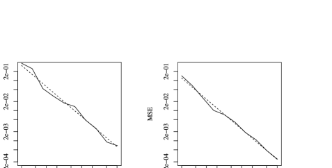
Figure 1: MSE for Example 5.2. Dashed lines are reference lines proportional to $N^{-1}$.

In Figure 1, we show the results for $l=10$, with the choices $K=1$ and $K=4$, that is, with $t^{\ast}=1/10$ and $t^{\ast}=4/10$, respectively. In both case, we observe the asymptotic relation $\operatorname{MSE}\sim N^{-1}$ predicted by Theorem 4.18. The MSE is slightly lower when $t^{\ast}$ is closer to the middle of the interval $[0,1]$ [case (b)] as compared to the situation when $t^{\ast}$ is close to the boundary [case (a)]. Intuitively, one would expect such an effect, as in the latter case the forward process can only accumulate a considerably smaller variance as compared to the reverse process. However, it should be noted that the effect is rather small.

Example 5.3.

Let us consider the stock price $S_{t}$ in a Heston model: $X_{t}:=(S_{t},v_{t})$, that is, the stock price together with its (stochastic) volatility satisfies the stochastic differential equation

$$dS_{t} = \mu S_{t}\,dt+\sqrt{v_{t}}S_{t}\,dB^{1}_{t},$$

$$dv_{t} = (\gamma v_{t}+\beta)\,dt+\xi\sqrt{v_{t}}\bigl{(}\rho\,dB^{1}_{t}+\sqrt{1-\rho^{2}}\,dB^{2}_{t}\bigr{)}.$$

We have

$$a(s,x)=\pmatrix{\mu x^{1}\vspace*{2pt}\cr\gamma x^{2}+\beta},\qquad\sigma(s,x)=\pmatrix{\sqrt{x^{2}}x^{1}&0\vspace*{2pt}\cr\xi\sqrt{x^{2}}\rho&\xi\sqrt{x^{2}}\sqrt{1-\rho^{2}}}.$$

As this process is time-homogeneous, we have $\widetilde{\sigma}=\sigma$, and the remaining coefficients of the SDE for the reverse process are given by

$$\alpha(s,x)=\pmatrix{\bigl{(}2x^{2}+\rho\xi-\mu\bigr{)}x^{1}\vspace*{2pt}\cr(\rho\xi-\gamma)x^{2}+\xi^{2}-\beta},\qquad c(s,x)=x^{2}+\rho\xi-\mu-\gamma.$$

As path-dependent functional we consider the realized variance of the stock-price, that is, for a grid as above we consider

$$g(x_{1},\ldots,x_{l-1},x_{l}):=\sum_{i=1}^{l-1}\bigl{(}\log\bigl{(}x^{1}_{i+1}\bigr{)}-\log\bigl{(}x^{1}_{i}\bigr{)}\bigr{)}^{2}.$$

(Dependence of the functional $g$ on the final value $y$ obviously changes nothing in the theorems of Sections 3 and 4.) We choose $T=1/12$ and $l=30$. This time, however, we only condition on the value of the stock component at final time $T$. For the calculations, we use the following, arbitrarily chosen parameters: $\mu=0.05$, $\gamma=-0.15$, $\beta=-0.045$, $\xi=0.3$, $\rho=-0.7$. The initial stock price and the initial variance were set to $S_{0}=10$ and $v_{0}=0.25$, respectively. Moreover, the realized variance was computed conditionally on $S_{T}=12$, and we choose the standard normal density for $\varphi$, despite Condition 4.20.

Contrary to Example 5.2, we cannot produce samples from the exact distributions of either the forward or the reverse processes $X_{t}$ or $(Y_{t},\mathcal{Y}_{t})$. Thus, we approximate the corresponding paths using the Euler–Maruyama scheme on a uniform grid with mesh $h=\min(1/360,\sqrt{0.05/N})$, so that the MSE for the solution of the corresponding SDE is itself $\mathcal{O}(N^{-1})$, implying that the asymptotic order of the MSE of our quantity of interest is not affected by the numerical approximation of the forward and backward processes. Moreover, evaluation of the functional $g$ is quite costly due to the numerous calls of the $\log$-function. Thus, we use the cut-off procedure introduced above, so that the individual terms in the double sum are only included when the value of the kernel $K_{\varepsilon}$ is larger than $\eta=10^{-3}$. The main parameters of the forward-reverse algorithm are chosen as $M=N$ and $\varepsilon_{N}=(4N)^{-0.4}$, so that we are in the regime of Theorem 4.21.

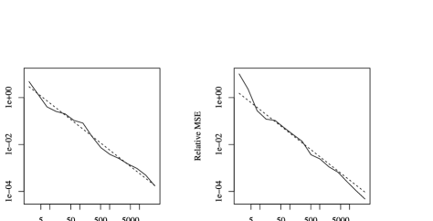
Figure 2: Relative MSE for Example 5.3. Dashed lines are reference lines proportional to $N^{-1}$.

The numerical results in Figure 2 confirm the rate of convergence for the MSE established in Theorem 4.21. Again, there is no significant advantage of choosing $t^{\ast}$ in the middle of the relevant interval $[0,T]$. The “exact” reference value was computed using the forward-reverse algorithm with very large $N$, corresponding small $\varepsilon$ and a very fine grid for the Euler scheme. Note that Figure 2 depicts the “relative MSE,” that is, the MSE normalized by the squared reference value.

References

- Aronson (1967) {barticle}[mr] \bauthor\bsnmAronson, \bfnmD. G.\binitsD. G. (\byear1967). \btitleBounds for the fundamental solution of a parabolic equation. \bjournalBull. Amer. Math. Soc. (N.S.) \bvolume73 \bpages890–896. \bidissn=0002-9904, mr=0217444 \bptokimsref\endbibitem
- Beskos, Papaspiliopoulos and Roberts (2006) {barticle}[mr] \bauthor\bsnmBeskos, \bfnmAlexandros\binitsA., \bauthor\bsnmPapaspiliopoulos, \bfnmOmiros\binitsO. and \bauthor\bsnmRoberts, \bfnmGareth O.\binitsG. O. (\byear2006). \btitleRetrospective exact simulation of diffusion sample paths with applications. \bjournalBernoulli \bvolume12 \bpages1077–1098. \biddoi=10.3150/bj/1165269151, issn=1350-7265, mr=2274855 \bptokimsref\endbibitem
- Beskos et al. (2008) {barticle}[mr] \bauthor\bsnmBeskos, \bfnmAlexandros\binitsA., \bauthor\bsnmRoberts, \bfnmGareth\binitsG., \bauthor\bsnmStuart, \bfnmAndrew\binitsA. and \bauthor\bsnmVoss, \bfnmJochen\binitsJ. (\byear2008). \btitleMCMC methods for diffusion bridges. \bjournalStoch. Dyn. \bvolume8 \bpages319–350. \biddoi=10.1142/S0219493708002378, issn=0219-4937, mr=2444507 \bptokimsref\endbibitem
- Bladt and Sørensen (2012) {bmisc}[author] \bauthor\bsnmBladt, \bfnmMogens\binitsM. and \bauthor\bsnmSørensen, \bfnmMichael\binitsM. (\byear2012). \bhowpublishedSimple simulation of diffusion bridges with application to likelihood inference for diffusions. Preprint. \bptokimsref\endbibitem
- Bolhuis et al. (2002) {barticle}[pbm] \bauthor\bsnmBolhuis, \bfnmPeter G.\binitsP. G., \bauthor\bsnmChandler, \bfnmDavid\binitsD., \bauthor\bsnmDellago, \bfnmChristoph\binitsC. and \bauthor\bsnmGeissler, \bfnmPhillip L.\binitsP. L. (\byear2002). \btitleTransition path sampling: Throwing ropes over rough mountain passes, in the dark. \bjournalAnnu. Rev. Phys. Chem. \bvolume53 \bpages291–318. \biddoi=10.1146/annurev.physchem.53.082301.113146, issn=0066-426X, pii=082301.113146, pmid=11972010 \bptokimsref\endbibitem
- Cattiaux and Mesnager (2002) {barticle}[mr] \bauthor\bsnmCattiaux, \bfnmPatrick\binitsP. and \bauthor\bsnmMesnager, \bfnmLaurent\binitsL. (\byear2002). \btitleHypoelliptic non-homogeneous diffusions. \bjournalProbab. Theory Related Fields \bvolume123 \bpages453–483. \biddoi=10.1007/s004400100194, issn=0178-8051, mr=1921010 \bptokimsref\endbibitem
- Delyon and Hu (2006) {barticle}[mr] \bauthor\bsnmDelyon, \bfnmBernard\binitsB. and \bauthor\bsnmHu, \bfnmYing\binitsY. (\byear2006). \btitleSimulation of conditioned diffusion and application to parameter estimation. \bjournalStochastic Process. Appl. \bvolume116 \bpages1660–1675. \biddoi=10.1016/j.spa.2006.04.004, issn=0304-4149, mr=2269221 \bptokimsref\endbibitem
- Hairer, Stuart and Voss (2009) {bincollection}[mr] \bauthor\bsnmHairer, \bfnmMartin\binitsM., \bauthor\bsnmStuart, \bfnmAndrew\binitsA. and \bauthor\bsnmVoss, \bfnmJochen\binitsJ. (\byear2009). \btitleSampling conditioned diffusions. In \bbooktitleTrends in Stochastic Analysis. \bseriesLondon Mathematical Society Lecture Note Series \bvolume353 \bpages159–185. \bpublisherCambridge Univ. Press, \blocationCambridge. \bidmr=2562154 \bptokimsref\endbibitem
- Hairer, Stuart and Voss (2011) {barticle}[mr] \bauthor\bsnmHairer, \bfnmMartin\binitsM., \bauthor\bsnmStuart, \bfnmAndrew M.\binitsA. M. and \bauthor\bsnmVoss, \bfnmJochen\binitsJ. (\byear2011). \btitleSampling conditioned hypoelliptic diffusions. \bjournalAnn. Appl. Probab. \bvolume21 \bpages669–698. \biddoi=10.1214/10-AAP708, issn=1050-5164, mr=2807970 \bptokimsref\endbibitem
- Haussmann and Pardoux (1986) {barticle}[mr] \bauthor\bsnmHaussmann, \bfnmU. G.\binitsU. G. and \bauthor\bsnmPardoux, \bfnmÉ.\binitsÉ. (\byear1986). \btitleTime reversal of diffusions. \bjournalAnn. Probab. \bvolume14 \bpages1188–1205. \bidissn=0091-1798, mr=0866342 \bptokimsref\endbibitem
- Kusuoka and Stroock (1985) {barticle}[mr] \bauthor\bsnmKusuoka, \bfnmS.\binitsS. and \bauthor\bsnmStroock, \bfnmD.\binitsD. (\byear1985). \btitleApplications of the Malliavin calculus. II. \bjournalJ. Fac. Sci. Univ. Tokyo Sect. IA Math. \bvolume32 \bpages1–76. \bidissn=0040-8980, mr=0783181 \bptokimsref\endbibitem
- Lin, Chen and Mykland (2010) {barticle}[mr] \bauthor\bsnmLin, \bfnmMing\binitsM., \bauthor\bsnmChen, \bfnmRong\binitsR. and \bauthor\bsnmMykland, \bfnmPer\binitsP. (\byear2010). \btitleOn generating Monte Carlo samples of continuous diffusion bridges. \bjournalJ. Amer. Statist. Assoc. \bvolume105 \bpages820–838. \biddoi=10.1198/jasa.2010.tm09057, issn=0162-1459, mr=2724864 \bptokimsref\endbibitem
- Lyons and Zheng (1990) {barticle}[mr] \bauthor\bsnmLyons, \bfnmT. J.\binitsT. J. and \bauthor\bsnmZheng, \bfnmW. A.\binitsW. A. (\byear1990). \btitleOn conditional diffusion processes. \bjournalProc. Roy. Soc. Edinburgh Sect. A \bvolume115 \bpages243–255. \biddoi=10.1017/S030821050002062X, issn=0308-2105, mr=1069520 \bptokimsref\endbibitem
- Milstein, Schoenmakers and Spokoiny (2004) {barticle}[mr] \bauthor\bsnmMilstein, \bfnmGrigori N.\binitsG. N., \bauthor\bsnmSchoenmakers, \bfnmJohn G. M.\binitsJ. G. M. and \bauthor\bsnmSpokoiny, \bfnmVladimir\binitsV. (\byear2004). \btitleTransition density estimation for stochastic differential equations via forward-reverse representations. \bjournalBernoulli \bvolume10 \bpages281–312. \biddoi=10.3150/bj/1082380220, issn=1350-7265, mr=2046775 \bptokimsref\endbibitem
- Milstein, Schoenmakers and Spokoiny (2007) {barticle}[mr] \bauthor\bsnmMilstein, \bfnmG. N.\binitsG. N., \bauthor\bsnmSchoenmakers, \bfnmJ. G. M.\binitsJ. G. M. and \bauthor\bsnmSpokoiny, \bfnmV.\binitsV. (\byear2007). \btitleForward and reverse representations for Markov chains. \bjournalStochastic Process. Appl. \bvolume117 \bpages1052–1075. \biddoi=10.1016/j.spa.2006.12.002, issn=0304-4149, mr=2340879 \bptokimsref\endbibitem
- Milstein and Tretyakov (2004) {barticle}[mr] \bauthor\bsnmMilstein, \bfnmG. N.\binitsG. N. and \bauthor\bsnmTretyakov, \bfnmM. V.\binitsM. V. (\byear2004). \btitleEvaluation of conditional Wiener integrals by numerical integration of stochastic differential equations. \bjournalJ. Comput. Phys. \bvolume197 \bpages275–298. \biddoi=10.1016/j.jcp.2003.12.001, issn=0021-9991, mr=2061247 \bptokimsref\endbibitem
- Papaspiliopoulos and Roberts (2012) {bincollection}[mr] \bauthor\bsnmPapaspiliopoulos, \bfnmOmiros\binitsO. and \bauthor\bsnmRoberts, \bfnmGareth\binitsG. (\byear2012). \btitleImportance sampling techniques for estimation of diffusion models. In \bbooktitleStatistical Methods for Stochastic Differential Equations. \bseriesMonogr. Statist. Appl. Probab. \bvolume124 \bpages311–340. \bpublisherCRC Press, \blocationBoca Raton, FL. \biddoi=10.1201/b12126-5, mr=2976985 \bptokimsref\endbibitem
- Rogers and Williams (2000) {bbook}[mr] \bauthor\bsnmRogers, \bfnmL. C. G.\binitsL. C. G. and \bauthor\bsnmWilliams, \bfnmDavid\binitsD. (\byear2000). \btitleDiffusions, Markov Processes, and Martingales. Vol. 2: Itô Calculus. \bpublisherCambridge Univ. Press, \blocationCambridge. \bidmr=1780932 \bptokimsref\endbibitem
- Spivakovskaya, Heemink and Schoenmakers (2007) {barticle}[mr] \bauthor\bsnmSpivakovskaya, \bfnmD.\binitsD., \bauthor\bsnmHeemink, \bfnmA. W.\binitsA. W. and \bauthor\bsnmSchoenmakers, \bfnmJ. G. M.\binitsJ. G. M. (\byear2007). \btitleTwo-particle models for the estimation of the mean and standard deviation of concentrations in coastal waters. \bjournalStoch. Environ. Res. Risk Assess. \bvolume21 \bpages235–251. \biddoi=10.1007/s00477-006-0059-0, issn=1436-3240, mr=2339199 \bptokimsref\endbibitem
- Stinis (2011) {barticle}[mr] \bauthor\bsnmStinis, \bfnmPanos\binitsP. (\byear2011). \btitleConditional path sampling for stochastic differential equations through drift relaxation. \bjournalCommun. Appl. Math. Comput. Sci. \bvolume6 \bpages63–78. \biddoi=10.2140/camcos.2011.6.63, issn=1559-3940, mr=2836693 \bptokimsref\endbibitem
- Stuart, Voss and Wiberg (2004) {barticle}[mr] \bauthor\bsnmStuart, \bfnmAndrew M.\binitsA. M., \bauthor\bsnmVoss, \bfnmJochen\binitsJ. and \bauthor\bsnmWiberg, \bfnmPetter\binitsP. (\byear2004). \btitleFast communication conditional path sampling of SDEs and the Langevin MCMC method. \bjournalCommun. Math. Sci. \bvolume2 \bpages685–697. \bidissn=1539-6746, mr=2119934 \bptokimsref\endbibitem