Magnetic Systems Triggering the M6.6-class Solar Flare in NOAA Active Region 11158

Abstract

We report a detailed event analysis on the M6.6-class flare in the active region (AR) NOAA 11158 on 2011 February 13. AR 11158, which consisted of two major emerging bipoles, showed prominent activities including one X- and several M-class flares. In order to investigate the magnetic structures related to the M6.6 event, particularly the formation process of a flare-triggering magnetic region, we analyzed multiple spacecraft observations and numerical results of a flare simulation. We observed that, in the center of this quadrupolar AR, a highly sheared polarity inversion line (PIL) was formed through proper motions of the major magnetic elements, which built a sheared coronal arcade lying over the PIL. The observations lend support to the interpretation that the target flare was triggered by a localized magnetic region that had an intrusive structure, namely a positive polarity penetrating into a negative counterpart. The geometrical relationship between the sheared coronal arcade and the triggering region was consistent with the theoretical flare model based on the previous numerical study. We found that the formation of the trigger region was due to a continuous accumulation of the small-scale magnetic patches. A few hours before the flare occurrence, the series of emerged/advected patches reconnected with a preexisting fields. Finally, the abrupt flare eruption of the M6.6 event started around 17:30 UT. Our analysis suggests that, in a triggering process of a flare activity, all magnetic systems of multiple scales, not only the entire AR evolution but also the fine magnetic elements, are altogether involved.

1 Introduction

It is now widely believed that solar flares and resultant various eruptions are massive explosions with the help of magnetic reconnection. On this issue, many observational and theoretical studies have been carried out. Large-scale sunspot motions produce strong magnetic shear (Hagyard et al., 1984) and sharp magnetic gradient (Schrijver, 2007). The nonpotentiality in an active region (AR) is thus achieved and, through this process, free energy is stored in the corona. For starting the release of the stored energy, the existence of driving mechanism is thought to be necessary. Such mechanism includes emerging flux (Heyvaerts et al., 1977; Feynman & Martin, 1995; Chen & Shibata, 2000), converging motion and flux cancellation (van Ballegooijen & Martens, 1989; Moore et al., 2001) at the polarity inversion line (PIL). Therefore, we can understand flares as the phenomena that the stored magnetic free energy in the corona is released through instability and magnetic reconnection, which are triggered by some mechanism. However, the causal interaction among the magnetic structures and the resultant process of flares still remained unclear.

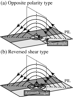
Figure 1: Schematic illustration of the two different types of flare onset suggested by Kusano et al. (2012): (a) opposite polarity (OP) type and (b) reversed shear (RS) type. In both cases, coronal arcade fields lying over the PIL and the local triggering field (emerging flux) are shown by curved thin arrows, while photospheric magnetic fields are indicated by lighter (positive) and darker (negative) hatches. The shear angle of the overlying arcade and the azimuth angle of the triggering field are the parameters that characterize the magnetic configuration. Both angles are measured counterclockwise from the axis normal to the PIL (thick arrows).

Recently, a systematic study of three-dimensional magnetohydrodynamic (MHD) simulations in terms of the flare-triggering mechanisms has been performed by Kusano et al. (2012). They modeled the preexisting coronal arcade overlying the PIL of an AR and a triggering field injected at the bottom boundary. By varying the shear angle of the coronal arcade and the azimuth angle of the injected flux, they systematically surveyed the conditions of the flare onset. As a result, it is found that there are two different types for the flare onset depending on the azimuth angle of the injected flux (Figure 1). One is the opposite-polarity (OP) case, where the injected bipole on the PIL has an opposite orientation to the overlying arcade (Panel a), and the other is the reversed-shear (RS) case, where the azimuth of the bipole is sheared in a reversed sense to the arcade (Panel b). In addition, Kusano et al. (2012) analyzed the observational data of two major flares, an X3.4-class flare on 2006 December 13 in NOAA AR 10930 and an M6.6 flare on 2011 March 13 in AR 11158, and compared these observations with their numerical results. They found that the magnetic configuration and the location of preflare brightening in the X3.4 flare are suitable for the OP-type case, while those in the M6.6 flare are for the RS case.

As for observational studies, the next targets should be the formation process of flare trigger and its interaction with coronal arcades that drives a resultant eruption. In the calculations by Kusano et al. (2012), the flare trigger was simply given in the form of a local flux emergence at the bottom boundary that corresponds to OP- or RS-type configuration. In the actual Sun, however, such a magnetic configuration could be achieved through a variety of dynamic processes including small flux emergence. Recent progress of spatially- and temporally-resolved observations will contribute to the further understanding of trigger development in the preflare phase as well as the whole AR evolution and the consequent eruption.

In this paper, we present a detailed event analysis on the M6.6-class flare occurred on 2011 February 13 in NOAA AR 11158, which was briefly reported in Kusano et al. (2012). Here, we use observational data of this AR taken by multiple spacecrafts, along with the nonlinear force-free field (NLFFF) extrapolation and numerical results of a flare simulation. The targets of this paper are (1) the overall development of the magnetic fields in AR 11158 before the M6.6 flare, (2) the formation process of the flare-triggering region that initiates the M flare, and (3) the evolution of the M flare in the main phase. The rest of the paper proceeds as follows. In Section 2, we introduce observations of AR 11158 and data reduction processes. The obtained magnetic field configurations and the formation of the flare trigger are shown in Sections 3 and 4, respectively. Then, in Section 5, we compare observational results of the M flare with numerical simulations by Kusano et al. (2012). Discussion and summary are presented in Sections 6 and 7, respectively.

2 Observations and Data Reductions

2.1 AR 11158 and the M6.6-class Flare

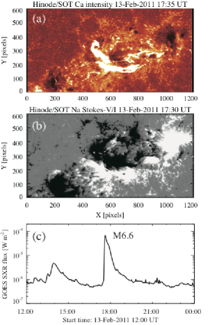
Figure 2: The M6.6-class flare in NOAA AR 11158. (a) Ca intensity map at 17:35 UT and (b) Na Stokes-V/I image at 17:30 UT on 2011 February 13, observed by Hinode/SOT. (c) GOES-15 soft X-ray flux of $1.0$–$8.0\ {\rm\AA}$ channel (1-min cadence).

The target flare of this study is the M6.6-class event on 2011 February 13 in NOAA AR 11158 (see Figure 2). This AR appeared on the southern hemisphere on 2011 February and was composed of two major emerging bipoles. Since the whole evolution of this AR, from its birth to the flares, occurred in the near side of the Sun, we can particularly investigate the evolution history of the magnetic fields related to the flares from its earliest stage. Above the highly sheared PIL located at the center of this quadrupolar region, many flares including one X- and some M-class events were observed. The M6.6 flare broke out around 17:30 UT on February 13, which can be seen in the Geostationary Operational Environmental Satellite (GOES) soft X-ray flux ($1.0$–$8.0\ {\rm\AA}$ channel) in Figure 2c. The M6.6 event here was about 32 hr before the X2.2 flare, the first X-class flare of Solar Cycle 24, which occurred on the same PIL (Schrijver et al., 2011).

In Kusano et al. (2012), they identified a flare-triggering region of the M6.6 event on February 13 and found that the triggering region had an RS configuration. The formation of this trigger, however, still remained unclear. In this study, we focus on the magnetic fields, especially on the formation of the trigger region, by using observational data introduced below.

2.2 Hinode/SOT Data

The Hinode satellite (Kosugi et al., 2007) tracked NOAA AR 11158 from 09:57 UT, February 12, to 09:01 UT, February 19. During this period, the Filtergram (FG) of the Solar Optical Telescope (SOT: Tsuneta et al., 2008) on board Hinode obtained circular polarization (CP) data of Na I D₁ line (5896 Å), shifted by $140\ {\rm m\AA}$ from the line center, which is called Stokes-V/I images hereafter, and intensity data of Ca II H line (3968.5 Å). The time cadence is 5 min for each data, and the original field of view (FoV) is $225.3^{\prime\prime}\times 112.6^{\prime\prime}$ for Stokes-V/I and $183.2^{\prime\prime}\times 108.5^{\prime\prime}$ for Ca data, respectively. The spatial sampling is $0.16^{\prime\prime}$ for Stokes-V/I images and $0.108^{\prime\prime}$ for Ca images. Both data are calibrated through fg_prep procedure included in SolarSoftWare (SSW) package for dark-current subtraction and flat fielding. Then, by taking a cross-correlation between two consecutive images, we reduce small spatial fluctuations. Finally, Ca images are enlarged to fit the size of the Stokes-V/I data and structures in these images are compared.

The Spectro-Polarimeter (SP) of the SOT takes spectrum profiles of two magnetically sensitive Fe I lines at 6301.5 and 6302.5 Å. The SP scan data obtained in the observational period on February 13 have a time cadence of 90–120 min and a spatial sampling of $0.32^{\prime\prime}$. The FoV is basically $164^{\prime\prime}\times 164^{\prime\prime}$; some scans have a lack of spectral data. In this study we use the SOT/SP level2 data, which are the outputs from the inversions using the Milne-Eddington gRid Linear Inversion Network (MERLIN) code (Lites et al., 2007).

2.3 SDO/AIA and HMI Data

The Atmospheric Imaging Assembly (AIA: Lemen et al., 2012) on board the Solar Dynamics Observatory (SDO) continuously observes the coronal dynamics of the whole solar disk at multiple wavelengths. In this study we use the tracked cutout data of AR 11158 with a time cadence of $12\ {\rm s}$ and a pixel size of $0.60^{\prime\prime}$, which are taken from the SDO AIA Get Data page. We also use the magnetogram of the Helioseismic and Magnetic Imager (HMI: Scherrer et al., 2012; Schou et al., 2012) of the same FoV with a time cadence of $45\ {\rm s}$ and a pixel size of $0.50^{\prime\prime}$, along with the vector magnetic field data with a cadence of 12 min, which is cut out from the full disk data using HARP (Turmon et al., 2002, 2010).

2.4 Nonlinear Force-Free Field Data

NLFFF extrapolation is also applied to the vector field data taken by SDO/HMI (Section 2.3) in order to investigate the three-dimensional magnetic structure. In this study, the MHD relaxation method developed by Inoue et al. (2013) is employed to reconstruct the force-free field. The initial and boundary conditions for the iterative calculation are given by a three-dimensional potential field and the preprocessed vector magnetogram. The detailed procedure will be explained in Appendix A.

The NLFFF model covers the domain $L_{x}\times L_{y}\times L_{z}=184.32\times 184.32\times 184.32\ {\rm Mm}^{3}$, which is resolved by $128\times 128\times 128$ grids. The bottom boundary condition is obtained from a $4\times 4$ binning of the original vector magnetogram of $512\times 512$ pixels. The grid size of the NLFFF corresponds to about $1688\ {\rm km}$, i.e., about $2.3^{\prime\prime}$.

3 Magnetic Field Configuration: Preflare State

In this section, we first describe the overall development of the magnetic field in the preflare stage. Then we focus on the magnetic configuration of the possible candidate for the flare trigger of the M6.6-class flare, which was localized in the center of this AR.

3.1 Initial Phase and the Formation of Sheared PIL

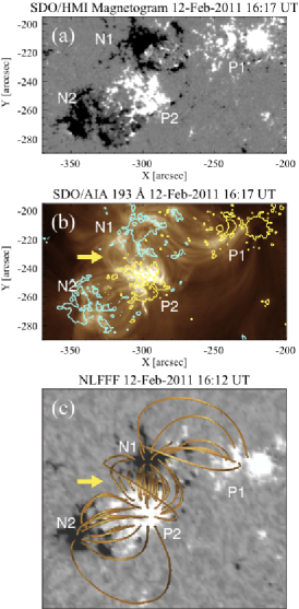
Figure 3: (a) SDO/HMI magnetogram of NOAA AR 11158 taken at 16:17 UT on 2011 February 12, $\sim$1 day before the M6.6-class flare. The grayscale saturates at $\pm 200\ {\rm G}$ and the axes are in arcseconds from disk center. Numbers representing two bipolar pairs (P1–N1 and P2–N2) are overplotted. (b) SDO/AIA 193 Å image at the same time as (a). Contour levels of $\pm 200\ {\rm G}$ are indicated as yellow and turquoise lines. (c) NLFFF calculated from HMI magnetogram. Arrows in Panels (b) and (c) show the coronal arcade connecting N1 and P2.

In its initial phase, AR 11158 was composed of two major emerging fluxes. Figure 3a shows the SDO/HMI magnetogram of this AR at 16:17 UT on February 12, about 1 day before the M6.6-class flare. The first bipole (P1–N1) appeared on the southern hemisphere on February 9, while the second pair (P2–N2) appeared on 10. Both pairs, of which the field strengths were larger than $1000\ {\rm G}$, gradually separated from each other since their births, with increasing flux sourced from a series of minor emergences.

Figure 3b shows the SDO/AIA 193 Å image at the same time as Panel (a). This figure indicates that there were coronal arcades connecting magnetic patches N1 and P2 (indicated by an arrow) as well as arcades connecting P1–N1 and P2–N2. Such arcades are also seen in the NLFFF map, in Panel (c), which is calculated from the HMI magnetogram as a bottom boundary condition. Here one may speculate that the original loops of P1–N1 and P2–N2 conflicted over the PIL between N1 and P2 and made new loops of N1–P2 via magnetic reconnection. The other half of the reconnected loops bridging between P1–N2 may lie above the entire AR, which is not seen in the NLFFF map in Panel (c).

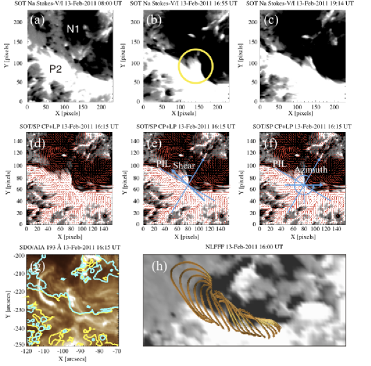
Figure 4: (a–c) Time-development of the PIL between N1 and P2 in Na Stokes-V/I maps taken by Hinode/SOT. White and black represent positive and negative polarities, respectively. One can see that the intrusive magnetic structure is formed along the PIL before the M6.6-class flare starting from 17:30 UT (yellow circle). (d–f) Hinode/SOT SP circular polarization (CP) map before the flare. Linear polarization (LP) that represents transverse field is overplotted as red small bars. The time shown is when the SP scan slit comes to the center of the field of view. Auxiliary lines for measuring the shear and azimuth angles are overplotted in Panels (e) and (f). (g) SDO/AIA 193 Å image at the same time as (d–f), overplotted with field strength contours of $\pm 200\ {\rm G}$. Coronal arcades are across the PIL with a shear, which is also seen in (h) the NLFFF map.

During the evolution of this AR, the southern positive patch P2 continuously moved to the west, while the northern negative patch N1 drifted to the east. Therefore, the coronal arcade N1–P2 was continuously sheared in the counterclockwise direction throughout the whole evolution process (right-handed shear), which can be seen by comparing Figures 3(b) and (c) and Figures 4(g) and (h). Such a continuous shearing strongly indicates the storage of free energy in the corona above the PIL between N1 and P2. On the contrary, P1 and N2 moved slowly and remained almost at the same positions from February 14. Therefore, the large-scale evolution in this AR can be described as the inner two polarities N1 and P2 moved rapidly as if they merged into outer two polarities N2 and P1, respectively, creating a highly sheared PIL between N1 and P2.

3.2 Intrusive Magnetic Structure on the PIL

As the AR developed, N1 and P2 came close to each other and the magnetic gradient across the PIL N1–P2 increased. Figures 4(a–c) are SOT Na Stokes-V/I images, showing the temporal evolution of this PIL. In Panel (a), at 08:00 UT on February 13, there still remained a polarity gap between N1 and P2 patches. In Panel (b), about 30 min before the M6.6-class flare took place, however, the gap had been filled with a positive polarity. Here one may find that an intrusive magnetic structure, where the positive polarity P2 penetrates into the negative polarity N1, has been formed on the PIL (yellow circle). This magnetic structure weakened after the flare finished in Panel (c). Kusano et al. (2012) reported that, from the comparison with flare simulations, this intrusive structure is the flare-triggering region of the M6.6 flare.

Figures 4(d–f) are the SOT/SP map taken at 16:15 UT on February 13. These images show vertical and transverse fields at the photosphere, indicating the precise magnetic configuration around the intrusive structure. In Panel (d), the transverse field (red bars) was highly sheared and was almost along the PIL because of the counterclockwise motion of the both polarities (right-handed shear). The 193 Å image in Panel (g) and the NLFFF map in Panel (h) also show that the overlying coronal arcade connecting N1 and P2 was highly sheared at this time. This sheared PIL had a length of more than $20\ {\rm Mm}$. To estimate the shear angle of the overlying arcade and the azimuth of the local magnetic structure from the PIL, we overplotted auxiliary lines in Panels (e) and (f). Following Figure 1, we measured the shear and azimuth angles, counterclockwise from the normal of the PIL. Here the shear is evaluated from the transverse field, while the azimuth is from the western edge of the intrusive structure. The measured shear angle is $\sim 80^{\circ}$ and the azimuth ranges for $270^{\circ}$–$300^{\circ}$.

From the observations in this section, we see that the large-scale coronal arcade above the PIL satisfies the sufficient conditions for large flares proposed by Hagyard (1990). That is, (1) the shear angle of the coronal arcade is as much as $\sim 80^{\circ}$, (2) the field strength is large enough ($\geq 1000\ {\rm G}$), and (3) the length of the PIL is large enough ($\geq 10\ {\rm Mm}$).

4 Formation of the Intrusive Structure: Flare Trigger

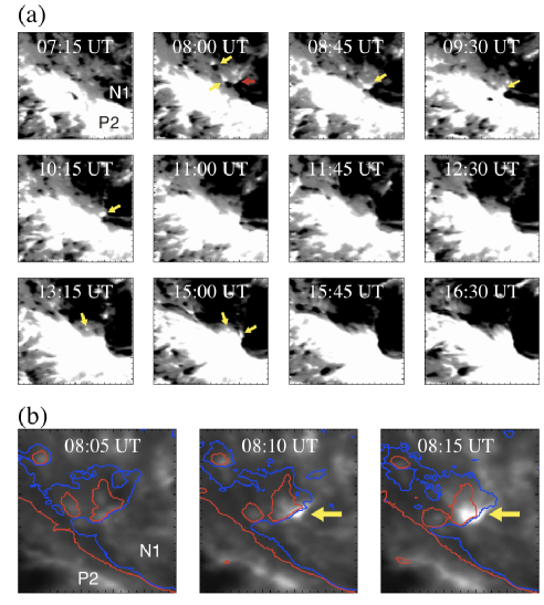
Figure 5: (a) SOT Na Stokes-V/I maps from 07:15 to 16:30 UT, 2011 February 13, indicating the formation of the intrusive structure on the PIL between N1 and P2. Arrows show the small-scale magnetic bipoles that collide into the preexisting polarities. (b) SOT Ca images of the collision event indicated by a red arrow in Panel (a). Red and blue contours show the data number (DN) of the circular polarization $=\pm 20$, respectively. Arrows indicate the Ca brightenings at the collision site of the two polarities.

Figure 5a is the SOT Na Stokes-V/I maps around the intrusive magnetic structure (the flare-triggering region) from 07:15 to 16:30 UT on February 13. Note that there was a temporal gap in the SOT data between 13:15 and 15:00 UT, since, due to the telemetry limitation of the Hinode satellite, the SOT data in this time range was overwritten. As can be seen from Figure 5a, initially at 07:15 UT, there still was a wide gap on the PIL between the two major polarities (N1 and P2) and here the intrusive structure was not evident. As time went on, a series of small-scale magnetic bipoles emerged at the PIL, collided into the major polarities (indicated with arrows), and eventually filled the gapped PIL. Figure 5b is the Ca image of one particular collision event in Panel (a) (shown by a red arrow in 08:00 UT), where a positive patch was advected and conflicted with the preexisting negative polarity (N1). One may see that a Ca brightening became more evident above the collision site, bridging over the both polarities (indicated by arrows). This Ca brightening suggests magnetic reconnection between the advected small magnetic patch and preexisting polarities. We found similar brightenings all the way through the formation of the intrusive magnetic structure. Therefore, we expect that the accumulation of emerged/advected small-scale bipoles is essential for the formation of the intrusive structure in this AR.

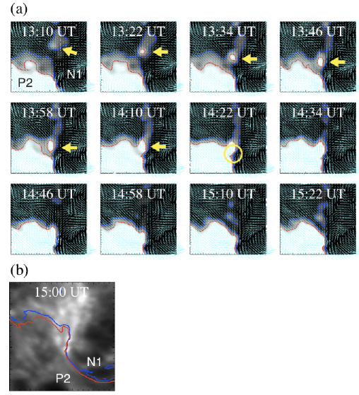
Figure 6: (a) HMI vector magnetogram during 13:10–15:22 UT. Grayscale shows the longitudinal field, while skyblue bars indicate the transverse field. Here the direction of the transverse fields are not indicated. Red and blue lines are the contour level of longitudinal component $=\pm 100\ {\rm G}$, respectively. The small positive patch indicated by arrows collides into the major positive patch P2. At 14:22 UT, the transverse field in the circle connects the colliding positive patch and preexisting negative polarity N1. (b) SOT Ca image around the PIL at 15:00 UT of the same day. Red and blue contours indicate the DN of the circular polarization $=\pm 20$, respectively.

Next, let us focus on the collision event that seems related to the triggering of the M6.6 flare. Before the flare occurrence, there were many emergences and collisions of the patches. One of the collision events that possibly led to the M flare is the case shown in Figure 6. In Panel (a), we plot HMI magnetograms (longitudinal and transverse fields) around the intrusive structure for every 12 minutes from 13:10 to 15:22 UT. Here we do not indicate the direction of the transverse fields (transverse fields are shown by bars instead of arrows), since the small-scale fields we focus on extend only for several pixels in this map and thus the orientation of such fields may have been smoothed out in the inversion process. At 13:10 UT, a positive magnetic patch started to emerge and was then advected southward (indicated with arrows). At 14:22 UT, the positive patch merged into the main positive polarity (P2: intrusive structure), colliding against the preexisting negative polarity (N1). The transverse fields in the yellow circle clearly connect the advected positive patch and the negative polarity, which remains until 14:58 UT. The transverse fields connecting the both fields indicate the magnetic reconnection between the positive flux of the advected patch and the negative flux of the major polarity (N1). In this map, however, only six pixels (a size of a few Mm) in the negative patch (yellow circle) were related to the reconnection. Here, the azimuth angle of the transverse fields, averaged over the six pixels, was measured to be $252^{\circ}$. After the collision of the advected bipoles, the SOT Ca image at 15:00 UT in Figure 6b reveals enhanced brightenings around the PIL.

Here we summarize the observations in this section. The intrusive magnetic structure (the flare-triggering region) was formed through the continuous accumulation of the small-scale emerging bipoles. When the positive patch collided against the preexisting negative field, we observed Ca brightenings above the collision site, which suggests a magnetic reconnection between them. One of the collision events that possibly led to the triggering of the M6.6 flare was observed between 14:00 to 15:00 UT, February 13, more than two hours before the flare occurrence. The azimuth angle of the reconnected transverse field was measured $252^{\circ}$, while its spatial size was only a few Mm.

5 Comparison with Numerical Simulation: M6.6-class Flare

Observations of the magnetic fields related to the M6.6 flare in AR 11158 indicate that the geometrical relationship between the overlying coronal arcade and the intrusive magnetic structure (the flare-triggering region), namely, the shear angle of the arcade (80^∘) and the azimuth of the flare trigger (270^∘ to 300^∘), is consistent with the RS model in Kusano et al. (2012). Thus, in this section, we provide a detailed comparison of the observation with the numerical results of RS model.

The basic setup of the simulation is described in Kusano et al. (2012). Here we show the numerical result with a shear angle of the overlying linear force-free field (LFFF) of 80^∘ and an azimuth of the injected triggering flux of 270^∘, which corresponds to the RS-type configuration. Figure 7 shows the temporal evolution of the simulation. The left column shows the selected magnetic field lines and the current density in the central plane, while the middle column shows the magnetogram with the shift of the field connectivity (red: see Appendix B) and the current density in the lower atmosphere (green).

In the initial state at $t=0.0$, as of Panels (a) and (b), one can see a highly-sheared coronal arcade above the PIL ($y=0$). When the bipolar flux was injected from the bottom boundary, Panels (d) and (e), the current sheet P was formed between the injected flux and the coronal fields, and the primary reconnection proceeded in the current sheet. Due to the reduction of the magnetic flux from the reconnection site P, the force balance among the arcade fields was partially lost, which pulled the ambient arcade fields into the center of the domain and formed a twisted flux rope via the secondary reconnection. In Panel (j), one may see that the twisted flux rope T is detached and erupts upward, creating a vertical current sheet S beneath. (For the detailed illustration of the field lines and current sheets, the reader is referred to Figure 4 of Kusano et al. 2012.) The footpoints of the fields lines that connect to the flux rope T are labeled as F in Panels (h), (j), and (k), while those connecting to the postflare arcade are shown as R.

Compared with the numerical results, SOT Ca images reveal clear consistencies throughout the whole evolution process. At 15:25 UT in Figure 7f, the preflare brightening P’ above the PIL N1–P2, which was also shown as the brightenings in Figure 6b, was comparable to the current sheet P between the injected triggering field and the preexisting coronal arcade. In Panel (i), the flare two-ribbon F’ in the eruptive phase from 17:30 UT, extending along the PIL from the intrusive structure (flare-triggering region), was also well in accordance with the footpoints of the reconnected coronal fields F and of the postflare arcades R in Panel (h). The flare ribbons in the late phase in Panel (k), however, deviated from the observation of the Ca ribbons in Panel (l). In the simulation both ribbons at $y=\pm 0.2$ elongated along the PIL to both positive and negative $x$-directions, while in the actual Sun the ribbons stopped their elongations along the PIL from 17:35 UT.

It should be noted here that the polarities in Panels (i) and (l) show reversals, possibly due to the strong Dopplershifts that correspond to the M flare (Fischer et al., 2012); the black patches in the southern positive polarity were actually positive rather than negative and the white patches in the north were negative. The reversals were also observed above the most distant sunspots P1 and N2.

There is also a difference between the simulation and observation. Here, in the numerical simulation, the flare trigger was given as a simple “emerging flux” with an RS configuration, injected into the domain from the bottom boundary. On the other hand, the observed flare trigger (intrusive structure) was created through a continuous accumulation of emerged/advected bipoles, and the RS-component field was supplied by their magnetic reconnection (see Section 4). These discrepancies between the modeled and actual Sun will be discussed in the next section.

6 Discussion

In the previous sections, we have investigated the evolution of the magnetic fields that caused the M6.6-class flare in NOAA AR 11158, from flux emergence to the eventual eruption, by spacecraft observations and a comparison with the numerical simulation.

AR 11158 was characterized by its two major emerging fluxes P1–N1 and P2–N2 (Figure 3). In this quadrupolar region, the central PIL between N1 and P2 was continuously sheared by the counterclockwise motions of the major polarities N1 and P2, and, through this process, the coronal arcade over this PIL was highly sheared (Figure 4). The observations indicate that the M6.6 flare was triggered by the intrusive magnetic structure that appeared on this PIL. The shear angle of the coronal arcade and the azimuth of the intrusive structure were measured to be 80^∘ and 270^∘–300^∘, respectively, which corresponds to the RS-type model in Kusano et al. (2012). It was also found that the intrusive structure (the flare-triggering region) was formed through the continuous accumulation of the emerged/advected bipoles and their reconnections with the preexisting negative field (Figures 5 and 6). Based on the results above, here we discuss some issues on the magnetic structures that correspond to the flare onset and the resultant eruption.

6.1 Similarities and Differences between Modeled and Actual Sun

In Section 5, we compared the observation with the numerical results of the RS type in Kusano et al. (2012). We found that the Ca preflare brightenings above the triggering region were highly consistent with the numerical results (Figures 7e and f). The brightenings were explained as a current sheet between the localized flare trigger and the overlying coronal arcade.

The structure of the flare ribbons in the simulation was also consistent with the observation (Figures 7h and i). However, the simulated ribbon structure deviated from that in the actual Sun, especially in the late phase (Panels k and l). In the computational domain, the ribbons elongated from the triggering field ($x=0$) to both $x$-directions, because the reconnections among the coronal arcades (given as linear force-free fields: LFFF) occurred successively along the PIL (i.e., the $x$-axis). On the other hand, in the observation, the ribbons stopped their elongations along the PIL, possibly because the region of the highly-sheared arcade with 80^∘ was localized around the flare trigger (the intrusive structure) and the shear outside this region was not so high as $\sim 80^{\circ}$, which inhibited the successive reconnections of the coronal arcades propagating along the PIL. In other words, the non-uniformity of the shear angle in the AR, or, the effect of non-linear force-free fields (NLFFF), limited the elongation of the flare two-ribbons. This story is well in line with the simulation results of the RS type with different shear angles; the flare eruption was observed in the highly-sheared case, while it failed in the weakly-sheared case (compare the cases with azimuth of 270^∘ in Figure 2 of Kusano et al. 2012).

In addition, there was an important difference between the simulation and the observation. In the simulation, the flare trigger was given as a simple “emerging flux” from the bottom boundary. However, the flare trigger of the M6.6 event in AR 11158 was formed through a series of bipolar emergences and their reconnections with the preexisting field. This discrepancy may suggest the possibility that the flare-triggering region in the actual Sun can be achieved through a variety of dynamic processes, while the essential magnetic configuration can be classified into the two simple categories, OP and RS.

Here we comment on the contrast of the time scale between the simulation (Figure 7 left and middle columns) and the observation (right column). If we take $0.4\ {\rm s}$ for a normalizing unit of the time following Kusano et al. (2012), the entire calculation spans only $16\ {\rm s}$, which is three orders of magnitude shorter than the observed time range of the M6.6 flare. In the simulation, the emergence speed of the injected triggering flux is made faster than the actual flux emergence in the Sun ($\sim 1\ {\rm km\ s}^{-1}$) by two orders, in order to reduce the computation time and focus mainly on behaviors after the flux injection (see also Section 4.2 of Kusano et al., 2012). Also, the electrical resistivity in the simulation is set much larger, which may drastically speed up the magnetic reconnection between the injected flux and the overlying arcade. However, since the emergence in the simulation is much slower than the Alfvén velocity, the results after the injection do not depend much on the emergence speed. Plus, although the reconnection proceeds much faster in the computation, we believe that the topological evolution of the magnetic structure in the nonlinear phase is properly solved because the reconnection time is longer than the Alfvén time (dynamical time scale) and is much shorter than the diffusion time.

6.2 Large-scale Magnetic System, Subsurface History, and Successive Flares

In its birth of AR 11158, we observed two major emerging fluxes P1–N1 and P2–N2 (see Figure 3). The motions of the quadrupole were described as two inner polarities N1 and P2 moving rapidly as if they merged into rather-stable outer polarities N2 and P1, respectively. The relative motion of N1 and P2 built a highly-sheared PIL in the center of the AR and thus the magnetic free energy was stored in the corona. Finally, the M6.6 flare, which had an RS configuration, broke out above this PIL.

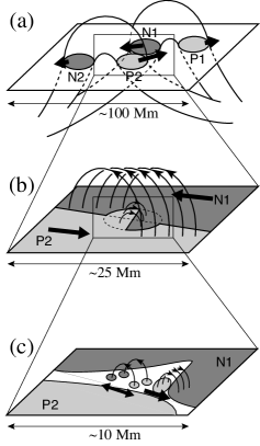
Figure 8: Schematic illustration of the magnetic structures in multiple scales that are involved in the M6.6-class flare in NOAA AR 11158. (a) Ellipses on the plane (photosphere) indicate the two major bipoles, P1–N1 and P2–N2. Lighter and darker shadows mean the positive and negative polarities, respectively. Tubes above and below the photosphere show the expected flux tubes that compose this AR. (b) Closeup of the PIL between N1 and P2. Relative motions in both sides of the PIL shear the overlying coronal arcade, while, in the core of the PIL, flare-triggering region (intrusive structure) with the RS-component flux appears. (c) The formation of the triggering region is illustrated. Small-scale bipoles emerge in the gapped PIL, and the positive patch is advected to collide into N1 polarity, forming RS flux through magnetic reconnection.

From the point of view that the flare is a relaxation process leading to a lower energy state, along with the proper motions of the quadrupole, this AR is strongly reminiscent of the history that a single flux tube emerged from the deeper convection zone split into two by some perturbations and these split tubes appeared at the neighboring locations at the visible surface (see also Chintzoglou & Zhang, 2013). Figure 8a illustrates this concept. Here the two flux tubes that appear at the photosphere (P1–N1 and P2–N2) share the common roots below the surface. The relative motion of N1 and P2 and the resultant M flare can be explained by the rising of this large-scale magnetic system as a whole. Therefore, to understand the cause of flares, it is surely important to investigate the subsurface magnetic fields by helioseismology (e.g., Ilonidis et al., 2011; Toriumi et al., 2013) and numerical approaches (e.g., Toriumi & Yokoyama, 2010, 2012).

The flare simulation in Section 5 showed that the filament eruption of the M flare on February 13, 2011, was caused through the collapse of the coronal arcades (Figure 7j). This situation is in accordance with the tether-cutting model suggested by Moore et al. (2001) and the magnetic structure is consistent with the classical CSHKP model (Carmichael, 1964; Sturrock, 1966; Hirayama, 1974; Kopp & Pneuman, 1976). Also, the numerical results predict that, as the filament erupted into the space, there remained a postflare arcade beneath the detached filament (R in Figure 7j), which is a remnant of the reconnected coronal arcades. Liu et al. (2012) found that the photospheric horizontal fields increased drastically after the M flare. They discussed in favor of the tether-cutting reconnection that the upper part of the reconnected arcades erupted outward, while the lower part contributed to enhance the photospheric fields. The lower fields may be the same as the postflare arcade in the simulation results of our study.

After the M6.6 event, the newly created postflare arcade connecting N1 and P2 was sheared further by the continuous photospheric motions. We believe that the continuous motions were also caused by the large-scale flux system, namely, the emergence of the spilt tubes (Figure 8a). The highly-sheared coronal arcade was thus formed again along the same PIL between N1–P2, which may be the overlying arcade in the X2.2 flare that occurred on February 15. Wang et al. (2012) also observed the enhancement of the photospheric horizontal fields after the X flare, explaining that the X event was similarly caused by the tether-cutting reconnection (see also Sun et al., 2012).

A series of flares along the central PIL in AR 11158, including X2.2, M6.6, and many C-class events, indicate that (1) successive flares in a single AR are the way to relax the continuous shearing of the magnetic fields by the photospheric motions, or, by the large-scale flux emergence of the whole magnetic system, (2) the timing of each flare is determined by the appearance of a flare trigger, and (3) the magnitude of each event depends on the conditions of the event, e.g., the amount of coronal flux aligned on the PIL, the shear angle of the coronal arcades, and the azimuth angle of the triggering field. And, the large-scale magnetic system emerged from the subsurface layer is thus important for the successive flares.

6.3 Multiscalability of the Magnetic Systems

As was seen in the observations, magnetic structures in AR 11158 extended widely over multiple spatial scales, ranging from the entire length of the AR of the order of 100 Mm to the size of the RS-component flux of a few Mm. Also the time scale distributed from days to hours.

Figure 8a shows the largest-scale structure in this AR, i.e., the double bipolar systems P1–N1 and P2–N2. The size of each emergence extended more than 40 Mm and the development lasted for several days. As was discussed in Section 6.2, the proper motions of the quadrupole can be explained as the emergence of the two split tubes that share the common roots. If this is the case, the series of flares above the PIL can be understood as the process that the split flux tubes recovered their original shape (a single tube) when they rose into the corona, where the gas pressure is less dominant.

The M6.6-class flare analyzed in this study was found to be triggered by the smaller-scale magnetic field. Figure 8b shows a closeup of the PIL between N1 and P2, where these polarities sheared the coronal arcade by their relative motions. It was found that, the intrusive magnetic structure of $\sim 5\ {\rm Mm}$, localized in the center of the PIL, was a possible flare trigger. From Figures 4a–c, one can see the lifetime of the intrusive structure is less than a half day, or about 10 hours.

The formation of the intrusive structure on the PIL (the flare-triggering region) was caused by much smaller-scale events. Figure 8c illustrates the formation process of the intrusive structure. First, small-scale bipoles of the size of a few Mm emerged continuously in the middle of the gapped PIL. Some of the positive patches were then advected to the west and finally collided into the preexisting negative field N1 (see Figure 5a). The time scale of each advection/collision was about, or less than 1 hour. At the same time, we observed brightenings in the Ca image (Figure 5b), which indicates the reconnection between the advected patch and the preexisting fields. Magnetic flux of RS component was thus achieved.

The multiscalability of the magnetic fields both in spatial and temporal scales indicates that, even in the large-scale events like flares and resultant eruptions, smaller-scale physics plays an important role in driving the entire system. This may also indicate that, for the flare prediction, we have to deal with the short-lived flare trigger of the time scale of a few hours. Therefore, to completely understand the nature of flares, further studies that simultaneously handle the small-scale/short-term flare trigger and the large-scale/long-term evolution of the entire AR are required.

6.4 Categorization of Flare-Productive ARs

As discussed above, the large flares in AR 11158 occurred mainly on the continuously-sheared PIL, which is formed by a relative motion of two major emerging bipoles. Our explanation of the flares is that they are the relaxation process of a single flux tube, which has been split into two tubes by some dynamics in the convection zone, restoring its original geometry (Figure 8a). And one of these flares, the M6.6 event, was found to be consistent with the RS-type model.

On the contrary, NOAA AR 10930, also a flare-productive region sourcing several X-class events, basically consisted of a single bipole (Kubo et al., 2007). The long-term evolution in this AR was that the southern positive polarity passed by the large, northern negative polarity from west to east, while the positive polarity itself rotated counterclockwise, forming a highly sheared PIL. Kusano et al. (2012) focused on this PIL and found that the X3.4-class flare on 2006 December 13 can be explained by the OP model. The possible scenario of this AR is that, through a series of flares, the twisted flux tube forming this region expelled its internal helicity (or shear) into the space for relaxation to a lower energy state.

From these examples, we can see that there exist some scenarios for the flare-productive ARs. The flux tubes of complex, multipolar regions such as AR 11158 may have suffered severe interruptions during their ascents in the convection zone. And thus, they may try to restore their original shapes via flares as a mean of relaxation (see also Poisson et al., 2013). Meanwhile, the tubes of simpler, perhaps bipolar regions such as AR 10930 may have been tightly twisted under the visible surface. As they appear into the atmosphere, the twisted tubes may lighten up their helicities in the form of flares.

The above categorizations of the ARs, along with the triggering mechanisms of OP and RS, can be used to classify the flaring events. However, it is not clear whether complex, multipolar regions are in favor of the RS model, and simple, bipolar regions are for OP. Statistical studies may help to understand the relationship among these elements.

7 Summary

NOAA AR 11158 was a flare-productive region, mainly composed of two large-scale emerging fluxes. Because of the relative motions of the two inner polarities, a highly sheared PIL was created in the center of this AR, which then sheared the coronal arcade lying over the PIL. Based on the observations, we here interpret that the M6.6-class flare on 2011 February 13 was triggered by a localized magnetic region that had an intrusive topology, the positive polarity penetrating into the negative side. The geometrical relationship between the flare trigger and the coronal arcade was in favor of the RS scenario of Kusano et al. (2012). The shear angle of the arcade and the azimuth angles of the flare trigger were measured to be $80^{\circ}$ and $270^{\circ}$–$300^{\circ}$, respectively, which agrees with the RS model. We found that the development of the flare-triggering region was due to a series of small-scale emerging bipoles, a few hours before the flare occurrence. Through magnetic reconnections between advected positive patch and the preexisting negative field, magnetic flux of the RS component was thus achieved. Finally, after the triggering region was formed, the M flare started at around 17:30 UT. These results indicate that a wide spectrum of magnetic systems, ranging from the large-scale evolution of the entire AR to the small-scale accumulation of magnetic elements, is altogether involved in a flare activity.

Appendix A Initial and Boundary Conditions for the NLFFF Extrapolation

To obtain the initial and boundary conditions for the NLFFF extrapolation, we decompose the magnetic field normal to the solar surface $B_{n}$ to the averaged component $\bar{B}_{n}$ and the undulate component $b=B_{n}-\bar{B}_{n}$. Assuming a periodic condition for the horizontal coordinates, we calculate a potential magnetic field for $b$ in terms of the Fourier transform

$$\mbox{\boldmath$B$}=\sum_{m,n}\tilde{\mbox{\boldmath$b$}}_{(m,n)}\exp{(ik_{m}x+ik_{n}y-|k|z)},$$ (A1)

where $k_{m}=2\pi m/L_{x}$, $k_{n}=2\pi n/L_{y}$, $|k|=\sqrt{k_{m}^{2}+k_{n}^{2}}$, $m=-n_{x}/2,\cdots,-1,1,\cdots,n_{x}/2$, and $n=-n_{y}/2,\cdots,-1,1,\cdots,n_{y}/2$, respectively. The complex Fourier coefficient vector $\tilde{\mbox{\boldmath$b$}}_{(m,n)}$ consists of $\tilde{b}_{x(m,n)}=-ik_{m}\tilde{b}/|k|$, $\tilde{b}_{y(m,n)}=-ik_{n}\tilde{b}/|k|$, and $\tilde{b}_{z(m,n)}=\tilde{b}$ that is a Fourier transform of $b$.

In order to compensate the excess magnetic flux $\bar{B}_{n}S_{b}$ on the bottom boundary, we add a small bias field $-\bar{B}_{n}S_{b}/S_{a}$ to the normal component of magnetic field on all the lateral and top boundaries, where $S_{b}$ and $S_{a}$ are the area of the bottom boundary and the total area of the lateral and top boundaries, respectively. Then, we derive the potential field $\mbox{\boldmath$B$}=-\nabla\Phi$, solving the Poisson equation $\nabla^{2}\Phi=0$ numerically. This potential field is used as the initial condition for the NLFFF calculation. Incrementally imposing the transverse components of the observed vector magnetogram onto the bottom boundary, the NLFFF is iteratively calculated based on the MHD equation. The normal components on all the boundaries are fixed, while the transverse components on the lateral and top boundaries are solved under the condition that these boundaries are perfectly conductive.

Appendix B Shift of the Field Connectivity

In the middle column of Figure 7, we plot with red contours the shift of the field connectivity from the initial linear force-free condition. From each point of the bottom boundary, $\mbox{\boldmath$x$}_{0}$, the end point of the field line at the time $t$ is traced, which is denoted as $\mbox{\boldmath$x$}_{1}(\mbox{\boldmath$x$}_{0};t)$. In this map, the red contour indicates the shift of the end point at $t$ from the initial force-free state, $|\mbox{\boldmath$x$}_{1}(\mbox{\boldmath$x$}_{0};t)-\mbox{\boldmath$x$}_{1}(\mbox{\boldmath$x$}_{0};0)|$, at each location $\mbox{\boldmath$x$}_{0}$. If this value is larger, the field line traced from that position has reconnected with another field line which was initially located farther.

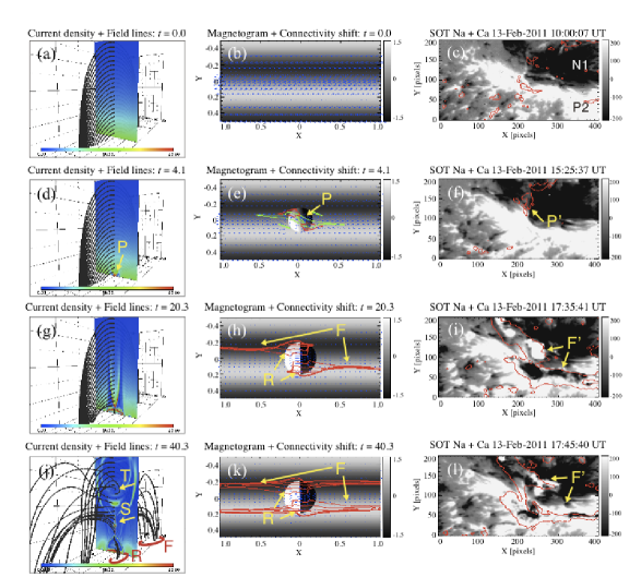
Figure 7: (Left) Numerical results of the RS-type simulation. Selected field lines passing through the vertical axis $x=y=0$ and current density in the vertical plane $x=0$ are shown. The preflare brightening P, twisted flux rope T, current sheet S, flare two-ribbons F, and postflare arcade R are also indicated. (Middle) Simulation results showing photospheric vertical and horizontal fields (grayscale and blue arrows). Red contours present the shift of the field connectivity (see Appendix B). Green contours in Panel (e) are the current density in the lower atmosphere, averaged over $0.05\leq z\leq 0.15$. (Right) SOT Na Stokes-V/I images overplotted by the Ca intensity (red contour). The preflare brightening P’ and flare two-ribbons F’ are also indicated.

References

- Carmichael (1964) Carmichael, H. 1964, NASA Special Publication, 50, 451
- Chen & Shibata (2000) Chen, P. F. & Shibata, K. 2000, ApJ, 545, 524
- Chintzoglou & Zhang (2013) Chintzoglou, G. & Zhang, J. 2013, ApJ, 764, 3
- Feynman & Martin (1995) Feynman, J. & Martin, S. F. 1995, J. Geophys. Res., 100, 3355
- Fischer et al. (2012) Fischer, C. E., Keller, C. U., Snik, F., Fletcher, L., & Socas-Navarro, H. 2012, A&A, 547, A34
- Hirayama (1974) Hirayama, T. 1974, Sol. Phys., 34, 323
- Hagyard et al. (1984) Hagyard, M. J., Teuber, D., West, E. A., & Smith, J. B. 1984, Sol. Phys., 91, 115
- Hagyard (1990) Hagyard, M. J. 1990, Mem. Soc. Astron. Italiana, 61, 337
- Heyvaerts et al. (1977) Heyvaerts, J., Priest, E. R., & Rust, D. M. 1977, ApJ, 216, 123
- Ilonidis et al. (2011) Ilonidis, S., Zhao, J., & Kosovichev, A. 2011, Science, 333, 993
- Inoue et al. (2013) Inoue, S., Hayashi, K., Shiota, D., Magara, T., & Choe, G. S. 2013, ApJ, 770, 79
- Kopp & Pneuman (1976) Kopp, R. A. & Pneuman, G. W. 1976, Sol. Phys., 50, 85
- Kosugi et al. (2007) Kosugi, T., Matsuzaki, K., Sakao, T., et al. 2007, Sol. Phys., 243, 3
- Kubo et al. (2007) Kubo, M., Yokoyama, T., Katsukawa, Y., et al. 2007, PASJ, 59, 779
- Kusano et al. (2012) Kusano, K., Bamba, Y., Yamamoto, T. T., Iida, Y., Toriumi, S., & Asai, A. 2012, ApJ, 760, 31
- Lemen et al. (2012) Lemen, J. R., Title, A. M., Akin, D. J., et al. 2012, Sol. Phys., 275, 17
- Lites et al. (2007) Lites, B., Casini, R., Garcia, J., & Socas-Navarro, H. 2007, Mem. Soc. Astron. Italiana, 78, 148
- Liu et al. (2012) Liu, C., Deng, N., Liu, R., et al. 2012, ApJ, 745, L4
- Moore et al. (2001) Moore, R. L., Sterling, A. C., Hudson, H. S., & Lemen, J. R. 2001, ApJ, 552, 833
- Poisson et al. (2013) Poisson, M., López Fuentes, M., Mandrini, C. H., Démoulin, P., & Pariat, E. 2013, Advances in Space Research, 51, 1834
- Scherrer et al. (2012) Scherrer, P. H., Schou, J., Bush, R. I., et al. 2012, Sol. Phys., 275, 207
- Schou et al. (2012) Schou, J., Scherrer, P. H., Bush, R. I., et al. 2012, Sol. Phys., 275, 229
- Schrijver (2007) Schrijver, C. J. 2007, ApJ, 655, L117
- Schrijver et al. (2011) Schrijver, C. J., Aulanier, G., Title, A. M., Pariat, E., & Delannée, C. 2011, ApJ, 738, 167
- Shibata & Magara (2011) Shibata, K. & Magara, T. 2011, Living Reviews in Solar Physics, 8, 6
- Sturrock (1966) Sturrock, P. A. 1966, Nature, 211, 695
- Sun et al. (2012) Sun, X., Hoeksema, J. T., Liu, Y., et al. 2012, ApJ, 748, 77
- Toriumi et al. (2013) Toriumi, S., Ilonidis, S., Sekii, T., & Yokoyama, T. 2013, ApJ, 770, L11
- Toriumi & Yokoyama (2010) Toriumi, S. & Yokoyama, T. 2010, ApJ, 714, 505
- Toriumi & Yokoyama (2012) Toriumi, S. & Yokoyama, T. 2012, A&A, 539, A22
- Tsuneta et al. (2008) Tsuneta, S., Ichimoto, K., Katsukawa, Y., et al. 2008, Sol. Phys., 249, 167
- Turmon et al. (2002) Turmon, M., Pap, J. M., & Mukhtar, S. 2002, ApJ, 568, 396
- Turmon et al. (2010) Turmon, M., Jones, H. P., Malanushenko, O. V., & Pap, J. M. 2010, Sol. Phys., 262, 277
- van Ballegooijen & Martens (1989) van Ballegooijen, A. A. & Martens, P. C. H. 1989, ApJ, 343, 971
- Wang et al. (2012) Wang, S., Liu, C., Liu, R., et al. 2012, ApJ, 745, L17