Revisiting the $\mathcal{P}\mathcal{T}$-symmetric Trimer: Bifurcations, Ghost States and Associated Dynamics

Abstract

In this paper, we revisit one of the prototypical $\mathcal{P}\mathcal{T}$-symmetric oligomers, namely the trimer. We find all the relevant branches of “regular” solutions and analyze the bifurcations and instabilities thereof. Our work generalizes the formulation that was proposed recently in the case of dimers for the so-called “ghost states” of trimers, which we also identify and connect to symmetry-breaking bifurcations from the regular states. We also examine the dynamics of unstable trimers, as well as those of the ghost states in the parametric regime where the latter are found to exist. Finally, we present the current state of the art for optical experiments in $\mathcal{P}\mathcal{T}$-symmetric trimers, as well as experimental results in a gain-loss-gain three channel waveguide structure.

I Introduction

The study of $\mathcal{P}\mathcal{T}$-symmetry in both linear and nonlinear systems has received a continuously growing amount of attention over the past 15 years. This effort originally stemmed from the realm of quantum mechanics R1 ; R2 , where $\mathcal{P}\mathcal{T}$-symmetric Hamiltonians were proposed as presenting a viable alternative – also due to the fundamental nature of the corresponding parity ($\mathcal{P}$) and time-reversal ($\mathcal{T}$) symmetries – to the postulate of Hermiticity. Nevertheless, and while experimental realizations in the quantum mechanical framework are still less clear, a critical observation that significantly advanced the field was made in the context of optics both theoretically Muga and experimentally R18 ; R20 . Indeed, in this field, since losses are abundant and controllable gain is possible, an experimental synthesis of $\mathcal{P}\mathcal{T}$-symmetric Hamiltonians was demonstrated. This opened a new chapter in the relevant investigations by enabling the interplay of linear such $\mathcal{P}\mathcal{T}$-symmetric Hamiltonians with the effects of nonlinearity. The latter is a feature ubiquitously present in such optical systems and a theme of particular interest and complexity in its own right. This, in turn, spearheaded not only additional experimental investigations in optics miri and in electrical circuit analogues of such systems R21 , but also paved the way for numerous significant theoretical contributions on the subject. As a small sample among the many relevant topics, we highlight the facilitation of unidirectional dynamics kot1 , the analysis of the universality of the dynamics kot2 , the exploration of symmetry breaking effects R20 ; pgk , the study of switching of beams sukh1 , of solitons R30add3 , the formation of symmetric and asymmetric bright solitary waves R30add1 ; R30add2 , of breathers baras and their stability R30add4 , of dark solitons vassos ; BKM , of vortices vassos , as well as the emergence of ghost states R46a ; R46b ; R46 and the generalization of such ideas into vortex type configurations leykam , $\mathcal{P}\mathcal{T}$-symmetric plaquettes kaili and higher-dimensional media ricardo .

One of the themes of particular interest within these studies concerns the so-called $\mathcal{P}\mathcal{T}$-symmetric “oligomers”. While most of the relevant attention was focused on dimers kot1 ; sukh1 ; R46a ; R46b ; R46 (arguably due to the corresponding experimental explorations of R18 ; R20 ; R21 ), configurations with more sites, such as trimers pgk ; rspa and quadrimers pgk ; kaili ; rspa ; konozezy , have also attracted recent interest. In the present work, our aim is to revisit one of these configurations, namely the $\mathcal{P}\mathcal{T}$-symmetric trimer. Both the optical R20 and the electrical R21 implementation of the corresponding dimer strongly suggest that the experimental realization of such a trimer system may be feasible. Hence, it is particularly interesting and relevant to fully explore the $\mathcal{P}\mathcal{T}$-symmetric trimer, and provide analytical results complementing the earlier findings of Ref. pgk , as well as to report on the current state-of-the-art regarding a possible experimental realization thereof in optics.

Our presentation will be structured as follows. In section II, we will present the model and theoretical setup of the trimer. We will devise analytical algebraic conditions that are relevant towards identifying the full set of standing wave solutions for this configuration. Importantly, in addition to the more standard stationary solutions, we will also identify the so-called “ghost states” of the model R46a ; R46b ; R46 . These are states that, remarkably, albeit solutions of the steady state equations, due to their complex propagation constant, are not genuine solutions of the original dynamical equations. Nevertheless, as has been argued in the case of the dimer R46 , these are waveforms of potential relevance in understanding the system’s dynamics. In section III, we will present the corresponding numerical results. In particular, we will seek both regular standing wave states and ghost states, and will build a full state diagram as a function of the gain/loss parameter $\gamma$ of our $\mathcal{P}\mathcal{T}$-symmetric trimer. In addition to the existence properties of the obtained solutions, we will consider their stability (and potential instabilities/bifurcations) and, finally, we will examine the system’s dynamics, how the instabilities are manifested, both in the case of the “regular” standing wave solutions and in that of the ghost states identified herein. In section IV we discuss possible realizations of $\mathcal{P}\mathcal{T}$ symmetric optical systems (with a particular view towards trimers) and describe actual experimental limitations that have to be overcome. Finally, in section V, we will summarize our findings and present our conclusions, as well as some directions for future study.

II Model and Theoretical Setup

The prototypical dynamical equations for the $\mathcal{P}\mathcal{T}$-symmetric trimer model read pgk :

$$i\dot{u}_{1} = -ku_{2}-|u_{1}|^{2}u_{1}-i\gamma u_{1}$$

$$i\dot{u}_{2} = -k(u_{1}+u_{3})-|u_{2}|^{2}u_{2}$$

$$i\dot{u}_{3} = -ku_{2}-|u_{3}|^{2}u_{3}+i\gamma u_{3}.$$ (1)

Here, $u_{j}(t)$ ($j\in\{1,2,3\}$) are complex amplitudes, dots denote differentiation with respect to the variable $t$ (which is the propagation distance in the context of optics), while $k$ and $\gamma$ represent, respectively, the inter-site coupling and the strength of the $\mathcal{P}\mathcal{T}$-symmetric gain/loss parameter. In the above equations it is assumed that the first site sustains a loss at rate $\gamma$, while the third site sustains an equal gain. The middle site suffers neither gain, nor loss. Following the spirit of Refs. pgk ; rspa , we start our analysis by seeking stationary solutions of Eqs. (1) in the form $u_{1}=a\exp(iEt)$, $u_{2}=b\exp(iEt)$ and $u_{3}=c\exp(iEt)$, where $E$ represents the nonlinear eigenvalue parameter. This way, we obtain from Eqs. (1) the following algebraic equations:

$$Ea = kb+|a|^{2}a+i\gamma a,$$

$$Eb = k(a+c)+|b|^{2}b,$$

$$Ec = kb+|c|^{2}c-i\gamma c.$$ (2)

Let us now use a polar representation of the three “sites”, namely, $a=A\exp(i\phi_{a})$, $b=B\exp(i\phi_{b})$, and $c=C\exp(i\phi_{c})$. Then, from Eqs. (2), one can immediately infer that $A=C$, i.e., the amplitudes of the two “side-sites” of the trimer are equal. In addition, the amplitude of the central site is given, as a function of $A$, by:

$$B^{2}=\frac{E\pm\sqrt{E^{2}-8A^{2}(E-A^{2})}}{2}.$$ (3)

In turn, the algebraic polynomial equation for the squared amplitude of $A^{2}\equiv x$ is given by

$$x[\gamma^{2}+(E-x)^{2}]^{2}-k^{2}E[\gamma^{2}+(E-x)^{2}]-2k^{4}x+2k^{4}E=0$$ (4)

Once $A$ is determined from Eq. (4) and subsequently $B$ from Eq. (3), then the two relative phases between the three sites of the trimer have to satisfy:

$$\sin(\phi_{b}-\phi_{a})=-\sin(\phi_{b}-\phi_{c})=-\frac{\gamma A}{kB}$$ (5)

$$\cos(\phi_{a}-\phi_{b})=\cos(\phi_{b}-\phi_{c})=\frac{EA-A^{3}}{kB}$$ (6)

The above formulation provides [via Eqs. (3)-(4) and (5)-(6)] the full set of stationary solutions of the trimer system, for given values of the coupling strength $k$, nonlinear eigenvalue parameter $E$, and gain/loss strength $\gamma$. In what follows in our numerical section below, we will fix two of these parameters ($E$ and $k$) and vary $\gamma$ to explore the deviations from the Hamiltonian limit of $\gamma=0$. As an important aside, let us note here that the global freedom of selecting a phase (due to the U$(1)$ invariance of the model) can be used to choose $\phi_{b}=0$. Then, it is evident that $\phi_{c}=-\phi_{a}$, which combined with the amplitude condition $A=C$ implies that $u_{3}=\bar{u}_{1}$, where the overbar denotes complex conjugation. Clearly, this condition is in line with the demands of $\mathcal{P}\mathcal{T}$-symmetry for our system.

As mentioned above, in addition to the regular stationary solutions for which $E$ is real, one can seek additional solutions with $E$ being complex, i.e., $E=\hat{E}\exp(i\phi_{e})$ The resulting waveforms are quite special in that they are solutions of the stationary equations of motion (2), yet they are not solutions of the original dynamical evolution equations (1), because of the imaginary part of $E$. Such “ghost state” solutions have recently been identified in the case of the $\mathcal{P}\mathcal{T}$-symmetric dimer R46a ; R46b ; R46 and have even been argued to play a significant role in its corresponding dynamics therein. In the present case of the trimer, to the best of our knowledge, they have not been previously explored. Such ghost trimer states will satisfy the following algebraic conditions:

$$\sin\phi_{a} = \frac{A\left(B^{2}+2C^{2}\right)\gamma}{B\left(A^{2}+B^{2}+C^{2}\right)k}$$ (7)

$$\cos\phi_{a} = \frac{A(B-C)(B+C)\left(-A^{2}+B^{2}+C^{2}\right)}{B\left(-A^{2}+B^{2}-C^{2}\right)k}$$ (8)

$$\sin\phi_{c} = -\frac{\left(2A^{2}+B^{2}\right)C\gamma}{B\left(A^{2}+B^{2}+C^{2}\right)k}$$ (9)

$$\cos\phi_{c} = \frac{\left(-A^{2}+B^{2}\right)C\left(A^{2}+B^{2}-C^{2}\right)}{B\left(-A^{2}+B^{2}-C^{2}\right)k}$$ (10)

$$\sin\phi_{e} = \frac{(A-C)(A+C)\gamma}{\left(A^{2}+B^{2}+C^{2}\right)\hat{E}}$$ (11)

$$\cos\phi_{e} = \frac{A^{4}-B^{4}+C^{4}}{\left(A^{2}-B^{2}+C^{2}\right)\hat{E}},$$ (12)

From these equations, the amplitudes $A$, $B$, $C$ can be algebraically identified by applying the identity $\sin^{2}\phi+\cos^{2}\phi=1$ for each of the above angles. The relevant six algebraic equations lead to the identification of the six unknowns, namely the three amplitudes, as well as the phases $\phi_{a}$, $\phi_{c}$ and $\phi_{e}$ (for simplicity we have set $\phi_{b}=0$ hereafter, without loss of generality). It should be noted here that should such ghost state solutions be present with $\phi_{e}\neq 0$, these will spontaneously break the $\mathcal{P}\mathcal{T}$ symmetry, given that they will have $A\neq C$.

Notice that for each branch of solutions that we identify in what follows, we will also examine its linear stability. This will be done through a linearization ansatz of the form $u_{i}=e^{iEt}[v_{i}+\epsilon(p_{i}e^{\lambda t}+\bar{q}_{i}e^{\bar{\lambda}t})]$. Here the $v_{i}$’s for $i=1,2,3$ will denote the values of the field at the standing wave equilibria, while $\lambda$ are the corresponding eigenvalues and $(p_{i},q_{i})$ for $i=1,2,3$ denote the elements of the corresponding eigenvector which satisfies the linearization problem at O$(\epsilon)$; the overbar will be used to denote complex conjugation. When the eigenvalues $\lambda$ of the resulting $6\times 6$ linearized equations have a positive real part, the solutions will be designated as unstable (whereas otherwise they will be expected to be dynamically stable).

We now turn to the detailed numerical analysis of the corresponding stationary, as well as ghost branches of solutions.

III Numerical Results

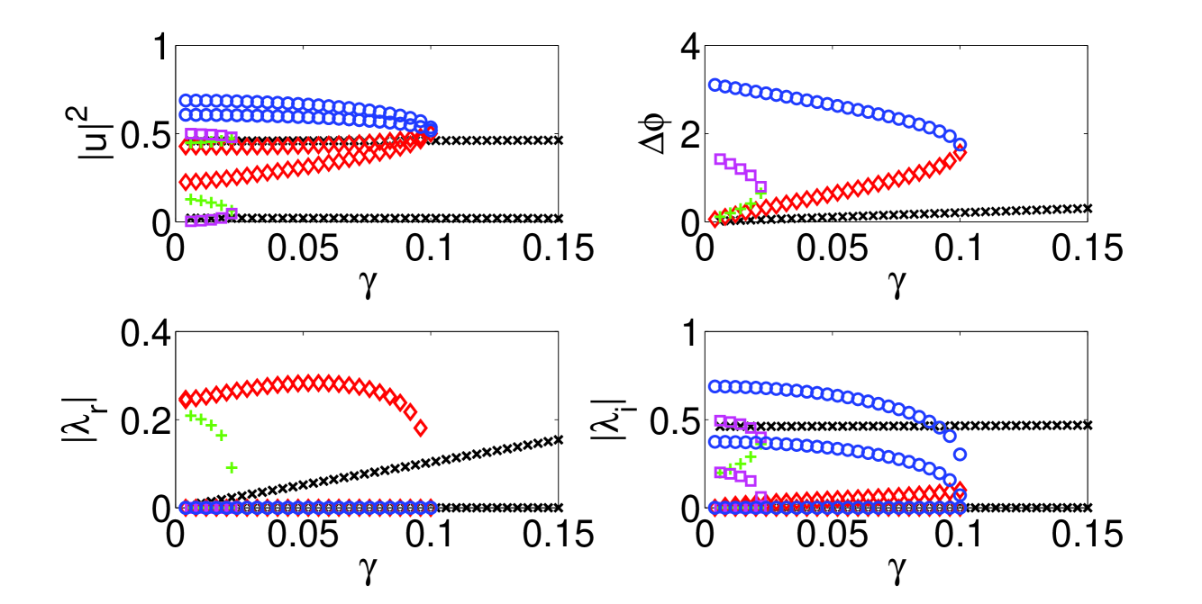
Figure 1: (Color online) The solution profile of Eq. (1) with $E=0.5$, $k=0.1$ and $\phi_{b}=0$. The four panels denote the solution amplitude (top left), phase differences between adjacent nodes (top right), real and imaginary parts (second row) of eigenvalues.

Since Eq. (4) is a polynomial of degree 5, we expect at most 5 distinct real roots (and at least 1 such). Indeed for suitable choices of the free parameters $(E,k)$, we identify five branches of stationary solutions. Figure 1 illustrates a situation with five branches under $E=0.5$ and $k=0.1$. Two of them, denoted by blue circles and red diamonds, collide and terminate at $\gamma=0.1$. The blue circles are essentially stable while the red diamonds are unstable. Another pair of branches, namely the magenta squares and green pluses collide and terminate at $\gamma=0.02$, with the magenta squares being stable and the green pluses being unstable (i.e., both of the above collisions are examples of saddle-center bifurcations). The black crosses branch, which is essentially unstable, persists beyond $\gamma=0.1$. Notice that the amplitudes of the different nodes for this branch shown in the top left panel of the figure are not constant: the upper line (standing for $B$) is slightly increasing and the lower line (standing for $A=C$) is slightly decreasing.

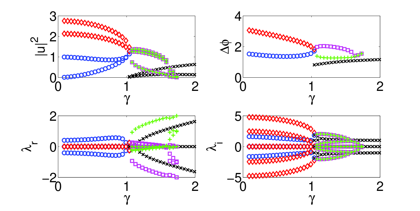
Figure 2: (Color online) In a way similar to that of the previous figure (i.e., with top left denoting amplitudes, top right relative phases, bottom left real and bottom right imaginary part of the linearization eigenvalues), the 4 panels show the existence and stability of solutions for a trimer with parameters $E=k=1$. There are three regular standing wave branches: the blue, the red and the black; the blue and red are the ones disappearing hand-in-hand at $\gamma=1.043$. Two ghost solutions are colored in magenta and green and bifurcate at the destabilization of the blue branch for $\gamma=1.035$, while they terminate for $\gamma=1.732$.

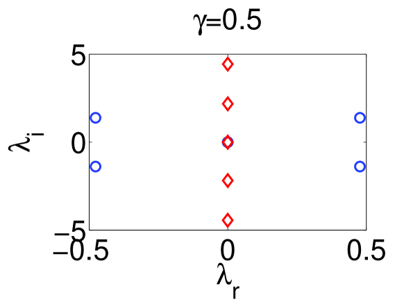
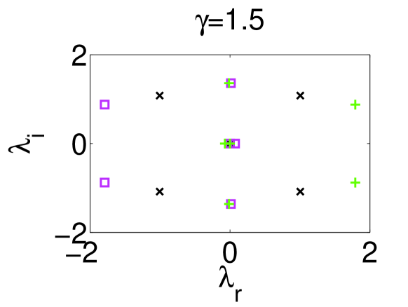
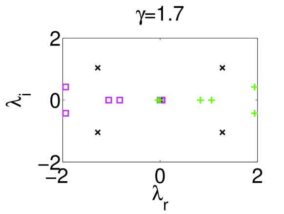
Figure 3: (Color online) The spectral planes $(\lambda_{r},\lambda_{i})$ of the eigenvalues $\lambda=\lambda_{r}+i\lambda_{i}$ of the solutions shown in Fig. 2. The first panel shows the case of $\gamma=0.5$ where only the standing wave branches exist (blue circles – unstable and red diamonds – stable). The second panel for $\gamma=1.5$ has only one standing wave (black crosses – unstable), and two asymmetric ghost states which are mirror images of each other (and so are their spectra), namely magenta squares and green pluses. The third panel shows the same branches as in top right but for $\gamma=1.7$ close to the termination of the ghost state branches.

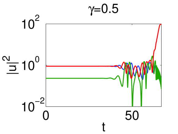
(a)  blue

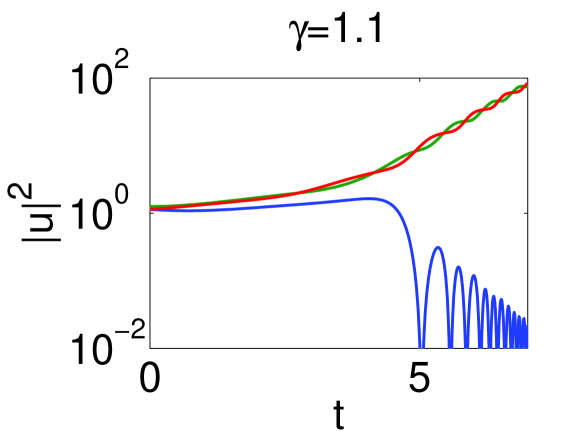
(b)  blue circles

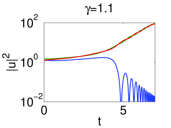
(c)  red diamonds

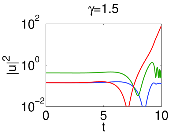
(d)  black crosses

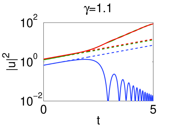
(e)  magenta squares

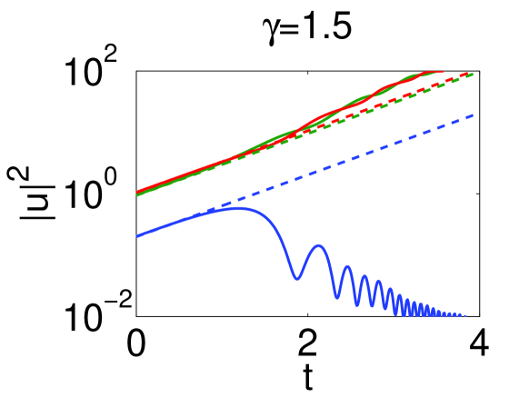
(f)  magenta squares

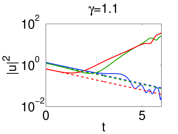
(g)  green pluses

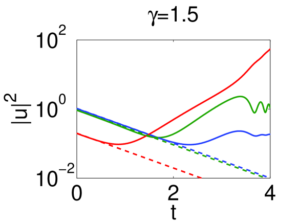
(h)  green pluses

Figure 4: (Color online) The dynamical evolution of the amplitudes of the three sites for the solutions shown in Fig. 2. Notice that all solutions are plotted in semilog. The first row shows the evolution of the three stationary branches. In (b) and (c), since these branches are absent for $\gamma=1.1$, their profile for $\gamma=1.043$ is initialized. The second row shows dynamics of the two ghost state solution branches. The dashed lines are the predicted dynamics of the ghost states on the basis of their growth (for magenta squares) or decay (for green pluses) rates.

In the following, we focus on a typical example of the branches (both stationary and ghost ones) for a selection of the free parameters of order unity, more specifically for $E=k=1$; cf. Fig. 2. We identify three distinct examples of stationary states denoted by the blue circle, red diamond and black cross branches. The blue circle and red diamond branches stem from the corresponding “+0–” and “–+–” branches, respectively, namely the second and third excited state of the Hamiltonian trimer problem of $\gamma=0$; cf. with Ref. todd . The blue circles branch is mostly unstable, except for a small interval of $\gamma\in[1,1.035]$, while the red diamonds branch is chiefly stable, except for the narrow interval of values of $\gamma\in[1.035,1.043]$. In this narrow interval, the eigenvalues of both of these branches are very close to each other. For the blue circles branch, we also note that two eigenvalue pairs stemming from a complex quartet collide on the imaginary axis at $\gamma=1$ and split as imaginary thereafter. One of these pairs exits as real for $\gamma>1.035$, and the two branches (blue circles and red diamonds) collide shortly thereafter, i.e., at $\gamma=1.043$.

On the other hand, Fig. 2 also reveals an additional branch, denoted by black crosses, that bifurcates from zero at $\gamma=1$ and persists for all values of $\gamma$ thereafter. This is quite interesting in its own right as an observation since, as highlighted in Ref. pgk , the linear critical point for the $\mathcal{P}\mathcal{T}$ phase transition is $\gamma=\sqrt{2}k$. Thus, this branch presents the simplest oligomer example (ones such are absent in the case of the dimer) whereby nonlinearity enables a solution family to persist past the point of the linear limit $\mathcal{P}\mathcal{T}$ phase transition. Additionally, it should be noted that the branch is stable for all values of $\gamma<1.13$, but destablizes for all larger values of $\gamma$.

In Fig. 2, however, in addition to the standard stationary solutions, the ghost state solutions are also shown. These are designated by the magenta squares and green pluses in the figure. These ghost solutions are also obtained for $\hat{E}=k=1$, and importantly (and contrary to what is the case for the stationary states), they bear distinct amplitudes in all three sites. The two (magenta and the green) branches shown in the figure are mirror images of each other, i.e., $A,B,C$ in the magenta branch are the same as $C,B,A$ in the green branch, respectively, and their phase difference and eigenvalues are opposite to each other. Notice that as indicated above the difference in the magnitudes of $A$ and $C$ supports the fact that these branches defy the expectations of the $\mathcal{P}\mathcal{T}$ symmetry. Indeed, both of the branches arise through a symmetry-breaking bifurcation from the blue branch when it becomes unstable at $\gamma=1.035$. Furthermore, it should be noted that the branches terminate at vanishing amplitude for $\gamma=1.732$. It is interesting to point out that when performing linear stability analysis of these states, we find both of them to be unstable. Case examples of the linearization results for both the regular states and the ghost ones are shown for three different values of $\gamma$ in Fig. 3. For $\gamma=0.5$, the red diamond branch is (marginally) stable, while the blue circle branch bears the instability that we discussed above for $\gamma<1$. For $\gamma=1.5$, only the black branch is present among the stationary ones and the magenta and green ghost state branches manifest their respective asymmetries with spectra that are asymmetric around the imaginary axis. This is a characteristic feature of the ghost states; see also R46 ; ricardo . Although among the two branches, the magenta is more stable and the green highly unstable, even the magenta branch is predicted to be weakly unstable with a small real positive eigenvalue. We will examine the dynamical implications of these instabilities in what follows. The last panel similarly shows the case of $\gamma=1.7$ shortly before the disappearance of the ghost state branches.

Finally, we examine the dynamics of the different branches in Fig. 4. The top row panels of the figure show the evolution of the three stationary branches. Panels (a) and (b) show the blue circle branch for $\gamma=0.5$ and $\gamma=1.1$, while panel (c) depicts the red diamond standing wave branch for $\gamma=1.1$. Notice that the cases of (b) and (c), the corresponding branches cease to exist at $\gamma=1.043$. Thus in these runs, we have used the terminal point profile of the branches (at $\gamma=1.043$) as initial data for the evolution with $\gamma=1.1$. Importantly, we note that in the unstable evolution of cases (b) and (c), two of the sites end up growing indefinitely while the lossy site ends up decaying. On the contrary, in the case (a), only the site with gain is led to growth, while the other two are led to eventual decay. In panel (d), we show the black crosses branch, the third among the standing wave solutions identified herein for $\gamma=1.5$. Notice that panel (d) shows a different dynamical evolution from panels (b) and (c) and more in line with panel (a), showcasing that there are indeed two general growth scenaria: one in which the gain site “grabs” along the neutral central site and leads it to indefinite growth and one in which the central site is ultimately led to decay together with the lossy site.

The four panels in the lower row show the dynamical evolution of the two ghost states (green pluses and magenta squares) for the cases of $\gamma=1.1$ and $\gamma=1.5$. With $E=E_{r}+iE_{i}$ being complex, the ghost state solutions under the form $u_{1}=\exp(iEt)a$, $u_{2}=\exp(iEt)b$ and $u_{3}=\exp(iEt)c$ should evolve exponentially, as indicated by dashed lines in panels (e)-(h). In particular, the magenta squares branch with negative $E_{i}$ is expected to lead to growth (for all three nodes of the trimer), while the green plus branch with positive $E_{i}$ is anticipated to decay (again for all nodes). The slopes of these growth/decay features are given by $-2E_{i}=-2\hat{E}\sin\phi_{e}$. However, in line with their anticipated linear “instability”, neither of these follows exactly the dynamics anticipated above. Both of them evolve for a short period according to the expected growth or decay, and then the gain sites start to grow and the loss sites start to decay, regardless of the trend predicted by the form of the ghost state (discussed above). Moreover, it is relevant to note as regards the corresponding dynamics that the cases of the blue circle and red diamond branches of $\gamma=1.1$ exhibit similar (asymptotic) dynamics to those of the magenta squares and of the green pluses for the same parameter value; i.e., the central site is also led to growth along with the gain one. On the other hand, it is also evident that the black crosses branch for $\gamma=1.5$ instead follow an evolution resembling to the asymptotic evolution of the green pluses branch (which is different from that of the magenta squares for the latter value). I.e., here only the gain site is ultimately led to growth.

Having unveiled the existence and stability, as well as nonlinear dynamical characteristics of the different solutions, we now turn to a discussion of the potential for experimental realization of $\mathcal{P}\mathcal{T}$-symmetry in optical systems especially as regards trimers, but also more generally.

IV Experimental realization of $\mathcal{P}\mathcal{T}$ optical systems

General requirements for realization of $\mathcal{P}\mathcal{T}$ optical systems are the availability of adequate methods for formation of coupled waveguide systems or arrays with the additional opportunity to spatially tailor loss and gain in the substrate. In other words, suitable fabrication conditions should allow for spatial manipulation of both real and imaginary part of the dielectric constant.

Laser crystals and glasses are amplifying media that may provide the necessary optical gain by using different physical mechanisms. Examples are doped bulk crystals and fibers that make use of stimulated emission to amplify a weak signal, electron-hole recombination in semiconductor optical amplifiers (SOAs), parametric amplification in nonlinear crystals, or stimulated Raman scattering (SRS). Furthermore, many laser gain materials allow for the formation of guiding index structures. However, although many amplifying materials exist, the most challenging aspect is the necessity to achieve optical gain while at the same time the real part of the refractive index should remain constant (or change only in a negligible way in order to maintain $\mathcal{P}\mathcal{T}$ symmetry), which is difficult to achieve because of the Kramers-Kronig relation. Besides thermo-optic effects in case of high optical powers, it turns out that other mechanisms like self-and cross-phase modulation are limiting the suitability of most laser gain media for application in $\mathcal{P}\mathcal{T}$ optics.

Another well-known amplification mechanism is optical beam coupling in photorefractive media like photovoltaic lithium niobate (LiNbO₃) crystals, which exists already at quite low optical light powers. Due to advanced waveguide formation techniques, LiNbO₃ is a favorite material for use in integrated optics Kip_APB1998 . Besides diffraction of weak signal beams on recorded index gratings which leads to gain, the point symmetry $3m$ of LiNbO₃ enables interaction of orthogonally polarized waves too Novikov1987 . A polarization grating recorded by a pump and signal beam having mutual orthogonal polarization allows for optical signal gain; the small-signal gain can reach several tens per cm for strong Fe doping Novikov1987 . At the same time, the spatially varying polarization pattern of pump and signal beam does not induce significant phase changes for the interacting beams. Using this mechanism, the first experimental demonstration of $\mathcal{P}\mathcal{T}$ symmetry in optics has been achieved in Fe:LiNbO₃ using Ti in-diffusion to form coupled waveguide structures R20 . However, there exist still some limitations that have to be overcome in order to realize more advanced $\mathcal{P}\mathcal{T}$ symmetric optical settings.

While spatial tailoring of optical gain may be achieved by limiting an optical pump beam to certain waveguide channels, this can be hardly done for loss (a technologically quite challenging solution consists in the formation of metallic stripes of precisely defined width on certain channels, see R18 ). Due to such difficulties, a more realistic experimental approach consists in allowing for a constant loss in all coupled channels, while this loss is overcompensated by adjustable gain in some selected channels only.

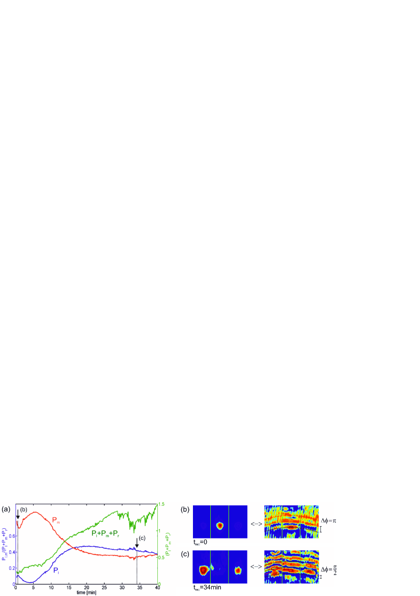
Figure 5: (Color online) (a) Evolution of powers in a three-channel coupler. Left and right channels experience equal gain; the lossy central channel is excited from the input facet. Gain develops due to holographic recording of a polarization grating according to $\gamma(t_{rec})=\gamma_{0}(1-\exp(-t_{rec}/\tau))$ with the photorefractive (Maxwell) time constant $\tau$. (b,c) Power distributions (left panel) on the end-facets for different recording times (b: $t_{rec}=0$; c: $t_{rec}=34$ min) and corresponding interferograms (right panels) showing the phase relation of central and outer channels.

An experimental example of a three-channel coupled waveguide structure having distributed gain and loss is shown in Fig. 5. While the precisely $\mathcal{P}\mathcal{T}$-symmetric pattern of loss-(neither gain nor loss)-gain is not directly realizable in the above described experiments, here we focus on a somewhat different configuration featuring an alternation of gain-loss-gain which is, arguably, the nearest experimentally realizable optical variant. To achieve that, three parallel single-mode waveguide channels for a wavelength of $\lambda=532\,$nm are formed on a Fe-doped x-cut LiNbO₃ substrate by in-diffusion of a stripe-like Ti film. The propagation length is 20 mm and the linear coupling coefficient is $k\approx 0.2\,$mm^-1. In the sample overall but constant loss is due to absorption of the used green light by in-diffused Fe ions. Similar to the arrangement in R20 , optical gain for the extraordinarily polarized signal is achieved by pumping the sample from the top using a plane wave of ordinary polarization. An amplitude mask on top of the substrate shields the central channel ($\sharp$2), thus (equal) gain is obtained for the left ($\sharp$1) and right ($\sharp$3) channels only. The signal light is coupled from the end-facet into the central channel. As can be seen, when the pump beam is switched on at time $t_{rec}=0$, power in the two outer channels start to increase. Simultaneously the total power (black symbols in Fig. 5) increases due to buildup of the polarization grating. Beside some asymmetries in the temporal evolution discussed below, for longer recording symmetry improves again, and the corresponding interferograms on the $rhs$ show the development of relative phase of central and outer channels, starting from the in-phase condition at $t_{rec}=0$ (Fig. 5b) towards a final phase difference of $\pm\pi/2$ at $t_{rec}\approx 34$ min (Fig. 5c). This relative phase development is in line with the earlier theoretical expectations on the basis of Eqns. such as (5)-(6). This behavior is also in good agreement with simulations of this gain-loss-gain system based on Runge-Kutta integration of the corresponding coupled-wave equations in Fig. 6. Of course, these runs also manifest the partial differences of this experimental realization from the genuinely $\mathcal{P}\mathcal{T}$-symmetric case in that ultimately all three waveguides feature growing optical power in the simulations of Fig. 6, a trait which is absent e.g. in Fig. 4 (where at least one waveguide is not growing indefinitely in power).

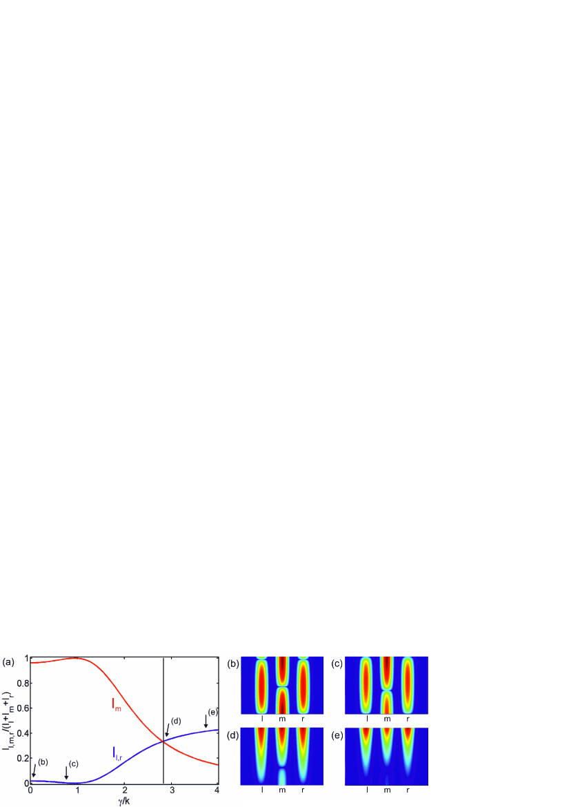
Figure 6: (Color online) (a) Simulation of normalized intensity of the three-channel coupler as a function of gain (normalized to $k$) using integration of the coupled-wave equations. The vertical line corresponds to $\gamma/k=2\sqrt{2}$, which is the “break even” point of this gain-loss-gain system. The four panels (b-e) on the right show the light power evolution during propagation for $\gamma/k=0$, (b), $\gamma/k=0.7$ (c), $\gamma/k=2.8$ (d), and $\gamma/k=3.7$ (e). For the false-color scale we choose a proportionality to $\sqrt[4]{I}$ to improve visibility of the amplified signal light in the channels.

Obviously, some experimental problems still exist. The temporal evolution in the left and right channels is far from being perfectly symmetric, especially for intermediate recording times. In most experiments, for long recording times (i.e. high gain) output powers of the three channels start to fluctuate slightly. Possible explanations for this behavior are large induced space-charge fields that may lead to spark plugs across the sample surface, or weak phase instabilities of the setup. A general problem is the small achievable gain, which is rarely sufficient to reach typical $\mathcal{P}\mathcal{T}$ symmetry-breaking thresholds in most of the fabricated samples. Gain is also limited because of low powers of signal and pump light: Higher signal power would lead to decoupling of the excited channel due to nonlinear index changes, while higher pump power would record a distorting phase gradient at the boundaries of the used amplitude mask (i.e. between illuminated/non-illuminated channels).

For future experiments using Fe:LiNbO₃ waveguide samples, a main objective will thus be to increase optical gain by optimizing material properties. However, when doping LiNbO₃ substrates with Fe using in-diffusion, the physical mechanisms that may lead to high gain when coupling orthogonally polarized waves are not yet fully understood: The influence of certain diffusion atmospheres, interference from simultaneous Ti in-diffusing used for waveguide formation, or the effect of Li out-diffusion at high temperatures and consequences on possible lattice sites of in-diffused Fe ions have not been investigated in detail. In particular, the high gain found in some Fe-doped bulk LiNbO₃ crystals has not been observed in waveguide samples so far.

An alternative experimental $\mathcal{P}\mathcal{T}$-symmetric model system that also uses LiNbO₃ with its well-developed waveguide fabrication technology as a substrate is Er doping to achieve gain in the optical communication window at $1.5\,\mu$m. Although no detailed data on cross-phase modulation when pumped e.g. with 980 nm wavelength is available yet, data from Er-doped fiber amplifiers (EDFAs) indicates that induced phase changes might be sufficiently small Jarabo1997 . Work on such systems is currently in progress, which may perhaps allow avoiding the described unwanted nonlinear effects that disturb the symmetry condition of the (real) refractive index in Fe-doped photorefractive LiNbO₃ for higher input powers.

V Conclusions & Future Challenges

In the present work, we have revisited the theme of one of the prototypical $\mathcal{P}\mathcal{T}$-symmetric oligomers, namely the trimer. We have illustrated the different number of branches (at least one and at most five) of standing wave solutions that exist for this system. We have thereafter focused on a case example of parameters of order unity and have shown that two of these standing wave branches terminate in a pairwise disappearance, while the third one exists for values of the gain/loss parameter, in fact, extending past the point of the $\mathcal{P}\mathcal{T}$-symmetry breaking phase transition of the linear limit occuring at $\gamma=\sqrt{2}k$.

Additionally, we have also presented the formulation of the so-called ghost states in this system and have explicitly computed them, showing how they emerge through a symmetry breaking bifurcation (asymmetrizing the amplitudes of the two side sites $A$ and $C$) from one of the standing wave branches. As expected on the basis of such an effective pitchfork bifurcation, the two resulting ghost state branches are mirror-images of each other (and so are their corresponding spectra). The dynamics of both the unstable stationary states and those of the ghost states revealed two possible dynamical scenaria. In one of these, the “neutral” site (without gain or less) sided with the gain one, while the other corresponded to the case where it sided with the lossy site.

Additionally, we have explored the possibility of creating $\mathcal{P}\mathcal{T}$ symmetric systems in nonlinear optics, revealing that it is arguably simpler to create e.g. a gain-loss-gain three-channel system, rather than the genuinely $\mathcal{P}\mathcal{T}$ symmetric situation where a waveguide with gain and one with loss straddle a middle one without either gain or loss. On the other hand, for this gain-loss-gain setting, we presented both physical experiments and corroborating numerical simulations revealing the partition of the fraction of optical power (initially placed at the central channel) and how it transfers more to the outer gain channels as the gain is increased beyond $\gamma/k=1$.

There are many interesting questions that arise from the present study and are worthy of further exploration. It would be interesting to generalize our considerations herein to the case of quadrimers and to appreciate how the complexity of the relevant configurations expands, especially since in the latter case, there is generally the potential of two gain/loss parameters konozezy ; nevertheless per the above discussion on experimental possibilities in optics, the case of two waveguides with equal gain and two with equal loss would appear as the most realistic one presently. At the same time, further experimental implementations of oligomer systems, either at the electrical circuit level, or at the optical waveguide level discussed in the last section would be particularly desirable and highly interesting towards an increased understanding of the systems’ dynamics. Efforts in these directions are currently in progress and will be reported in future publications.

- (1) C. M. Bender and S. Boettcher, Phys. Rev. Lett. 80, 5243 (1998); C. M. Bender, S. Boettcher and P. N. Meisinger, J. Math. Phys. 40, 2201 (1999).
- (2) C. M. Bender, Rep. Prog. Phys. 70, 947 (2007).
- (3) A. Ruschhaupt, F. Delgado, and J. G. Muga, J. Phys. A: Math. Gen. 38, L171 (2005).
- (4) A. Guo, G. J. Salamo, D. Duchesne, R. Morandotti, M. Volatier-Ravat, V. Aimez, G. A. Siviloglou, and D. N. Christodoulides, Phys. Rev. Lett. 103, 093902 (2009).
- (5) C. E. Rüter, K. G. Makris, R. El-Ganainy, D. N. Christodoulides, M. Segev, and D. Kip, Nature Phys. 6, 192 (2010).
- (6) A. Regensburger, C. Bersch, M.-A. Miri, G. Onishchukov, D. N. Christodoulides, and U. Peschel, Nature 488, 167 (2012).
- (7) J. Schindler, A. Li, M. C. Zheng, F. M. Ellis, and T. Kottos, Phys. Rev. A 84, 040101 (2011).
- (8) H. Ramezani, T. Kottos, R. El-Ganainy, and D. N. Christodoulides, Phys. Rev. A 82, 043803 (2010).
- (9) M. C. Zheng, D. N. Christodoulides, R. Fleischmann, and T. Kottos, Phys. Rev. A 82, 010103(R) (2010).
- (10) K. Li and P. G. Kevrekidis, Phys. Rev. E 83, 066608 (2011).
- (11) A. A. Sukhorukov, Z. Xu, and Yu. S. Kivshar, Phys. Rev. A 82, 043818 (2010).
- (12) F. Kh. Abdullaev, V.V. Konotop, M. Ögren, and M. P. Sørensen, Opt. Lett. 36, 4566 (2011).
- (13) R. Driben and B. A. Malomed, Opt. Lett. 36, 4323 (2011).
- (14) R. Driben and B. A. Malomed, Europhys. Lett. 96, 51001 (2011).
- (15) I. V. Barashenkov, S. V. Suchkov, A. A. Sukhorukov, S. V. Dmitriev, and Yu. S. Kivshar, Phys. Rev. A 86, 053809 (2012).
- (16) N. V. Alexeeva, I. V. Barashenkov, A. A. Sukhorukov, and Yu. S. Kivshar, Phys. Rev. A 85, 063837 (2012).
- (17) V. Achilleos, P. G. Kevrekidis, D. J. Frantzeskakis, and R. Carretero-González Phys. Rev. A 86, 013808 (2012).
- (18) D. A. Zezyulin and V. V. Konotop, Phys. Rev. A 85, 043840 (2012); Yu. V. Bludov, V. V. Konotop, and B. A. Malomed, Phys. Rev. A 87, 013816 (2013).
- (19) H. Cartarius and G. Wunner, Phys. Rev. A 86, 013612 (2012); H. Cartarius, D. Haag, D. Dast, and G. Wunner, J. Phys. A 45, 444008 (2012).
- (20) E.-M. Graefe, J. Phys. A 45, 444015 (2012).
- (21) A. S. Rodrigues, K. Li, V. Achilleos, P. G. Kevrekidis, D. J. Frantzeskakis, C. M. Bender, Rom. Rep. Phys. 65, 5 (2013).
- (22) D. Leykam, V. V. Konotop, and A. S. Desyatnikov, Opt. Lett. 38, 371 (2013).
- (23) K. Li, P. G. Kevrekidis, B. A. Malomed, and U. Günther, J. Phys. A: Math. Theor. 45, 444021 (2012).
- (24) V. Achilleos, P. G. Kevrekidis, D. J. Frantzeskakis, R. Carretero-González, arXiv:1208.2445.
- (25) M. Duanmu, K. Li, R. L. Horne, P. G. Kevrekidis and N. Whitaker, Phil. Trans. Roy. Soc. A 371, 20120171 (2013).
- (26) D. A. Zezyulin and V. V. Konotop Phys. Rev. Lett. 108, 213906 (2012).
- (27) T. Kapitula, P. G. Kevrekidis and Z. Chen, SIAM J. Appl. Dyn. Sys. 5, 598 (2006).
- (28) D. Kip, Appl. Phys. B: Laser and Optics 67, 131 (1998).
- (29) A. Novikov, S. Odoulov, O. Oleinik, and B. Sturman, Ferroelectrics 75, 295 (1987).
- (30) S. Jarabo, J. Opt. Soc. Am. B 14, 1846 (1997).