Breakdown of Kohn Theorem Near Feshbach Resonance

Abstract

We study the collective excitation frequencies of a harmonically trapped ⁸⁵Rb Bose-Einstein condensate (BEC) in the vicinity of a Feshbach resonance. To this end, we solve the underlying Gross-Pitaevskii (GP) equation by using a Gaussian variational approach and obtain the coupled set of ordinary differential equations for the widths and the center of mass of the condensate. A linearization shows that the dipole mode frequency decreases when the bias magnetic field approaches the Feshbach resonance, so the Kohn theorem is violated.

I Introduction

Many experiments focus on investigating collective excitations of harmonically trapped BECs as they can be measured very accurately and, therefore, allow for extracting the respective system parameters StamperKurn . Several studies show that the excitation of low-lying collective modes can be achieved by modulating a system parameter. One example is to change periodically the external potential trap DSJin ; MOMewes ; YCastinandRDum ; FDalfovo ; JJGarciaRipoll ; JJGarciaRipoll1 ; AINicolin or, more specifically, the trap anisotropy of the confining potential FDalfovo ; GHechenblaikner1 ; hodby ; YuZhou ; Hamid1 ; Hamid2 . Alternatively, this can also be achieved by a periodic modulation of the s-wave scattering length VSBagnato0 ; SEPollackandRGHulet ; VSBagnato ; IVidanovic ; SSabari ; AINicolin1 ; will or, possibly, by modifying the three-body interaction strength SSabari ; Hamid1 ; Hamid2 .

In 1961 W. Kohn kohn showed in a three-dimensional solid that the Coulomb interaction between electrons does not change the cyclotron resonance frequency. This Kohn theorem can also be transfereed to the realm of ultracold quantum gases, where it states that the center of mass of the entire cloud oscillates back and forth in the harmonic trapping potential with the natural frequency of the trap irrespective of both the strength and type of the two-body interaction. The Kohn theorem for a Bose gas is discussed explicitly in the Bogoliubov approximation at zero temperature of Ref. DanielRokhsar . The dynamics of a trapped Bose condensed gas at finite temperature are consistent with a generalized Kohn theorem and satisfy the linearized ZNG hydrodynamic equations in Ref. Zaremba2771999 . In particular, the Kohn mode was studied in an approximate variational approach to the kinetic theory in the collisionless regime in Ref. STOOFkohn . The validity of the Kohn theorem at finite temperature was also shown within a linear response treatment in Ref. Minguzzi . Later on it was also examined in Ref. Jurgen for a specific finite-temperature approximation within the dielectric formalism. Furthermore, the dipole mode frequency was studied by using a sum rule approach in Refs. sum1 ; sum11 ; sum2 ; sum3 ; sum4 . The collective dipole oscillations in the Bose-Fermi mixture were studied theoretically in Refs. sum11 ; sum2 and experimentally in Ref. sum5 , while the dipole oscillation of a spin-orbit coupled Bose-Einstein condensate confined in a harmonic trap was studied experimentally sum3 and investigated theoretically sum3 ; sum4 . The dipole oscillation was also discussed for a general fermionic mixture by using the Boltzmann equation in Ref. sum6 .

Apart from a periodic modulation of a system parameter the dipole mode can also be excited by introducing an abrupt change in the potential. The experimental achievement StamperKurn ; YANGLu has been confirmed by Refs. CJPethick ; SStringari , where also the quadrupole frequency was determined as an eigenfrequency of the hydrodynamic equations. The coupling between the internal and the external dynamics of a Bose-Einstein condensate oscillating in an anharmonic magnetic waveguide was studied in Ref. HOtt . There also several nonlinear effects including second and third harmonic generation of the center of mass motion, and a nonlinear mode mixing have been identified. In the more recent work Bagnato12 , the authors explored a different physical idea by investigating the coupling between dipole and quadrupole modes in the immediate vicinity of a Feshbach resonance. They started with considering a Bose-Einstein condensate in a magneto-optical Ioffe-Pritchard trap Ioffe with a controlled bias field, where the dipole mode is excited. If the bias field is close enough to a Feshbach resonance, the oscillation of the entire cloud through the inhomogeneous bottom of the trap causes an effective periodic time-dependent modulation in the scattering length, which in turn changes the Kohn mode frequency, but also excites other modes like the quadrupole or the breathing mode.

Although Ref. Bagnato12 introduces this appealing physical notion, it only provides a rough quantitative study. Therefore we calculate in this paper in detail the collective excitation modes of a harmonically trapped Bose-Einstein condensate in the vicinity of a Feshbach resonance for experimentally realistic parameters of a ⁸⁵Rb BEC RB85 ; RB85Grimm . To this end, we consider the situation that a Bose-Einstein condensate oscillates within a dipole mode in $z$-direction and investigate how the dipole mode frequency changes when the bias magnetic field approaches the Feshbach resonance in Section II. Afterwards, we follow Ref. Bagnato12 and transform the partial differential of GP equation Grosseq ; Pitaevskiieq for the condensate wave function in Section III within a variational approach Perezandzoller ; VMPerez into a set of ordinary differential equations for the widths and the center of mass position of the condensate in an axially-symmetric harmonic trap plus a bias potential. Our analysis is based on an exact treatment with the help of the Schwinger trick schwinger . The resulting theory on how to determine the low-lying collective excitation frequencies is developed step by step in Section IV. Afterwards, Section V compares our results with the corresponding findings of Ref. Bagnato12 . In addition we discuss two special cases, when the bias magnetic field field approaches the Feshbach resonance and when it is far away from the Feshbach resonance. It turns out that the heuristic approximation in Ref. Bagnato12 is not valid neither on top of the Feshbach resonance, nor far away from it. Finally, in Sec. VI we summarize our findings and present the conclusions.

II Near Feshbach Resonance

The dynamics of a condensed Bose gas in a trap at zero temperature is described by the time-dependent GP equation Perezandzoller ; VMPerez

$$i\hbar\frac{\partial\psi({\bf r},t)}{\partial t}=\Bigg{[}-\frac{\hbar^{2}}{2M}\Delta+V_{\rm{ext.}}({\bf r})+g_{2}Nn_{c}({\bf r},t)\Bigg{]}\psi({\bf r},t).$$ (1)

where $\psi({\bf r},t)$ denotes a condensate wave function and $N$ represents to the total number of atoms in the condensate. On the right-hand side of the above equation we have a kinetic energy term, where $M$ denotes the mass of the corresponding atomic species, an external trap $V_{\rm{ext.}}({\bf r})$, and the third is the two-body interaction with the condensate density $n_{c}({\bf r},t)=\left|\psi({\bf r},t)\right|^{2}$ and the strength $g_{2}=4\pi\hbar^{2}a_{\rm s}/M$, which is proportional to the $s$-wave scattering length $a_{\rm s}$. In the presence of a magnetic field, the s-wave scattering length can be tuned by applying an external magnetic field due to the Feshbach resonance CJPethick ; Moerdijk

$$a_{s}(B)=a_{\rm{BG}}\bigg{(}1-\frac{\Delta}{B-B_{\rm{res}}}\bigg{)}\,,$$ (2)

with the background s-wave scattering $a_{\rm{BG}}$, the width of the Feshbach resonance $\Delta$, and the resonance of magnetic field $B_{\rm{res}}$. In this paper, we consider a Bose-Einstein condensate confined in a magneto-optical Ioffe-Pritchard trap composed of a cylindrically symmetric harmonic potential with trap anisotropy $\lambda$ plus a bias Bagnato12 ; Ioffe :

$$V_{\rm{ext.}}({\bf r})=V_{0}+\frac{M\omega^{2}_{\rho}}{2}\left(\rho^{2}+\lambda^{2}z^{2}\right).$$ (3)

Due to the atomic magnetic moment $\mu_{\rm B}$ the potential is generated by a corresponding magnetic field whose modulus is given by

$$B=B_{0}+\frac{M\omega^{2}_{\rho}}{2\mu_{\rm B}}\left(\rho^{2}+\lambda^{2}z^{2}\right)\,,$$ (4)

where $B_{0}=V_{0}/\mu_{\rm B}$ is the bias field.

From Eqs. (2) and (4), the inter-particle interaction in the atomic cloud moving in this potential is controlled by the spatially dependent scattering length

$$a_{\rm s}=a_{\rm{BG}}\bigg{[}1-\frac{\Delta}{\mathcal{H}+\frac{M\omega^{2}_{\rho}}{2\mu_{\rm B}}\left(\rho^{2}+\lambda^{2}z^{2}\right)}\bigg{]}\,,$$ (5)

where $\mathcal{H}=B_{0}-B_{\rm{res}}$ denotes the deviation of the bias magnetic field $B_{0}$ from the location of the Feshbach resonance at $B_{\rm res}$. In the following, we consider the potential (3) loaded with a condensed cloud whose dipole mode is excited in the $z$-direction. In this configuration, far away from the Feshbach resonance the center of mass oscillates periodically at the bottom of the trap with the Kohn mode frequency $\omega_{z}=\lambda\omega_{\rho}$.

As an initial physical motivation we discuss the consequences of the Thomas-Fermi (TF) approximation. As we assume to have a strong two-body interaction, we neglect the kinetic energy term in the time-independent counterpart of Eq. (1) and obtain

$$\mu=V_{\rm{ext.}}({\bf r})+g_{2}n_{c}({\bf r}).$$ (6)

Far away from the Feshbach resonance we can consider the potential contribution in Eq. (5) to be small, thus we expand Eq. (5) up to the first order of the external potential, yielding

$$\mu=V_{\rm{ext.}}({\bf r}) +\frac{4\pi\hbar^{2}a_{\rm{BG}}n_{c}({\bf 0})}{M}\bigg{[}1-\frac{\Delta}{\mathcal{H}}$$

$$+\frac{\Delta M\omega^{2}_{\rho}}{2\mathcal{H}^{2}\mu_{\rm B}}\left(\rho^{2}+\lambda^{2}z^{2}\right)+.....\bigg{]}\,,$$ (7)

where $n_{c}({\bf 0})$ is the TF density at the trap center with the chemical potential $\mu=\frac{\hbar\omega_{\rho}}{2}\left(\frac{15N\lambda a_{\rm eff}}{l}\right)^{2/5}$. On the one hand we read off from Eq. (7) an effective s-wave scattering length

$$a_{\rm eff}=a_{\rm BG}\left(1-\frac{\Delta}{\mathcal{H}}\right)\,.$$ (8)

In the following discussion we have a ⁸⁵Rb BEC in mind, whose Feshbach resonance is characterized by a negative background value of the s-wave scattering length, i.e. $a_{\rm{BG}}<0$, and a positive width, i.e. $\Delta>0$ RB85 ; RB85Grimm . Thus, the BEC is unstable, i.e. $a_{\rm eff}<0$, provided that $B_{0}<B_{\rm crit}+\Delta$. Conversely, the TF approximation yields a stable BEC, i.e. $a_{\rm eff}>0$, in the case that $B_{\rm res}<B_{0}<B_{\rm crit}=B_{\rm res}+\Delta$. On the other hand, we obtain from Eqs. (3) and (7) an effective Kohn mode frequency

$$\omega_{D,\rm{eff}}=\lambda\omega_{\rho}\sqrt{1+\frac{4\pi\hbar^{2}a_{\rm{BG}}n_{c}({\bf 0})\mu\Delta}{M\mathcal{H}^{2}\mu_{\rm B}}}\,.$$ (9)

Thus, on the right-hand side of the Feshbach resonance, i.e. for $B_{\rm res}<B_{0}<B_{\rm crit}=B_{\rm res}+\Delta$, we expect due to $a_{\rm BG}<0$ that the Kohn mode frequency Eq. (9) is smaller than the corresponding one without the Feshbach resonance. In the following we will show that this initial qualitative finding is confirmed by a more quantitative analysis. In particular, it will turn out that the leading change of the Kohn mode frequency far away from the Feshbach resonance is, indeed, of the order $1/\mathcal{H}^{2}$.

III Variational Approach

Equation (1) can be cast into a variational problem, which corresponds to the extremization of the action defined by the Lagrangian

$$L(t) = \int d{\bf r}\bigg{[}\frac{i\hbar}{2}\left(\psi^{*}\frac{\partial\psi}{\partial t}-\psi\frac{\partial\psi^{*}}{\partial t}\right)$$ (10)

$$-\ \ \frac{\hbar^{2}}{2M}|\nabla\psi|^{2}-V({\bf r})|\psi|^{2}-\frac{g_{2}N}{2}|\psi|^{4}\,\bigg{]}.$$

In order to analytically study the dynamical system of a BEC with two-body contact interaction, where the dipole mode is excited in $z$-direction, we use a Gaussian variational ansatz which includes the center of mass oscillation in the $z$-direction according to Refs. Perezandzoller ; VMPerez ; Bagnato12 . For an axially symmetric trap, this time-dependent ansatz reads

$$\psi^{G}(\rho,z,t) = {\mathcal{N}}(t)\exp\bigg{[}-\frac{\rho^{2}}{2u_{\rho}^{2}}+i\rho\alpha_{\rho}+i\rho^{2}\beta_{\rho}\bigg{]}$$ (11)

$$\times\exp\bigg{[}-\frac{(z-z_{0})^{2}}{2u_{z}^{2}}+iz\alpha_{z}+iz^{2}\beta_{z}\bigg{]},$$

where $\mathcal{N}=1/\sqrt{\pi^{\frac{3}{2}}u_{\rho}^{2}u_{z}}$ is a normalization factor, while $u_{\rho,z}$, $z_{0}$, $\alpha_{\rho,z}$, and $\beta_{\rho,z}$ denote time-dependent variational parameters, which represent radial and axial condensate widths, the center of mass position, and the corresponding phases. Inserting the Gaussian ansatz (11) into the Lagrange function (10), we obtain

$$L(t)=-\frac{\hbar^{2}}{2M}\bigg{[}\frac{1}{2u_{z}^{2}}+\frac{1}{u_{\rho}^{2}}+2u_{z}^{2}\beta_{z}^{2}+4z_{0}^{2}\beta_{z}^{2}+4z_{0}\beta_{z}\alpha_{z}$$

$$+\alpha_{z}^{2}+4u_{\rho}^{2}\beta_{\rho}^{2}+2\sqrt{\pi}u_{\rho}\beta_{\rho}\alpha_{\rho}+\alpha_{\rho}^{2}\bigg{]}-\frac{\hbar}{2}\bigg{[}u_{z}^{2}\dot{\beta}_{z}+2z_{0}^{2}\dot{\beta}_{z}$$

$$+2z_{0}\dot{\alpha}_{z}+2u_{\rho}^{2}\dot{\beta}_{\rho}+\sqrt{\pi}u_{\rho}\dot{\alpha}_{\rho}\bigg{]}-V_{0}-\frac{\hbar^{2}Na_{\rm{BG}}}{\sqrt{2\pi}M}\frac{1}{u^{2}_{\rho}u_{z}}$$

$$-\frac{M\omega^{2}_{\rho}}{2}\bigg{[}u^{2}_{\rho}+\frac{\lambda^{2}u^{2}_{z}}{2}+\lambda^{2}z_{0}^{2}\bigg{]}+\frac{4\hbar^{2}Na_{\rm{BG}}\Delta}{\pi u^{4}_{\rho}u_{z}^{2}M}f\,,$$ (12)

where we have introduced the integral

$$f=\int_{0}^{\infty}d\rho\int_{-\infty}^{\infty}dz\frac{\rho\exp\bigg{[}-2\rho^{2}/u_{\rho}^{2}-2(z-z_{0})^{2}/u_{z}^{2}\bigg{]}}{\mathcal{H}+\frac{M\omega^{2}_{\rho}}{2\mu_{\rm B}}\left(\rho^{2}+\lambda^{2}z^{2}\right)}.$$ (13)

From the corresponding Euler-Lagrange equations we obtain the equations of motion for all variational parameters. The phases $\alpha_{\rho,z}$ and $\beta_{\rho,z}$ can be expressed explicitly in terms of first derivatives of the widths $u_{\rho}$, $u_{z}$, and the center of mass coordinate $z_{0}$ according to

$$\alpha_{\rho} =0\,,\hskip 9.95863pt\alpha_{z}=\frac{M}{\hbar}\dot{z}_{0}-2z_{0}\beta_{z}\,,\hskip 9.95863pt\beta_{\rho,z}=\frac{M}{2\hbar}\frac{\dot{u}_{\rho,z}}{u_{\rho,z}}\,.$$ (14)

Inserting Eq. (14) into the Euler-Lagrange equations for the width of the condensates $u_{\rho}$, $u_{z}$, and the center of mass coordinate $z_{0}$, we obtain a system of three second-order differential equations for $u_{\rho}$, $u_{z}$, and $z_{0}$: After rescaling the quantities according to

$$u_{i},\rho,z,z_{0}\rightarrow l(u_{i},\rho,z,z_{0}),\ \ t\rightarrow t\omega_{\rho}\,,$$ (15)

with the oscillating length $l=\sqrt{\hbar/(M\omega_{\rho})}$, we obtain a system of second-order differential equations for $u_{\rho}$, $u_{z}$, and $z_{0}$ in the dimensionless form Bagnato12

$$\ddot{u}_{\rho}+u_{\rho}-\frac{1}{u_{\rho}^{3}}-\frac{\mathcal{P}_{\rm{BG}}}{u_{z}u_{\rho}^{3}}$$ (16)

$$\hskip 14.22636pt\times\bigg{[}1-\frac{16\varepsilon_{0}f}{\sqrt{2\pi}l^{3}u_{\rho}^{2}u_{z}}+\frac{4\varepsilon_{0}}{\sqrt{2\pi}l^{2}u_{\rho}u_{z}}\frac{\partial f}{\partial u_{\rho}}\bigg{]}=0\,,$$

$$\ddot{u}_{z}+\lambda^{2}u_{z}-\frac{1}{u_{z}^{3}}-\frac{\mathcal{P}_{\rm{BG}}}{u_{z}^{2}u_{\rho}^{2}}$$ (17)

$$\hskip 14.22636pt\times\bigg{[}1-\frac{16\varepsilon_{0}f}{\sqrt{2\pi}l^{3}u_{\rho}^{2}u_{z}}+\frac{8\varepsilon_{0}}{\sqrt{2\pi}l^{2}u_{\rho}^{2}}\frac{\partial f}{\partial u_{z}}\bigg{]}=0\,,$$

$$\ddot{z}_{0}+\lambda^{2}z_{0}-\frac{4\mathcal{P}_{\rm{BG}}\varepsilon_{0}}{\sqrt{2\pi}l^{2}u^{4}_{\rho}u_{z}^{2}}\frac{\partial f}{\partial z_{0}}=0\,.$$ (18)

Here we have introduced the dimensionless parameters

$$\mathcal{P}_{\rm{BG}}=\sqrt{\frac{2}{\pi}}\frac{Na_{\rm{BG}}}{l},\,\varepsilon_{0}=\frac{\Delta}{\mathcal{H}},\,\varepsilon_{1}=\frac{\mathcal{H}\mu_{\rm B}}{(\hbar\omega_{\rho})},\,\varepsilon=\varepsilon_{0}\,\varepsilon_{1}\,.$$ (19)

In order to study the frequencies of collective modes both in the vicinity of the Feshbach resonance and on the right-hand side of the Feshbach resonance, i.e. for $\mathcal{H}>0$, we develop now our own approach by using the Schwinger trick schwinger in order to rewrite the integral Eq. (13) in form of

$$f =l^{3}\int_{0}^{\infty}d\rho\int_{-\infty}^{\infty}dz\int_{0}^{\infty}d\mathcal{S}\ \rho\exp\bigg{[}-\frac{2\rho^{2}}{u_{\rho}^{2}}-\frac{2(z-z_{0})^{2}}{u_{z}^{2}}\bigg{]}$$

$$\hskip 11.38092pt\times\exp\bigg{[}-\mathcal{S}-\frac{\mathcal{S}}{2\varepsilon_{1}}\left(\rho^{2}+\lambda^{2}z^{2}\right)\bigg{]}\,.$$ (20)

In the following, we concentrate on the topic how this violates the Kohn theorem, i.e. how the dipole mode frequency changes when the bias magnetic field $B_{0}$ approaches the Feshbach resonance $B_{\rm res}$. Within the linearization of the equations of motions (16)–(18), we have to take into the account that the equilibrium value of the center of mass position vanishes according to Eq. (18). This allows to expand the integral of Eq. (20) up to the second order of $z_{0}$, which yields

$$f = l^{3}\int_{0}^{\infty}d\rho\int_{-\infty}^{\infty}dz\int_{0}^{\infty}d\mathcal{S}\ \rho\bigg{[}1+\frac{4zz_{0}}{u_{z}^{2}}-\frac{2z_{0}^{2}}{u_{z}^{2}}+\frac{8z^{2}z_{0}^{2}}{u_{z}^{4}}+..\bigg{]}$$ (21)

$$\times\exp\left[-\frac{2\rho^{2}}{u_{\rho}^{2}}-\frac{2z^{2}}{u_{z}^{2}}-\mathcal{S}-\frac{\mathcal{S}}{2\varepsilon_{1}}\left(\rho^{2}+\lambda^{2}z^{2}\right)\right]\,.$$

Correspondingly we determine the respective first derivatives $\frac{\partial f}{\partial u_{\rho}}$, $\frac{\partial f}{\partial u_{z}}$, and $\frac{\partial f}{\partial z_{0}}$ which appear in the equations of motion (16)–(18).

IV Right-Hand Side of Feshbach Resonance

We consider in this section the frequencies of collective modes when the bias field $B_{0}$ is larger than or equal to the resonant magnetic field $B_{\rm{res}}$, i.e. $\mathcal{H}=B_{0}-B_{\rm{res}}\geq 0$.

IV.1 Collective Mode Frequencies

At first we obtain a system of three second-order ordinary differential equations for $u_{\rho}$, $u_{z}$, and $z_{0}$ in the dimensionless form after inserting Eq. (21) into Eqs. (16)–(18):

$$\ddot{u}_{\rho}+ u_{\rho}-\frac{1}{u_{\rho}^{3}}-\frac{\mathcal{P}_{\rm{BG}}}{u_{z}u_{\rho}^{3}}$$

$$\times\bigg{[}1-16\int_{0}^{\infty}\frac{\varepsilon\ \varepsilon_{1}^{1/2}d\mathcal{S}\ e^{-\mathcal{S}}\left(2\varepsilon_{1}+\mathcal{S}u_{\rho}^{2}\right)}{\left(4\varepsilon_{1}+\mathcal{S}u_{\rho}^{2}\right)^{2}\sqrt{4\varepsilon_{1}+\mathcal{S}u_{z}^{2}\lambda^{2}}}+...\bigg{]}=0,$$

$$\ddot{u}_{z}+ \lambda^{2}u_{z}-\frac{1}{u_{z}^{3}}-\frac{\mathcal{P}_{\rm{BG}}}{u_{z}^{2}u_{\rho}^{2}}$$

$$\times\bigg{[}1-16\int_{0}^{\infty}\frac{\varepsilon\ \varepsilon_{1}^{1/2}d\mathcal{S}\ e^{-\mathcal{S}}\left(2\varepsilon_{1}+\mathcal{S}u_{z}^{2}\lambda^{2}\right)}{\left(4\varepsilon_{1}+\mathcal{S}u_{\rho}^{2}\right)\left(4\varepsilon_{1}+\mathcal{S}u_{z}^{2}\lambda^{2}\right)^{3/2}}+...\bigg{]}=0,$$

$$\ddot{z}_{0}+ \lambda^{2}z_{0}\bigg{[}1+\frac{16\mathcal{P}_{\rm{BG}}}{u^{2}_{\rho}u_{z}}$$

$$\times\int_{0}^{\infty}\frac{\varepsilon\ \varepsilon_{1}^{1/2}d\mathcal{S}\ e^{-\mathcal{S}}\mathcal{S}}{\left(4\varepsilon_{1}+\mathcal{S}u_{\rho}^{2}\right)\left(4\varepsilon_{1}+\mathcal{S}u_{z}^{2}\lambda^{2}\right)^{3/2}}+...\bigg{]}=0\,\,.$$

The time-independent solution of the condensate widths $u_{\rho}=u_{\rho 0}$, $u_{z}=u_{z0}$, and $z_{0}=z_{00}$ is determined from

$$u_{\rho 0}-\frac{1}{u_{\rho 0}^{3}}-\frac{\mathcal{P}_{\rm{BG}}}{u_{z0}u_{\rho 0}^{3}}\bigg{[}1-16\varepsilon\ \varepsilon_{1}^{1/2}$$

$$\times\int_{0}^{\infty}\frac{d\mathcal{S}\ e^{-\mathcal{S}}\left(2\varepsilon_{1}+\mathcal{S}u_{\rho 0}^{2}\right)}{\left(4\varepsilon_{1}+\mathcal{S}u_{\rho 0}^{2}\right)^{2}\sqrt{4\varepsilon_{1}+\mathcal{S}u_{z0}^{2}\lambda^{2}}}\bigg{]}=0\,,$$ (25)

$$\lambda^{2}u_{z0}-\frac{1}{u_{z0}^{3}}-\frac{\mathcal{P}_{\rm BG}}{u_{z0}^{2}u_{\rho 0}^{2}}\bigg{[}1-16\varepsilon\ \varepsilon_{1}^{1/2}$$

$$\times\int_{0}^{\infty}\frac{d\mathcal{S}\ e^{-\mathcal{S}}\left(2\varepsilon_{1}+\mathcal{S}u_{z0}^{2}\lambda^{2}\right)}{\left(4\varepsilon_{1}+\mathcal{S}u_{\rho 0}^{2}\right)\left(4\varepsilon_{1}+\mathcal{S}u_{z0}^{2}\lambda^{2}\right)^{3/2}}\bigg{]}=0,$$ (26)

$$z_{00}=0\,\,.$$ (27)

Using the Gaussian approximation enables us to analytically estimate the frequencies of the low-lying collective modes Perezandzoller ; VMPerez ; IVidanovic ; Hamid1 ; Hamid2 and the dipole mode frequency. This is done by linearizing Eqs. (IV.1)–(IV.1) around the equilibrium positions Eqs. (25)–(27). If we expand the condensate widths as $u_{\rho}=u_{\rho 0}+\delta u_{\rho}$, $u_{z}=u_{z0}+\delta u_{z}$, and the center of mass motion as $z_{0}=z_{00}+\delta z_{0}$, insert these expressions into the corresponding equations, and expand them around the equilibrium widths by keeping only linear terms, we immediately get for the breathing and quadrupole frequencies

$$\omega_{B,Q}^{2}=\frac{1}{2}\bigg{[}m_{1}+m_{3}\pm\sqrt{(m_{1}-m_{3})^{2}+8m_{2}^{2}}\,\bigg{]}\,,$$ (28)

where the abbreviations $m_{1},m_{2}$ and $m_{3}$ are calculated by using Mathematica Mathematica :

$$m_{1}=1+\frac{3}{u_{\rho 0}^{4}} +\frac{3\mathcal{P}_{\rm BG}}{u_{\rho 0}^{4}u_{z0}}\bigg{[}1-16\varepsilon\ \varepsilon_{1}^{1/2}$$

$$\times\int_{0}^{\infty}\frac{d\mathcal{S}e^{-\mathcal{S}}\left(5\mathcal{S}^{2}u_{\rho 0}^{4}+18\mathcal{S}u_{\rho 0}^{2}\varepsilon_{1}+24\varepsilon_{1}^{2}\right)}{3\left(\mathcal{S}u_{\rho 0}^{2}+4\varepsilon_{1}\right)^{3}\sqrt{4\varepsilon_{1}+\mathcal{S}u_{z0}^{2}\lambda^{2}}}\bigg{]}\,,$$

$$m_{2}=\frac{\mathcal{P}_{\rm BG}}{u_{\rho 0}^{3}u_{z0}^{2}}\bigg{[}1-32\varepsilon\ \varepsilon_{1}^{1/2}$$

$$\times\int_{0}^{\infty}\frac{d\mathcal{S}e^{-\mathcal{S}}\left(\mathcal{S}u_{\rho 0}^{2}+2\varepsilon_{1}\right)\left(2\varepsilon_{1}+\mathcal{S}u_{z0}^{2}\lambda^{2}\right)}{\left(\mathcal{S}u_{\rho 0}^{2}+4\varepsilon_{1}\right)^{2}\left(4\varepsilon_{1}+\mathcal{S}u_{z0}^{2}\lambda^{2}\right)^{3/2}}\bigg{]}\,,$$

$$m_{3}=\lambda^{2}+\frac{3}{u_{z0}^{4}} +\frac{2\mathcal{P}_{\rm BG}}{u_{\rho 0}^{2}u_{z0}^{3}}\bigg{[}1-8\varepsilon\ \varepsilon_{1}^{1/2}$$

$$\times\int_{0}^{\infty}\frac{d\mathcal{S}e^{-\mathcal{S}}\left(16\varepsilon_{1}^{2}+10\mathcal{S}u_{z0}^{2}\varepsilon_{1}\lambda^{2}+3\mathcal{S}^{2}u_{z0}^{4}\lambda^{4}\right)}{\left(\mathcal{S}u_{\rho 0}^{2}+4\varepsilon_{1}\right)\left(4\varepsilon_{1}+\mathcal{S}u_{z0}^{2}\lambda^{2}\right)^{5/2}}\bigg{]}\,.$$

The quadrupole mode has a lower frequency and is characterized by out-of phase radial and axial oscillations, while in-phase oscillations correspond to the breathing mode. Furthermore, the dipole mode frequency is given by

$$\omega_{D}^{2}= \lambda^{2}\bigg{[}1+\frac{16\mathcal{P}_{\rm{BG}}}{u^{2}_{\rho 0}u_{z0}}\int_{0}^{\infty}\frac{\varepsilon\ \varepsilon_{1}^{1/2}d\mathcal{S}\ e^{-\mathcal{S}}\mathcal{S}}{\left(4\varepsilon_{1}+\mathcal{S}u_{\rho 0}^{2}\right)\left(4\varepsilon_{1}+\mathcal{S}u_{z0}^{2}\lambda^{2}\right)^{3/2}}\bigg{]}\,.$$

IV.2 Thomas-Fermi Approximation

In order to find an analytical description for the condensate widths $u_{\rho 0}$, $u_{z0}$, and their ratio $u_{\rho 0}/u_{z0}$ as well as the frequencies of collective modes, we consider now the TF approximation. Thus, we neglect the respective second term in Eqs. (25), (26), which comes from the kinetic energy. Furthermore, we use the ansatz

$$\frac{u_{z0}\lambda}{u_{\rho 0}}=1+\eta$$ (33)

and evaluate the resulting equations in the limit of a vanishing smallness parameter $\eta$, yielding

$$u_{\rho 0} -\frac{\mathcal{P}_{\rm{BG}}}{u_{z0}u_{\rho 0}^{3}}\bigg{[}1-16\varepsilon\ \varepsilon_{1}^{1/2}\int_{0}^{\infty}d\mathcal{S}\frac{e^{-\mathcal{S}}\left(\mathcal{S}u_{\rho 0}^{2}+2\varepsilon_{1}\right)}{\left(\mathcal{S}u_{\rho 0}^{2}+4\varepsilon_{1}\right)^{5/2}}\bigg{]}=0\,,$$ (34)

$$\lambda^{2}u_{z0} -\frac{\mathcal{P}_{\rm{BG}}}{u_{z0}^{2}u_{\rho 0}^{2}}\bigg{[}1-16\varepsilon\ \varepsilon_{1}^{1/2}\int_{0}^{\infty}d\mathcal{S}\frac{e^{-\mathcal{S}}\left(\mathcal{S}u_{\rho 0}^{2}+2\varepsilon_{1}\right)}{\left(\mathcal{S}u_{\rho 0}^{2}+4\varepsilon_{1}\right)^{5/2}}\bigg{]}=0\,.$$ (35)

Solving the remaining $\mathcal{S}$-integral we obtain the equilibrium widths $u_{\rho 0}$ and $u_{z0}$ in TF approximation

$$u_{\rho 0}^{5}-\mathcal{P}_{\rm BG}\lambda$$ (36)

$$\hskip 8.5359pt\times\bigg{[}1-\frac{\varepsilon}{3}\bigg{(}\frac{40}{u_{\rho 0}^{2}}+\frac{64\varepsilon_{1}}{u_{\rho 0}^{4}}\bigg{)}+\left(3u_{\rho 0}^{2}+4\varepsilon_{1}\right)\kappa\bigg{]}=0\,,$$

$$\lambda u_{z0}=u_{\rho 0}\,,$$ (37)

where we have introduced the abbreviation

$$\kappa=\frac{8\varepsilon\sqrt{\pi\varepsilon_{1}}}{u_{\rho 0}^{5}}e^{4\varepsilon_{1}/u_{\rho 0}^{2}}\text{Erfc}\left[2\sqrt{\varepsilon_{1}}/u_{\rho 0}\right]\,,$$ (38)

with the complementary error function:

$$\text{Erfc}(x)=\frac{2}{\sqrt{\pi}}\int_{x}^{\infty}dt\ e^{-t^{2}}\,.$$ (39)

In the similar way we obtain the quadrupole, breathing, and dipole mode frequencies in TF approximation by inserting Eq. (33) into Eqs. (IV.1)–(IV.1) and evaluating the limit $\eta\rightarrow 0$. Solving the remaining $\mathcal{S}$-integrals we obtain analytically the quadrupole and breathing frequencies in TF approximation via Eq. (28) with the abbreviations

$$m_{1} = 1+\frac{3\mathcal{P}_{\rm{BG}}\lambda}{u_{\rho 0}^{5}}\bigg{[}1-\frac{8\varepsilon}{45u_{\rho 0}^{7}}\bigg{(}107u_{\rho 0}^{5}+408u_{\rho 0}^{3}\varepsilon_{1}$$ (40)

$$+256u_{\rho 0}\varepsilon_{1}^{2}\bigg{)}+\frac{\kappa}{45}\bigg{(}300u_{\rho 0}^{2}+880\varepsilon_{1}+\frac{512\varepsilon_{1}^{2}}{u_{\rho 0}^{2}}\bigg{)}\bigg{]}\,,$$

$$m_{2} = \frac{\mathcal{P}_{\rm BG}\lambda^{2}}{u_{\rho 0}^{5}}\bigg{[}1-\frac{8\varepsilon}{15u_{\rho 0}^{7}}\bigg{(}43u_{\rho 0}^{5}+152u_{\rho 0}^{3}\varepsilon_{1}$$ (41)

$$+64u_{\rho 0}\varepsilon_{1}^{2}\bigg{)}+\frac{\kappa}{15}\bigg{(}120u_{\rho 0}^{2}+320\varepsilon_{1}+\frac{128\varepsilon_{1}^{2}}{u_{\rho 0}^{2}}\bigg{)}\bigg{]}\,,$$

$$m_{3} = \lambda^{2}+\frac{2\mathcal{P}_{\rm{BG}}\lambda^{3}}{u_{\rho 0}^{5}}\bigg{[}1-\frac{16\varepsilon}{15u_{\rho 0}^{7}}\bigg{(}16u_{\rho 0}^{5}+64u_{\rho 0}^{3}\varepsilon_{1}$$ (42)

$$+48u_{\rho 0}\varepsilon_{1}^{2}\bigg{)}+\frac{\kappa}{15}\bigg{(}90u_{\rho 0}^{2}+280\varepsilon_{1}+\frac{192\varepsilon_{1}^{2}}{u_{\rho 0}^{2}}\bigg{)}\bigg{]}\,,$$

whereas the dipole mode frequency in TF approximation reads explicitly

$$\omega_{D}^{2} =\lambda^{2}+\frac{32\mathcal{P}_{\rm{BG}}\lambda^{3}\varepsilon}{3u_{\rho 0}^{10}}\bigg{[}u_{\rho 0}^{3}+4u_{\rho 0}\varepsilon_{1}-\frac{\kappa u_{\rho 0}^{5}}{8\varepsilon}$$

$$\hskip 85.35826pt\times\bigg{(}3u_{\rho 0}^{2}+8\varepsilon_{1}\bigg{)}\bigg{]}\,.$$ (43)

IV.3 On Top of Feshbach Resonance

Now, as a physically important special case, we apply the TF approximation to the condensate widths Eqs. (36), (37) and to the frequencies of collective modes Eq. (28) where the abbreviations $m_{1}$, $m_{2}$, and $m_{3}$ are defined in Eqs. (40)–(43) on top of the Feshbach resonance. In the limit $\mathcal{H}\rightarrow 0$ or $\varepsilon_{1}\rightarrow 0$ we obtain the condensate widths

$$u_{\rho 0}^{5} -\mathcal{P}_{\rm{BG}}\lambda\left(1-\frac{40\varepsilon}{3u_{\rho 0}^{2}}\right)=0\,,$$ (44)

$$\lambda u_{z0} =u_{\rho 0}\,,$$ (45)

the breathing and quadrupole frequencies (28) from

$$m_{1}=1+\frac{3\mathcal{P}_{\rm{BG}}\lambda}{u_{\rho 0}^{5}}\left(1-\frac{856\varepsilon}{45u_{\rho 0}^{2}}\right)\,,$$ (46)

$$m_{2}=\frac{\mathcal{P}_{\rm{BG}}\lambda^{2}}{u_{\rho 0}^{5}}\left(1-\frac{344\varepsilon}{15u_{\rho 0}^{2}}\right)\,,$$ (47)

$$m_{3}=\lambda^{2}+\frac{2\mathcal{P}_{\rm{BG}}\lambda^{3}}{u_{\rho 0}^{5}}\left(1-\frac{256\varepsilon}{15u_{\rho 0}^{2}}\right)\,.$$ (48)

and the dipole mode frequency

$$\omega^{2}_{D} =\lambda^{2}+\frac{32\varepsilon\lambda^{3}\mathcal{P}_{\rm BG}}{3u^{7}_{\rho 0}}\,.$$ (49)

All these results on top of the Feshbach resonance turn out to be finite in contrast to the finiding of Ref. Bagnato12 .

IV.4 Far Away from Feshbach Resonance

Accordingly, we also apply the TF approximation to the condensate widths Eqs. (34), (35) and to the frequencies of collective modes Eq. (28), where the abbreviations $m_{1}$, $m_{2}$, and $m_{3}$ are defined in Eqs. (40)–(42), (43) for the case when $B_{0}$ is far away from the Feshbach resonance. In the limit $\mathcal{H}\rightarrow\infty$ or $\varepsilon_{1}\rightarrow\infty$ we have to expand the complementary error function (39) for large real $x$

$$\text{Erfc}(x)=\frac{e^{-x^{2}}}{\sqrt{\pi}}\left(\frac{1}{x}-\frac{1}{2x^{3}}+\frac{3}{4x^{5}}+....\right)\,,$$ (50)

yielding a corresponding asymptotic expansion for $\kappa$ from Eq. (38)

$$\kappa=8\varepsilon\left(\frac{1}{2u_{\rho 0}^{4}}-\frac{1}{16u_{\rho 0}^{2}\varepsilon_{1}}+\frac{3}{128\varepsilon_{1}^{2}}+....\right)\,.$$ (51)

Inserting the expansion (51) into Eqs. (36), (40)–(43), we get for the condensate widths:

$$u_{\rho 0}^{5} -\mathcal{P}_{\rm{BG}}\lambda\left(1-\varepsilon_{0}+\frac{u_{\rho 0}^{2}\varepsilon_{0}}{8\varepsilon_{1}}+....\right)=0\,,$$ (52)

$$\lambda u_{z0} =u_{\rho 0}\,,$$ (53)

the breathing and quadrupole frequencies Eq. (28) are given by

$$m_{1} = 1+\frac{3\mathcal{P}_{\rm{BG}}\lambda}{u_{\rho 0}^{5}}\bigg{(}1-\varepsilon_{0}+\frac{\varepsilon_{0}u_{\rho 0}^{2}}{8\varepsilon_{1}}-\frac{17u_{\rho 0}^{4}\varepsilon_{0}}{192\varepsilon_{1}^{2}}+..\bigg{)},$$ (54)

$$m_{2} = \frac{\mathcal{P}_{\rm BG}\lambda^{2}}{u_{\rho 0}^{5}}\bigg{(}1-\varepsilon_{0}-\frac{\varepsilon_{0}u_{\rho 0}^{2}}{8\varepsilon_{1}}+\frac{17u_{\rho 0}^{4}\varepsilon_{0}}{64\varepsilon_{1}^{2}}+..\bigg{)},$$ (55)

$$m_{3} = \lambda^{2}+\frac{2\mathcal{P}_{\rm{BG}}\lambda^{3}}{u_{\rho 0}^{5}}\bigg{(}1-\varepsilon_{0}+\frac{\varepsilon_{0}u_{\rho 0}^{2}}{4\varepsilon_{1}}-\frac{17u_{\rho 0}^{4}\varepsilon_{0}}{64\varepsilon_{1}^{2}}+..\bigg{)},$$ (56)

and for the dipole frequency

$$\omega^{2}_{D} =\lambda^{2}\left(1+\frac{\varepsilon_{0}\mathcal{P}_{\rm{BG}}\lambda}{2\varepsilon_{1}u_{\rho 0}^{3}}+...\right)\,.$$ (57)

These results for $B_{0}$ far away from the Feshbach resonance are now compared with the corresponding findings of Ref. Bagnato12 , which we elaborate briefly in the next subsection.

IV.5 Heuristic Approximation

In this section we discuss the heuristic approximation of Ref. Bagnato12 for evaluating the integral (13). To this end we assume that the cloud size is much smaller than the oscillating amplitude, which means that the cloud experiences the same field at any point, i.e., the scattering length is homogeneous in the entire cloud. This is equivalent to stating that the numerator of the integral (13), i.e.

$$\rho\exp\left[-2\rho^{2}/u_{\rho}^{2}-2(z-z_{0})^{2}/u_{z}^{2}\right]\,,$$ (58)

is much narrower than the denominator

$$\frac{1}{\mathcal{H}+\frac{M\omega^{2}_{\rho}}{2\mu_{\rm B}}\left(\rho^{2}+\lambda^{2}z^{2}\right)}\,,$$ (59)

which leads to the conditions

$$u_{\rho}\ll\sqrt{\frac{2\mu_{\rm B}\mathcal{H}}{M\omega_{\rho}^{2}}}\,,\quad\quad u_{z}\ll\sqrt{\frac{2\mu_{\rm B}\mathcal{H}}{M\omega_{\rho}^{2}\lambda^{2}}}\,.$$ (60)

Thus, the heuristic approximation of Ref. Bagnato12 seems to be valid for a large enough $\mathcal{H}$, i.e. far away from the Feshbach resonance.

In that case, we can expand Eq. (59) around the center of mass $\rho=0$ and $z=z_{0}$, which gives us in leading order

$$\frac{1}{\mathcal{H}+\frac{M\omega^{2}_{\rho}}{2\mu_{\rm B}}\left(\rho^{2}+\lambda^{2}z^{2}\right)}\approx\frac{1}{\mathcal{H}+\frac{M\omega^{2}_{\rho}}{2\mu_{\rm B}}\lambda^{2}z_{0}^{2}}\,.$$ (61)

Within this approximation, the integral (13) can be evaluated exactly and yields

$$f(u_{\rho},u_{z},z_{0})\approx\frac{\sqrt{2\pi}}{8\mathcal{H}}\frac{u_{\rho}^{2}u_{z}}{\left(1+\frac{M\omega_{\rho}^{2}\lambda^{2}z_{0}^{2}}{2\mu_{\rm B}\mathcal{H}}\right)}\,.$$ (62)

By substituting Eq. (62) into Eqs. (16)–(18) and after introducing dimensionless parameters according to Eq. (19) we obtain three second-order ordinary differential equations for $u_{\rho}$, $u_{z}$, and $z_{0}$ Bagnato12 . A linearization yields the frequencies of collective modes of Ref. Bagnato12 in TF approximation to be

$$\omega^{2}_{B,Q}=2+\frac{3}{2}\lambda^{2}\pm\frac{1}{2}\sqrt{16-16\lambda^{2}+9\lambda^{4}}\,,$$ (63)

thus they do not depend on the bias magnetic field $B_{0}$. Correspondingly the dipole mode frequency of Ref. Bagnato12 in the TF approximation has the form

$$\omega^{2}_{D} =\lambda^{2}\left(1+\frac{\varepsilon_{0}\mathcal{P}_{\rm{BG}}\lambda}{2\varepsilon_{1}u_{\rho 0}^{3}}\right)\,,$$ (64)

where the dipole mode frequency diverges on top of the Feshbach resonance, i.e. for $\varepsilon_{1}=0$.

V Results

We discuss in this section the respective results when the bias field $B_{0}$ is larger than or equal to the resonant magnetic field $B_{\rm{res}}$, i.e., $\mathcal{H}=B_{0}-B_{\rm{res}}\geq 0$. To this end we follow Refs. RB85 ; RB85Grimm and consider a concrete experiment with $N=4\times 10^{4}$ atoms of a ⁸⁵Rb BEC in a harmonic trap with $\omega_{\rho}=2\pi\times 156\ {\rm Hz}$ along the radial direction and $\omega_{z}=2\pi\times 16\ {\rm Hz}$ along the axial direction. The Feshbach resonance parameters are given by the background value $a_{\rm{BG}}=-443a_{0}$, where $a_{0}$ is the Bohr radius, the width $\Delta=10.7$ G, and the resonance location at $B_{\rm{res}}=155$ G. The magnetic dipole moment $\mu_{\rm B}$ of a ⁸⁵Rb MDipoleMoment is equal to one Bohr magneton $m_{\rm B}=e\hbar/(2M_{e})$, which represents the magnetic moment of the Hydrogen atom with the elementary charge $e$ and the electron mass $M_{e}$. With this the dimensionless parameters (19) have the values

$$\mathcal{P}_{\rm{BG}}=-856.732\,,\quad\varepsilon_{0}\ \varepsilon_{1}=\varepsilon=9.6052\times 10^{4}\,.$$ (65)

V.1 Right-Hand Side of Feshbach Resonance

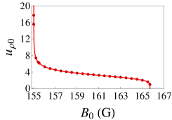
Figure 1: Equilibrium results for condensate widths $u_{\rho 0}$ (red), $u_{z0}$ (blue), and aspect ratio $u_{\rho 0}/u_{z0}$ (green) as a function of a magnetic field $B_{0}$ for different trap anisotropy (a), (c) $\lambda=0.5$ and (b) $\lambda=2$ for the experimental parameters Eq. (65). Solid, dotted, dashed, and square dotted curves correspond to the heuristic approximation of Ref. Bagnato12 and the exact results Eqs. (25)–(26) and the TF approximation Eqs. (34), (35), the TF approximation in the limit $\mathcal{H}\rightarrow\infty$ or $\varepsilon_{1}\rightarrow\infty$ results Eqs. (52), (53), respectively.

We plot in Fig. 1 the equilibrium widths of the condensate $u_{\rho 0}$, $u_{z0}$, and aspect ratio of $u_{\rho 0}/u_{z0}$ as a function of a magnetic field $B_{0}$ for the experimental parameters Eq. (65) with different trap anisotropy (a), (c) $\lambda=0.5$ and (b) $\lambda=2$. The widths of the condensate Eqs. (25) and (26) are coupled, so we solve both equations iteratively. We read off that the aspect ratio $u_{\rho 0}/u_{z0}$ turns out to coincide perfectly with the trap aspect ratio $\lambda$, therefore, it is justified to use the TF approximation Eq. (33) to find an analytical understanding for the condensate widths. From Fig. 1 we also read off that the heuristic approximation of Ref. Bagnato12 is not valid on top of the Feshbach resonance and seems to be valid only far away from the Feshbach resonance. Furthermore, Fig. 1 confirms that the TF approximation in Eqs. (36), (37) agrees quite well with the equilibrium widths determined from Eq. (25), (26) as well as the equilibrium widths calculated from the limit $\mathcal{H}$ or $\varepsilon_{1}\rightarrow\infty$. In addition Fig. 1(c) shows the radial condensate width $u_{\rho 0}$ from Eq. (25) vanishes at the critical magnetic field $B_{\rm crit}=B_{\rm res}+\Delta=165.7$ G. As already anticipated due to a heuristic argument of Ref. Bagnato12 , the system on the right-hand side of the Feshbach resonance is not stable beyond this critical magnetic field $B_{\rm crit}$.

Figures 2 and 3 show the respective frequencies of collective modes, for the experimental parameters Eq. (65) with different trap anisotropy $\lambda$. From these figures we see how the frequencies of collective modes change when one approaches the Feshbach resonance. As already expected in Eq. (9), the dipole mode frequency on the right-hand side of the Feshbach resonance turns out to be smaller than the dipole mode frequency far away from the Feshbach resonance. In particular we observe that the approximative solution of Ref. Bagnato12 is not valid on top of the Feshbach resonance. Our results and the approximative solution of Ref. Bagnato12 for the dipole mode frequency in Fig. 2 disagree only $0.05$ G above the Feshbach resonance for the experimental parameters Eq. (65). However, this is still an experimentally accessible range as the magnetic field can be controlled up to an accuracy of $1$ mG Pasquiou . Furthermore, Fig. 2(b) shows how the dipole mode frequency changes with the bias magnetic field $B_{0}$ for a hypothetical Feshbach resonance width $\Delta=100.7$ G. Thus, the difference between our predication and the approximative solution of Ref. Bagnato12 is more pronounced for a broader Feshbach resonance and for a pancake-like condensate.

Figure 2: (a) Dipole mode frequency as a function of a magnetic field $B_{0}$ for different trap anisotropy $\lambda=0.5$ (blue) and $\lambda=2$ (red) for the experimental parameters Eq. (65). Solid, dotted, dashed, and dotted square curves correspond to the approximation solution of Ref. Bagnato12 , the exact result Eq. (IV.1) and the TF approximation Eq. (43) and the TF approximation in the limit $\mathcal{H}\rightarrow\infty$ Eq. (57), respectively, while (b) focuses on the region of interest for the dipole mode frequency in addition for the hypothetical value of the Feshbach resonance $\Delta=100.7$ G, with $\lambda=0.5$ (black) and $\lambda=2$ (green).

V.2 On Top of Feshbach Resonance

We remark that approaching the Feshbach resonance and performing the TF limit represent commuting procedures within our theory. In contrast to our findings the heuristic approximation of Ref. Bagnato12 fails to predict a finite value for the dipole mode frequency on top of the Feshbach resonance aljibbouri .

Figure 4 shows the equilibrium widths of the condensate $u_{\rho 0}$, $u_{z0}$ and the aspect ratio $u_{\rho 0}/u_{z0}$ following from the exact results of Ref. aljibbouri as solid lines versus trap aspect ratio $\lambda$ and the experimental parameters Eq. (65). From Fig. 4(b) we read off that the aspect ratio $u_{\rho 0}/u_{z0}$ turns out to coincide perfectly with the trap aspect ratio $\lambda$.

In Fig. 5(a) we plot the dipole mode frequency as a function trap anisotropy $\lambda$. The solid black curve corresponds to the dipole mode frequency far away from the Feshbach resonance $\omega_{D}=\lambda$. Furthermore, the solid green curve corresponds to the exact result of dipole mode frequency on top of the Feshbah resonance aljibbouri and the dashed curve corresponds to the dipole mode in the TF approximation Eq. (49) for the experimental parameters Eq. (65). This result could be seen as being inconsistent with the Kohn theorem kohn , which says that the dipole frequency is equal to the trap frequency and does not depend on the two-body interaction strength. However, the result of the Kohn theorem is a consequence of the translational invariance of the two-body interaction, which is no longer true in our case due to Eq. (5). As a consequence the dipole mode frequency in the exact result of Ref. aljibbouri and its TF approximation Eq. (49) depend on the two-body interaction strength $\mathcal{P}_{\rm{BG}}$ and the anisotropy of the confining potential $\lambda$ both explicitly and implicitly via the equilibrium values of the condensate widths from Ref. aljibbouri .

Figure 3: Frequencies of collective modes results the quadrupole (red) and breathing (blue) as a function of a magnetic field $B_{0}$ for different trap anisotropy (a) $\lambda=0.5$ and (b) $\lambda=2$ for the experimental parameters Eq. (65). Solid, dashed, and square dotted curves correspond to the approximation solution of Ref. Bagnato12 and the TF approximation Eq. (28) with the abbreviations $m_{1}$, $m_{2}$, and $m_{3}$ from Eqs. (40)–(42) and the TF approximation in the limit $\mathcal{H}\rightarrow\infty$ or $\varepsilon_{1}\rightarrow\infty$ Eq. (28) with the abbreviations $m_{1}$, $m_{2}$, and $m_{3}$ being defined in Eqs. (54)–(56), respectively.

In Fig. 5(b) we also show the breathing (blue curves) and quadrupole (red curves) mode frequencies as a function of trap anisotropy $\lambda$. The solid curves correspond to the frequencies of collective modes far away from the Feshbach resonance, i.e. for $\varepsilon=0$, while the dashed curves correspond to the frequencies of collective mode on top of the Feshbach resonance and in the TF approximation Eqs. (28), with abbreviations $m_{1}$, $m_{2}$, and $m_{3}$ are defined in Eqs. (46)–(48) for the experimental parameters Eq. (65). We observe that approaching the Feshbach resonance leads to a significant change of the breathing mode frequency, whereas the quadrupole mode frequency remains basically unaffected.

V.3 Far Away From Feshbach Resonance

As we have $\varepsilon_{0}\rightarrow 1/\mathcal{H}$ and $\varepsilon_{1}\rightarrow\mathcal{H}$ according to (19), the results Eqs. (52)–(57) represent the $1/\mathcal{H}$ and $1/\mathcal{H}^{2}$ corrections for the respective quantities. At first we observe by comparing Eqs. (52) and (53) that the heuristic approximation of Ref. Bagnato12 reproduces correctly the $1/\mathcal{H}$ correction for the condensate widths but fails to determine the subsequent $1/\mathcal{H}^{2}$ correction. This is not surprising as the heuristic approximation (62) of Ref. Bagnato12 for the integral (13) is only exact up to order $1/\mathcal{H}$. But we read off from our results in Eq. (57) for the dipole mode frequency, plotted in Fig. 2, that the leading order correction to the Kohn theorem near Feshbach resonance is in fact of the order $1/\mathcal{H}^{2}$. Therefore, the corresponding predication of the heuristic approximation of Ref. Bagnato12 is even incorrect far away from the Feshbach resonance.

Figure 4: Equilibrium results for (a) condensate widths $u_{\rho 0}$ (red), $u_{z0}$ (blue) and (b) aspect ratio $u_{\rho 0}/u_{z0}$ (green) as a function of trap aspect ratio $\lambda$ for the experimental parameters Eq. (65). Solid and dashed curves correspond to the exact results of Ref. aljibbouri and the TF approximation Eqs. (44), (45), respectively.

In addition the similar situation for the breathing and quadrupole frequencies shows that the leading order of our results (28), with the abbreviations $m_{1}$, $m_{2}$, and $m_{3}$ from Eqs. (54)–(56), presented in Fig. 3, is $1/\mathcal{H}^{2}$ and that the frequencies depend strongly on the magnetic field $B_{0}$ and are divergent on top of the Feshbach resonance, while the frequencies of the heuristic approximation of Ref. Bagnato12 fail to determine the correct $1/\mathcal{H}^{2}$ correction and depend only on the trap anisotropy $\lambda$, i.e., they do not depend on the bias magnetic field $B_{0}$.

VI Conclusions

We have studied in detail how the dipole mode frequency and the collective excitation modes of a harmonically trapped Bose-Einstein condensate plus a bias potential change on the right-hand side and on top of the Feshbach resonance. To this end, we have derived equations of motion (16)–(18) for the variational parameters which describe the radial and axial condensate widths as well as the center of mass position and have shown how to extract the frequencies of the low-lying collective modes. At first we have analyzed our own treatment which is based on rewriting the integral in Eq. (20) with the help of the Schwinger trick schwinger . Then we have studied the consequences of this integral representation for the collective mode frequencies both on the right-hand side and on top of the Feshbach resonance.

On the right-hand side of the Feshbach resonance we found that the system is not stable beyond the critical magnetic field $B_{\rm crit}$. Furthermore, we have shown how the frequencies of the collective modes change when one approaches the Feshbach resonance. As expected initially the dipole mode frequency for the exact result and TF approximation on the right-hand side of the Feshbach resonance turn out to be smaller than the dipole mode far away from the Feshbach resonance. Furthermore we discussed the TF approximation for the condensate widths and the frequencies of collective modes in two limits. At first we considered the limit on top of the Feshbach resonance, i.e. $\mathcal{H}\rightarrow 0$ or $\varepsilon_{1}\rightarrow 0$, and afterwards, we discussed the limit far away from the Feshbach resonance, i.e. $\mathcal{H}\rightarrow\infty$ or $\varepsilon_{1}\rightarrow\infty$.

Figure 5: Frequencies of collective modes results for (a) the dipole mode frequency (green) and (b) the breathing (blue) and quadrupole (red) mode frequencies as a function of trap aspect ratio $\lambda$ for the experimental parameters Eq. (65). (a) Solid black curve corresponds to the dipole mode frequency far away the Feshbach resonance which means that $\omega_{D}=\lambda$. Solid and dashed curves correspond to the exact result of Ref. aljibbouri and in the TF approximation Eq. (49), respectively. (b) Solid and dashed curves correspond to the Eqs. (63) and in the TF approximation Eqs. (28), where the abbreviations are defined in Eqs. (46)–(48), respectively.

Our results and the approximative solution of Ref. Bagnato12 disagree for only about $0.05$ G above the Feshbach resonance for the experimental parameters of Refs. RB85 ; RB85Grimm , but this is still large enough to be experimentally accessible as the magnetic field can be tuned up to $1$ mG Pasquiou . Thus, the presented results for the violation of the Kohn theorem could, in principle, be detected in future experiments. It would be interesting to study how these results change by taking into account quantum fluctuations Arstieu1 ; Arstieu2 .

References

• (1) D. M. Stamper-Kurn, H. J. Miesner, S. Inouye, M. R. Anderws, and W. Ketterle, Phys. Rev. Lett. 81, 500 (1998).
• (2) D. S. Jin, J. R. Ensher, M. R. Matthews, C. E. Wieman, and E. A. Cornell, Phys. Rev. Lett. 77, 420 (1996).
• (3) M.-O. Mewes, M. R. Andrews, N. J. van Druten, D. M. Kurn, D. S. Durfee, C. G. Townsend, and W. Ketterle, Phys. Rev. Lett. 77, 988 (1996).
• (4) Y. Castin and R. Dum, Phys. Rev. Lett. 77, 5315 (1996).
• (5) F. Dalfovo, C. Minniti, and L. P. Pitaevskii, Phys. Rev. A. 56, 4855 (1997).
• (6) J. J. García-Ripoll, V. M. Pérez-García, and P. Torres, Phys. Rev. Lett. 83, 1715 (1999).
• (7) J. J. G. Ripoll and V. M. Pérez-García, Phys. Rev. A 59, 2220 (1999).
• (8) A. I. Nicolin, Phys. Rev. E 84, 056202 (2011).
• (9) G. Hechenblaikner, O. M. Maragò, E. Hodby, J. Arlt, S. Hopkins, and C. J. Foot, Phys. Rev. Lett. 85, 692 (2000).
• (10) E. Hodby, O.M. Maragò, G. Hechenblaikner, and C.J. Foot, Phys. Rev. Lett. 86, 2196 (2001).
• (11) Y. Zhou, W. Wen, and G. Huang, Phys Rev. B 77, 104527 (2008).
• (12) I. Vidanović, H. Al-Jibbouri, A. Balaž, and A. Pelster, Phys. Scr. T 149, 014003 (2012).
• (13) H. Al-Jibbouri, I. Vidanović, A. Balaž, and A. Pelster, J. Phys. B 46, 065303 (2013).
• (14) E. R. F. Ramos, E. A. L. Henn, J. A. Seman, M. A. Caracanhas, K. M. F. Magalhães, K. Helmerson, V. I. Yukalov, and V. S. Bagnato, Phys. Rev. A 78, 063412 (2008).
• (15) S. E. Pollack, D. Dries, M. Junker, Y. P. Chen, T. A. Corcovilos, and R. G. Hulet, Phys. Rev. Lett. 102, 090402 (2009).
• (16) S. E. Pollack, D. Dries, R. G. Hulet, K. M. F. Magalhães, E. A. L. Henn, E. R. F. Ramos, M. A. Caracanhas, and V. S. Bagnato, Phys. Rev. A 81, 053627 (2010).
• (17) I. Vidanović, A. Balaž, H. Al-Jibbouri, and A. Pelster, Phys. Rev. A 84, 013618 (2011).
• (18) S. Sabari, R. V. J. Raja, K. Porsezian and P. Muruganandam, J. Phys. B: At. Mol. Opt. Phys. 43, 125302 (2010).
• (19) A. I. Nicolin, Rom. Rep. Phys., 63, 1329 (2011).
• (20) W. Cairncross and A. Pelster, arXiv:1209.3148.
• (21) W. Kohn, Phys. Rev. 123, 1242 (1961).
• (22) A. L. Fetter and D. Rokhsar, Phys. Rev. A 57, 1191 (1998).
• (23) E. Zaremba, T. Nikuni, and A. Griffin, J. Low Temp. Phys. 116, 277 (1999).
• (24) M. J. Bijlsma and H. T. C. Stoof, Phys. Rev. A 60, 3973 (1999).
• (25) A. Minguzzi and M. P. Tosi, J. Phys.: Condens. Matter 9, 10211 (1997).
• (26) J. Reidl, G. Bene, R. Graham, and P. Szépfalusy, Phys. Rev. A 63, 043605 (2001).
• (27) A. Minguzzi, Phys. Rev. A 64, 033604 (2001).
• (28) T. Maruyama and G. F. Bertsch, Phys. Rev. A 77, 063611 (2008).
• (29) A. Banerjee, J. Phys. B: At. Mol. Opt. Phys. 42, 235301 (2009).
• (30) J.-Y. Zhang, S.-C. Ji, Z. Chen, L. Zhang, Z.-D. Du, B. Yan, G.-S. Pan, B. Zhao, Y.-J. Deng, H. Zhai, S. Chen, and J.-W. Pan, Phys. Rev. Lett. 109, 115301 (2012).
• (31) Y. Li, G. I. Martone, and S. Stringari, Euro. Phys. Lett. 99, 56008 (2012).
• (32) F. Ferlaino, R. J. Brecha, P. Hannaford, F. Riboli, G. Roati, G. Modugno, and M. Inguscio, J. Opt. B: Quantum Semiclass. Opt. 5, S3 (2003).
• (33) S. Chiacchiera, T. Macrìand A. Trombettoni, Phys. Rev. A 81, 033624 (2010).
• (34) Y. Lu, W. Xiao-Rui, L. Ke, T. Xin-Zhou, X. Hong-Wei, and L. Bao-Long, Chin. Phys. Lett. 26, 076701 (2009).
• (35) S. Stringari, Phys. Rev. Lett. 77, 2360 (1996).
• (36) C. J. Pethick and H. Smith, Bose-Einstein Condensation in Dilute Gases, 2nd edition (Cambridge University Press, Cambridge, 2008).
• (37) H. Ott, J. Fortágh, S. Kraft, A. Günther, D. Komma, and C. Zimmermann, Phys. Rev. Lett. 91, 040402 (2003).
• (38) E. R. F. Ramos, F. E. A. dos Santos, M. A. Caracanhas, and V. S. Bagnato, Phys. Rev. A 85, 033608 (2012).
• (39) T. Esslinger, I. Bloch, and T. W. Hansch, Phys. Rev. A 58, R2664 (1998).
• (40) P. A. Altin, N. P. Robins, D. Döring, J. E. Debs, R. Poldy, C. Figl, and J. D. Close, Rev. Sci. Instrum. 81, 063103 (2010).
• (41) C. Chin, R. Grimm, P. Julienne, and E. Tiesinga, Rev. Mod. Phys. 82, 1225 (2010).
• (42) E. P. Gross, Nuovo Cimento, 20, 454 (1961).
• (43) L. P. Pitaevskii, Sov Phys. JETP 13, 451 (1961).
• (44) V. M. Pérez-García, H. Michinel, J . I. Cirac, M. Lewenstein, and P. Zoller, Phys. Rev. Lett. 77, 5320 (1996).
• (45) V. M. Pérez-García, H. Michinel, J. I. Cirac, M. Lewenstein, P. Zoller, Phys. Rev. A 56, 1424 (1997).
• (46) H. Kleinert and V. Schulte-Frohlinde, Critical Properties of $\Phi^{4}$-Theories (World Scientific, Singapore, 2001).
• (47) A. J. Moerdijk, B. J. Verhaar, and A. Axelsson, Phys. Rev. A 51, 4852 (1995).
• (48) S. Yi and L. You, Phys. Rev. A 67, 045601 (2003).
• (49) Mathematica symbolic calculation software package, http://www.wolfram.com/mathematica.
• (50) B. Pasquiou, E. Maréchal, G. Bismut, P. Pedri, L. Vernac, O. Gorceix, and B. Laburthe-Tolra, Phys. Rev. Lett. 106, 255303 (2011).
• (51) H. Al-Jibbouri, Collective Excitations in Bose-Einstein Condensates, PhD thesis, Free University of Berlin, In preparation.
• (52) A. R. P. Lima and A. Pelster, Phys. Rev. A 84, 041604 (2011).
• (53) A. R. P. Lima and A. Pelster, Phys. Rev. A 86, 063609 (2012).