Sign-preserving of principal eigenfunctions in P1 finite element approximation of eigenvalue problems of second-order elliptic operators

Abstract

This paper is concerned with the P1 finite element approximation of the eigenvalue problem of second-order elliptic operators subject to the Dirichlet boundary condition. The focus is on the preservation of basic properties of the principal eigenvalue and eigenfunctions of continuous problems. It is shown that when the stiffness matrix is an irreducible $M$-matrix, the algebraic eigenvalue problem maintains those properties such as the smallest eigenvalue being real and simple and the corresponding eigenfunctions being either positive or negative inside the physical domain. Mesh conditions leading to such a stiffness matrix are also studied. A sufficient condition is that the mesh is simplicial, acute when measured in the metric specified by the inverse of the diffusion matrix, and interiorly connected. The acute requirement can be replaced by the Delaunay condition in two dimensions. Numerical results are presented to verify the theoretical findings.

AMS 2010 Mathematics Subject Classification. 65N25, 65N30, 65N30

Key Words. finite element method, eigenvalue problem, sign-preserving, positivity-preserving, Perron’s theorem.

Abbreviated title. Sign-preserving of principal eigenfunctions in FEM

1 Introduction

We are concerned with the P1 finite element approximation of the eigenvalue problem of a general second-order elliptic operator

$$\begin{cases}Lu\equiv-\nabla\cdot(\mathbb{D}\,\nabla u)+\mbox{\boldmath$b$}\cdot\nabla u+c\,u=\lambda u,&\quad\mbox{ in }\Omega\\ u=0,&\quad\mbox{ on }\partial\Omega\end{cases}$$ (1)

where $\Omega\subset\mathbb{R}^{d}$ ($d\geq 1$) is a polyhedron and $\mathbb{D}=\mathbb{D}(\mbox{\boldmath$x$}):\Omega\to\mathbb{R}^{d\times d}$, $\mbox{\boldmath$b$}=\mbox{\boldmath$b$}(\mbox{\boldmath$x$}):\Omega\to\mathbb{R}^{d}$, and $c=c(\mbox{\boldmath$x$}):\Omega\to\mathbb{R}$ are given, sufficiently smooth functions. We assume that $\mathbb{D}$ is symmetric and strictly positive definite on $\Omega$ and the functions $b$ and $c$ satisfy

$$c(\mbox{\boldmath$x$})-\frac{1}{2}\nabla\cdot\mbox{\boldmath$b$}(\mbox{\boldmath$x$})\geq 0,\qquad\forall\mbox{\boldmath$x$}\in\Omega.$$ (2)

Note that the condition (2) is not essential. We can always make them satisfied by adding a large positive number to the function $c(\mbox{\boldmath$x$})$. The original and shifted problems will have the same eigenfunctions and the eigenvalues of the former can be obtained by shifting the eigenvalues of the latter.

The eigenvalue problem (1) is not self-adjoint in general. Nevertheless, it is known (e.g., see Lemma 3.1 below or Evans [27, Theorem 2 on Page 336 and Theorem 3 on page 340]) that the principal eigenvalue (that is, the smallest eigenvalue in modulus) is real and simple and the principal eigenfunctions (that is, the eigenfunctions corresponding to the principal eigenvalue) are either positive or negative in $\Omega$. Since the principal eigenvalues typically represent the ground state of a physical system or correspond to the most unstable mode in stability or sensitivity analysis, it is of practical and theoretical importance to study when a numerical approximation preserves these properties of the principal eigenvalue and eigenfunctions and especially the sign of the principal eigenfunctions.

The objective of this paper is to investigate when a P1 finite element approximation of (1) on a simplicial mesh preserves the basic properties of the principal eigenvalue and eigenfunctions of the continuous problem. We shall show that most of the basic properties of the principal eigenvalue and eigenfunctions are preserved in the P1 finite element approximation provided that the resulting stiffness matrix is an irreducible $M$-matrix (cf. Theorem 3.1). Particularly, the principal eigenvalue of the discrete system is real and algebraically and geometrically simple and the corresponding eigenfunctions are either positive or negative (sign-preserving) in the physical domain. Several sufficient mesh conditions are proposed (Theorem 4.1) for the stiffness matrix to be an irreducible $M$-matrix.

We point out that there is a vast literature on the finite element approximation of differential eigenvalue problems and most of it is on convergence analysis; e.g., see Babuška and Osborn [2], Boffi [8], and Boffi et al. [9], and references therein. Early work includes Birkhoff et al. [7], Fix [28], and Babuška and Osborn [3]. We also point out some interesting recent work [20, 21, 35, 51, 52, 54, 62, 65, 66].

An outline of the paper is as follows. The P1 finite element approximation of (1) is presented in §2 and the preservation of the basic properties of the principal eigenvalue and eigenfunctions in the P1 finite element approximation is studied in §3. §4 is devoted to the study of mesh conditions under which the stiffness matrix is ensured to be an irreducible $M$-matrix, followed by numerical examples in §5. The conclusions are drawn in §6.

2 P1 finite element formulation

The weak formulation of the eigenvalue problem (1) is to find $\lambda\in\mathbb{C}$ and nonzero (and possibly complex) function $u\in H_{0}^{1}(\Omega)$ such that

$$(\mathbb{D}\nabla u,\nabla v)+(\mbox{\boldmath$b$}\cdot\nabla u,v)+(c\,u,v)=\lambda(u,v),\quad\forall v\in H_{0}^{1}(\Omega)$$ (3)

where $(\cdot,\cdot)$ denotes the $L^{2}$ inner product. For the P1 finite element approximation, we assume that an affine family of simplicial mesh $\{\mathcal{T}_{h}\}$ is given for $\Omega$. Denote by $V^{h}\subset H_{0}^{1}(\Omega)$ the standard P1 finite element space associated with a mesh $\mathcal{T}_{h}$. A P1 finite element approximation to the eigenvalue problem (3) is to find $\lambda^{h}\in\mathbb{C}$ and nonzero (and possibly complex) function $u^{h}\in V^{h}$ such that

$$(\mathbb{D}\nabla u^{h},\nabla v^{h})+(\mbox{\boldmath$b$}\cdot\nabla u^{h},v^{h})+(c\,u^{h},v^{h})=\lambda^{h}(u^{h},v^{h}),\quad\forall\;v^{h}\in V^{h}.$$ (4)

Scheme (4) can be expressed in a matrix form. Denote the numbers of the elements and the interior vertices of $\mathcal{T}_{h}$ by $N$ and $N_{v}$, respectively. Assume that the vertices are ordered in such a way that the first $N_{v}$ vertices are the interior ones. Then, $V^{h}$ and $u^{h}$ can be expressed as

$$V^{h}=\text{span}\{\phi_{1},\cdots,\phi_{N_{v}}\},\quad u^{h}=\sum_{k=1}^{N_{v}}u_{k}\phi_{k},$$

where $\phi_{k}$ denotes the P1 basis function associated with the $k^{\text{th}}$ vertex. Substituting the above expression into (4) and taking $v^{h}=\phi_{j}$ ($j=1,...,N_{v}$), we obtain the algebraic eigenvalue problem

$$A\,\mbox{\boldmath$u$}=\lambda^{h}B\mbox{\boldmath$u$},$$ (5)

where $\mbox{\boldmath$u$}=(u_{1},...,u_{N_{v}})^{T}$, the stiffness matrix $A$ and the mass matrix $B$ are given by

$$A_{jk}=\sum_{K\in\mathcal{T}_{h}}\int_{K}d\mbox{\boldmath$x$}\left(\frac{}{}(\nabla\phi_{j})^{T}\,\mathbb{D}_{K}\,\nabla\phi_{k}+\phi_{j}\;(\mbox{\boldmath$b$}\cdot\nabla\phi_{k})+c\;\phi_{j}\,\phi_{k}\right),\quad j,k=1,...,N_{v}$$ (6)

$$B_{jk}=\sum_{K\in\mathcal{T}_{h}}\int_{K}\phi_{j}\phi_{k}d\mbox{\boldmath$x$},\quad j,k=1,...,N_{v}$$ (7)

and $\mathbb{D}_{K}$ is the average of $\mathbb{D}$ over $K$, i.e.,

$$\mathbb{D}_{K}=\frac{1}{|K|}\int_{K}\mathbb{D}(\mbox{\boldmath$x$})\,d\mbox{\boldmath$x$}.$$ (8)

The convergence of finite element approximation of (3) has been extensively studied (e.g., see [8]). We can expect that the principal eigenvalue of (4) converges to that of the continuous problem (3) at $\mathcal{O}(N^{-\frac{2}{d}})$ (second order) as $N\to\infty$. On the other hand, the preservation of the basic properties of the principal eigenvalue and eigenfunctions by the discrete system has not been studied so far (to our best knowledge). Our goal is to establish conditions (on the stiffness matrix and the mesh) under which the discrete eigenvalue problem (5) preserves those properties.

3 Preservation of basic properties of the principal eigenvalue and eigenfunctions

In this section we describe basic properties of the principal eigenvalue and eigenfunctions of the continuous problem (3) (Lemma 3.1) and show (Theorem 3.1) that those properties are preserved by the discrete eigenvalue problem (4) provided that the stiffness matrix $A$ is an irreducible $M$-matrix. The mesh conditions to ensure an irreducible $M$-matrix stiffness matrix for the P1 finite element approximation will be studied in the next section.

      Lemma 3.1.

The principal eigenvalue $\lambda_{1}$ and the corresponding eigenfunctions of the eigenvalue problem (3) have the following properties.

• $\lambda_{1}$ is real;

• There is an eigenfunction $u_{1}\in H_{0}^{1}(\Omega)$ associated with $\lambda_{1}$ with $u_{1}(\mbox{\boldmath$x$})>0$ for all $\mbox{\boldmath$x$}\in\Omega$;

• $\lambda_{1}$ is simple, that is, if $u$ is an eigenfunction associated with $\lambda_{1}$, then $u$ is a multiple of $u_{1}$;

• $\lambda_{1}=F(u_{1})>0$, where $F(\cdot)$ is defined as

  $$F(v)=\frac{(\mathbb{D}\nabla v,\nabla v)+((c-\frac{1}{2}\nabla\cdot\mbox{\boldmath$b$})v,v)}{(v,v)};$$ (9)

• $\text{Re}(\lambda)\geq\lambda_{1}$ for every eigenvalue $\lambda$;

• For the symmetric situation (with $\mbox{\boldmath$b$}=0$), there holds the variational principle

  $$\lambda_{1}=\min\limits_{\begin{subarray}{c}v\in H_{0}^{1}(\Omega)\\ v\not\equiv 0,\;\text{real}\end{subarray}}F(v).$$ (10)

Proof. (a), (b), (c), (e), and (f) are the standard results for second-order elliptic operators; e.g, see [27, Theorem 2 on Page 336 and Theorem 3 on page 340]. (d) follows from equation (3) (with $u=v=u_{1}$), integration by parts, the assumption (2), Poincaré’s inequality, and the fact that $\lambda_{1}$ and $u_{1}$ are real.

      Theorem 3.1.

For the finite element eigenvalue problem (4), if the stiffness matrix $A$ is an irreducible $M$-matrix, then the principal eigenvalue $\lambda_{1}^{h}$ and the corresponding eigenfunctions have the following properties.

• $\lambda_{1}^{h}$ is real;

• There is an eigenfunction $u_{1}^{h}\in V^{h}$ associated with $\lambda_{1}^{h}$ with $u_{1}^{h}(\mbox{\boldmath$x$})>0$ for all $\mbox{\boldmath$x$}\in\Omega$;

• $\lambda_{1}^{h}$ is algebraically (and geometrically) simple, that is, if $u^{h}$ is an eigenfunction associated with $\lambda_{1}^{h}$, then $u^{h}$ is a multiple of $u_{1}^{h}$;

• $\lambda_{1}^{h}=F(u_{1}^{h})>0$, where $F(\cdot)$ is defined in (9);

• $\text{Re}(\lambda^{h})>0$ and $|\lambda^{h}|\geq\lambda_{1}$ for every eigenvalue $\lambda^{h}$;

• For the symmetric situation (with $\mbox{\boldmath$b$}=0$), there holds the variational principle

  $$\lambda_{1}^{h}=\min\limits_{\begin{subarray}{c}v^{h}\in V^{h}\\ v^{h}\not\equiv 0,\;\text{real}\end{subarray}}F(v^{h}).$$ (11)

Proof. The finite element eigenvalue problem (4) or (5) is mathematically equivalent to

$$A^{-1}B\mbox{\boldmath$u$}=\frac{1}{\lambda^{h}}\mbox{\boldmath$u$}.$$ (12)

Since $A$ is an irreducible $M$-matrix, $A^{-1}$ is positive, i.e., $A^{-1}>0$ (in the elementwise sense). From (7), it is obvious that each column of $B$ has at least one non-zero entry. Thus, we have $A^{-1}B>0$. We also notice that $u^{h}(\mbox{\boldmath$x$})=\sum_{j=1}^{N_{v}}u_{j}\phi_{j}(\mbox{\boldmath$x$})>0$ for all $\mbox{\boldmath$x$}\in\Omega$ if and only if $\mbox{\boldmath$u$}=(u_{1},...,u_{N_{v}})^{T}>0$. Then, (a), (b), and (c) follow from Perron’s Theorem (for positive matrices; e.g., see [34, 8.2.11]). (d) follows from the equation (4) (with $u^{h}=v^{h}=u_{1}^{h}$), integration by parts, the assumption (2), Poincaré’s inequality, and the fact that $\lambda_{1}^{h}$ and $u_{1}^{h}$ are real. For (e), the property $\text{Re}(\lambda^{h})>0$ is a consequence of the fact that $A$ is an $M$-matrix and $B$ is a symmetric and positive definite matrix. The other property follows from Perron’s Theorem.

Next, we show that (f) holds. For this case, $A$ is symmetric. From Perron’s Theorem, the eigenvalues of (5) can be ordered as

$$0<\lambda_{1}^{h}<\lambda_{2}^{h}\leq\cdots\leq\lambda_{N_{v}}^{h}.$$

Denote the corresponding normalized eigenvectors by $u_{j}^{h}$ (or $\mbox{\boldmath$u$}_{j}$ in vector form) ($j=1,...,N_{v}$). Notice that they satisfy $\mbox{\boldmath$u$}_{j}^{T}B\mbox{\boldmath$u$}_{k}=\delta_{jk}$. Then, any function $v^{h}\in V^{h}$ can be expressed into

$$v^{h}=\sum_{j=1}^{N_{v}}d_{j}u_{j}^{h}\quad\text{ or }\quad\mbox{\boldmath$v$}=\sum_{j=1}^{N_{v}}d_{j}\mbox{\boldmath$u$}_{j}.$$

From the orthogonality of the eigenfunctions, we have

$$F(v^{h})=\frac{\mbox{\boldmath$v$}^{T}A\mbox{\boldmath$v$}}{\mbox{\boldmath$v$}^{T}B\mbox{\boldmath$v$}}=\frac{\sum_{j}d_{j}^{2}\lambda_{j}^{h}}{\sum_{j}d_{j}^{2}}\geq\lambda_{1}^{h}.$$

Combining this with (d) gives (11).

      Remark 3.1.

We note that the properties in Theorem 3.1(e) are different from the stronger property $\text{Re}(\lambda^{h})\geq\lambda_{1}^{h}$ (cf. Lemma 3.1(e)). There are two cases we can show that the discrete system has the latter property when $A$ is an irreducible $M$-matrix. The first case is the symmetric case. In this case, $\text{Re}(\lambda^{h})=\lambda^{h}$, and $\text{Re}(\lambda^{h})>0$ and $|\lambda^{h}|\geq\lambda_{1}$ imply $\text{Re}(\lambda^{h})\geq\lambda_{1}^{h}$. The other case is to use the lumped mass matrix (denoted by $\tilde{B}$) instead of the full mass matrix $B$. Since $\tilde{B}$ is diagonal, $\tilde{B}^{-1}A$ is also an irreducible $M$-matrix, which implies $\text{Re}(\lambda^{h})\geq\lambda_{1}^{h}$ (e.g., see Elhashash and Szyld [25, Theorem 3.1]).

For the general nonsymmetric situation, we are unable to show that the discrete system has the property $\text{Re}(\lambda^{h})\geq\lambda_{1}^{h}$ for every eigenvalue $\lambda^{h}$ although our limited numerical experiment shows that the system does satisfy the property (cf. Fig. 5).

Theorem 3.1 states that if $A$ is an irreducible $M$-matrix, then the P1 finite element approximation (4) essentially retains most of the properties listed in Lemma 3.1 for the principal eigenvalue and eigenfunctions. In the next section we study the mesh conditions to ensure that the P1 finite element stiffness matrix be an irreducible $M$-matrix.

4 Mesh conditions for irreducible $M$-matrix stiffness matrix

We first study mesh conditions to ensure $A$ to be an $M$-matrix. This issue is closely related to the preservation of the maximum principle for boundary value problems. The latter has been studied extensively in the past; for example, see [13, 15, 17, 19, 40, 41, 43, 45, 59, 60, 61, 63] for isotropic diffusion problems ($\mathbb{D}=\alpha(\mbox{\boldmath$x$})I$ with $\alpha(\mbox{\boldmath$x$})$ being a scalar function) and [24, 30, 31, 38, 42, 44, 46, 47, 48, 49, 50, 53, 57, 58, 67, 68] for anisotropic diffusion problems.

In the following we quote a result from Lu et al. [50]. We first introduce some notation. For any simplicial element $K$, we denote the inner normal to face $S_{j}^{K}$ (the face not containing the $j^{\text{th}}$ vertex of $K$) by $\mbox{\boldmath$q$}_{j}^{K}$. The dihedral angle in the metric $\mathbb{D}^{-1}$ between faces $S_{j}^{K}$ and $S_{k}^{K}$ ($j\neq k$) can be computed as

$$\alpha_{jk,\mathbb{D}^{-1}}^{K}=-\frac{(\mbox{\boldmath$q$}_{j}^{K})^{T}\mathbb{D}_{K}\mbox{\boldmath$q$}_{k}^{K}}{\sqrt{(\mbox{\boldmath$q$}_{j}^{K})^{T}\mathbb{D}_{K}\mbox{\boldmath$q$}_{j}^{K}\cdot(\mbox{\boldmath$q$}_{k}^{K})^{T}\mathbb{D}_{K}\mbox{\boldmath$q$}_{k}^{K}}}.$$ (13)

The maximum dihedral angle in the metric $\mathbb{D}^{-1}$ for $K$ is defined as

$$\alpha_{\max,\mathbb{D}^{-1}}^{K}=\max\limits_{j,k=1,...,d+1,j\neq k}\alpha_{jk,\mathbb{D}^{-1}}^{K}.$$ (14)

The diameter (i.e., the largest edge length in the Euclidean metric) of $K$ is denoted by $h_{K}$.

      Lemma 4.1.

If the mesh satisfies

$$0<\alpha_{\max,\mathbb{D}^{-1}}^{K}\leq\arccos\left(\frac{h_{K}}{\lambda_{min}(\mathbb{D}_{K})}\cdot\frac{\|\mbox{\boldmath$b$}\|_{L^{\infty}(K)}}{(d+1)}+\frac{h_{K}^{2}}{\lambda_{min}(\mathbb{D}_{K})}\cdot\frac{\|c\|_{L^{\infty}(K)}}{(d+1)(d+2)}\right),\quad\forall K\in\mathcal{T}_{h}$$ (15)

then, the stiffness matrix $A$ is an $M$-matrix.

In 2D, the above condition can be replaced by a Delaunay-type condition

$$0<\frac{1}{2}\left[\frac{}{}\alpha_{jk,\mathbb{D}^{-1}}^{K}+\alpha_{jk,\mathbb{D}^{-1}}^{K^{\prime}}\right.$$

$$\quad+\text{ arccot}\left(\sqrt{\frac{\mbox{ det}(\mathbb{D}_{K^{\prime}})}{\mbox{ det}(\mathbb{D}_{K})}}\cot(\alpha_{jk,\mathbb{D}^{-1}}^{K^{\prime}})-\frac{2\;\Theta(K,K^{\prime})}{\sqrt{\mbox{ det}(\mathbb{D}_{K})}}\right)$$

$$\quad\left.+\text{ arccot}\left(\sqrt{\frac{\mbox{ det}(\mathbb{D}_{K})}{\mbox{ det}(\mathbb{D}_{K^{\prime}})}}\cot(\alpha_{jk,\mathbb{D}^{-1}}^{K})-\frac{2\;\Theta(K,K^{\prime})}{\sqrt{\mbox{ det}(\mathbb{D}_{K^{\prime}})}}\right)\frac{}{}\right]\leq\pi$$ (16)

for every internal edge $e_{jk}$ connecting the $j^{\text{th}}$ and $k^{\text{th}}$ vertices. Here, $K$ and $K^{\prime}$ are the elements sharing the common edge $e_{jk}$, $\alpha_{jk,\mathbb{D}^{-1}}^{K}$ and $\alpha_{jk,\mathbb{D}^{-1}}^{K^{\prime}}$ are the angles in $K$ and $K^{\prime}$ that face the edge, and

$$\Theta(K,K^{\prime})=\frac{h_{K}\;\|\mbox{\boldmath$b$}\|_{L^{\infty}(K)}}{(d+1)}+\frac{h_{K}^{2}\;\|c\|_{L^{\infty}(K)}}{(d+1)(d+2)}+\frac{h_{K^{\prime}}\;\|\mbox{\boldmath$b$}\|_{L^{\infty}(K)}}{(d+1)}+\;\frac{h_{K^{\prime}}^{2}\;\|c\|_{L^{\infty}(K)}}{(d+1)(d+2)}.$$ (17)

Proof. This result was proven in Lu et al. [50, Theorems 1 and 2]. For completeness, we give a proof here. The proof is also useful in the study of irreducibility of the stiffness matrix, see Theorem 4.1.

We first show that $A$ is a Z-matrix; i.e.,

$$a_{jk} \leq 0,\;\;\forall\;j\neq k,\;j,k=1,...,N_{v}$$

$$a_{jj} \geq 0,\;\;j=1,...,N_{v}.$$

Recall from Ciarlet [18, Page 201] that

$$\int\limits_{K\in\omega_{j}}\phi_{j}d\mbox{\boldmath$x$}=\frac{|K|}{d+1},\quad\int\limits_{K\in\omega_{j}\cap\omega_{k}}\phi_{j}\phi_{k}d\mbox{\boldmath$x$}=\frac{|K|}{(d+1)(d+2)},\quad j\neq k$$ (18)

where $\omega_{j}$ and $\omega_{k}$ are the element patches associated with the $j^{\text{th}}$ and $k^{\text{th}}$ vertices, respectively. For $j\neq k$, from (6) we have

$$a_{jk}=\sum_{K\in\omega_{j}\cap\omega_{k}}\left(|K|\;(\nabla\phi_{j})^{T}\;\mathbb{D}_{K}\;\nabla\phi_{k}+\int_{K}\;\phi_{j}\;(\mbox{\boldmath$b$}\cdot\nabla\phi_{k})d\mbox{\boldmath$x$}+\;\int_{K}\;c\;\phi_{j}\;\phi_{k}d\mbox{\boldmath$x$}\right).$$

From [50, Lemmas 1 and 3],

$$\left.\nabla\phi_{j}\right|_{K}=-\frac{1}{h_{j}^{K}}\frac{\mbox{\boldmath$q$}_{j}^{K}}{\sqrt{(\mbox{\boldmath$q$}_{j}^{K})^{T}\mbox{\boldmath$q$}_{j}^{K}}},\quad\left.(\nabla\phi_{j})^{T}\;\mathbb{D}_{K}\;\nabla\phi_{k}\right|_{K}=-\frac{\cos(\alpha_{jk,\mathbb{D}^{-1}}^{K})}{h_{j,\mathbb{D}^{-1}}^{K}h_{k,\mathbb{D}^{-1}}^{K}},$$

where $h_{j}^{K}$ and $h_{j,\mathbb{D}^{-1}}^{K}$ are the $j^{\text{th}}$ altitude of $K$ in the Euclidean metric and the metric specified by $\mathbb{D}^{-1}$, respectively. They are related by

$$\frac{h_{j}^{K}}{\sqrt{\lambda_{\max}(\mathbb{D}_{K})}}\leq h_{j,\mathbb{D}^{-1}}^{K}\leq\frac{h_{j}^{K}}{\sqrt{\lambda_{\min}(\mathbb{D}_{K})}}.$$

Combining the above results, we have

$$a_{jk} \leq\sum_{K\in\omega_{j}\cap\omega_{k}}\left(-\frac{|K|}{h_{j,\mathbb{D}^{-1}}^{K}h_{k,\mathbb{D}^{-1}}^{K}}\cos(\alpha_{jk,\mathbb{D}^{-1}}^{K})+\frac{\|\mbox{\boldmath$b$}\|_{L^{\infty}(K)}}{h_{k}^{K}}\int_{K}\phi_{j}d\mbox{\boldmath$x$}+\|c\|_{L^{\infty}(K)}\int_{K}\;\phi_{j}\;\phi_{k}\;d\mbox{\boldmath$x$}\right)$$

$$=\sum_{K\in\omega_{j}\cap\omega_{k}}\left(-\frac{|K|}{h_{j,\mathbb{D}^{-1}}^{K}h_{k,\mathbb{D}^{-1}}^{K}}\cos(\alpha_{jk,\mathbb{D}^{-1}}^{K})+\frac{|K|\;\|\mbox{\boldmath$b$}\|_{L^{\infty}(K)}}{(d+1)h_{k}^{K}}+\frac{|K|\;\|c\|_{L^{\infty}(K)}}{(d+1)(d+2)}\right)$$

$$=\sum_{K\in\omega_{j}\cap\omega_{k}}\frac{|K|}{h_{j,\mathbb{D}^{-1}}^{K}h_{k,\mathbb{D}^{-1}}^{K}}\left(-\cos(\alpha_{jk,\mathbb{D}^{-1}}^{K})+\frac{h_{j,\mathbb{D}^{-1}}^{K}h_{k,\mathbb{D}^{-1}}^{K}\|\mbox{\boldmath$b$}\|_{L^{\infty}(K)}}{(d+1)h_{k}^{K}}+\frac{h_{j,\mathbb{D}^{-1}}^{K}h_{k,\mathbb{D}^{-1}}^{K}\|c\|_{L^{\infty}(K)}}{(d+1)(d+2)}\right)$$

$$\leq\sum_{K\in\omega_{j}\cap\omega_{k}}\frac{|K|}{h_{j,\mathbb{D}^{-1}}^{K}h_{k,\mathbb{D}^{-1}}^{K}}\left(-\cos(\alpha_{\max,\mathbb{D}^{-1}}^{K})+\frac{h_{K}\|\mbox{\boldmath$b$}\|_{L^{\infty}(K)}}{(d+1)\lambda_{\min}(\mathbb{D}_{K})}+\frac{h_{K}^{2}\|c\|_{L^{\infty}(K)}}{(d+1)(d+2)\lambda_{\min}(\mathbb{D}_{K})}\right).$$ (19)

Thus, $a_{j,k}\leq 0$ when (15) is satisfied.

In two dimensions, notice that there are only two elements in $\omega_{j}\cap\omega_{k}$ which share the common edge $e_{jk}$. Denote these elements by $K$ and $K^{\prime}$. Similarly, we can get

$$a_{jk} \leq-\frac{\mbox{det}(\mathbb{D}_{K})^{\frac{1}{2}}}{2}\cot(\alpha_{jk,\mathbb{D}^{-1}}^{K})-\frac{\mbox{det}(\mathbb{D}_{K^{\prime}})^{\frac{1}{2}}}{2}\cot(\alpha_{jk,\mathbb{D}^{-1}}^{K^{\prime}})$$

$$\quad+\frac{h_{K}\;\|\mbox{\boldmath$b$}\|_{L^{\infty}(K)}}{(d+1)}+\frac{h_{K}^{2}\;\|c\|_{L^{\infty}(K)}}{(d+1)(d+2)}+\frac{h_{K^{\prime}}\;\|\mbox{\boldmath$b$}\|_{L^{\infty}(K^{\prime})}}{(d+1)}+\frac{h_{K^{\prime}}^{2}\;\|c\|_{L^{\infty}(K^{\prime})}}{(d+1)(d+2)}.$$ (20)

It can be shown (e.g., see [38]) that $a_{jk}\leq 0$ when (16) is satisfied.

For the diagonal entries, we have

$$a_{jj} =\sum_{K\in\mathcal{T}_{h}}|K|\;(\nabla\phi_{i})^{T}\;\mathbb{D}_{K}\;\nabla\phi_{i}+\int_{\Omega}\;\phi_{i}\;(\mbox{\boldmath$b$}\cdot\nabla\phi_{i})d\mbox{\boldmath$x$}+\int_{\Omega}\;c\;\phi_{i}^{2}d\mbox{\boldmath$x$}$$

$$\geq\int_{\Omega}\phi_{i}(\mbox{\boldmath$b$}\cdot\nabla\phi_{i})d\mbox{\boldmath$x$}+\int_{\Omega}c\;\phi_{i}^{2}d\mbox{\boldmath$x$}=\int_{\Omega}(c-\frac{1}{2}\nabla\cdot\mbox{\boldmath$b$})\phi_{i}^{2}d\mbox{\boldmath$x$}\geq 0.$$

Thus, $A$ is a Z-matrix.

We now show that $A$ is an M-matrix by showing that $A$ is positive definite. For any vector $\mbox{\boldmath$v$}=(v_{1},v_{2},...,v_{N_{v}})^{T}$, we define $v^{h}=\sum_{i=1}^{N_{v}}v_{i}\phi_{i}\in V^{h}$. Notice that $\nabla v^{h}$ is constant on $K$. As in the proof for $a_{jj}\geq 0$, from (6) we have

$$\mbox{\boldmath$v$}^{T}A\mbox{\boldmath$v$} = \sum_{K\in\mathcal{T}_{h}}|K|\;(\nabla v^{h})^{T}\;\mathbb{D}_{K}\;\nabla v^{h}+\int_{\Omega}v^{h}\;(\mbox{\boldmath$b$}\cdot\nabla v^{h})d\mbox{\boldmath$x$}+\int_{\Omega}c\;(v^{h})^{2}d\mbox{\boldmath$x$}$$

$$= \int_{\Omega}\;(\nabla v^{h})^{T}\;\mathbb{D}\;\nabla v^{h}d\mbox{\boldmath$x$}+\int_{\Omega}(c-\frac{1}{2}\nabla\cdot\mbox{\boldmath$b$})(v^{h})^{2}d\mbox{\boldmath$x$}\geq 0.$$

Moreover, from the above inequality it is easy to see that $\mbox{\boldmath$v$}^{T}A\mbox{\boldmath$v$}=0$ implies

$$\int_{\Omega}\;(\nabla v^{h})^{T}\;\mathbb{D}\;\nabla v^{h}d\mbox{\boldmath$x$}=0.$$

We thus have $\nabla v^{h}=0$ or $v^{h}=$ constant, which in turn implies $v^{h}=0$ due to the fact that $v^{h}$ vanishes on $\partial\Omega$. Hence, $A$ is positive definite.

      Remark 4.1.

Loosely speaking, the mesh conditions (15) and (16) can be written as

$$0<\, \alpha_{\max,\mathbb{D}^{-1}}^{K}\leq\frac{\pi}{2}-C_{1}\|\mbox{\boldmath$b$}\|_{L^{\infty}(\Omega)}h-C_{2}\|c\|_{L^{\infty}(\Omega)}h^{2},\quad\forall K\in\mathcal{T}_{h}$$ (21)

$$0<\, \frac{1}{2}\left[\frac{}{}\alpha_{jk,\mathbb{D}^{-1}}^{K}+\alpha_{jk,\mathbb{D}^{-1}}^{K^{\prime}}+\text{ arccot}\left(\sqrt{\frac{\mbox{ det}(\mathbb{D}_{K^{\prime}})}{\mbox{ det}(\mathbb{D}_{K})}}\cot(\alpha_{jk,\mathbb{D}^{-1}}^{K^{\prime}})\right)\right.$$

$$\left.+\text{ arccot}\left(\sqrt{\frac{\mbox{ det}(\mathbb{D}_{K})}{\mbox{ det}(\mathbb{D}_{K^{\prime}})}}\cot(\alpha_{jk,\mathbb{D}^{-1}}^{K})\right)\frac{}{}\right]$$

$$\qquad\qquad\leq\pi-C_{3}\|\mbox{\boldmath$b$}\|_{L^{\infty}(\Omega)}h-C_{4}\|c\|_{L^{\infty}(\Omega)}h^{2},\quad\forall\text{ interior edge $e_{jk}$}$$ (22)

for some positive constants $C_{1}$, $C_{2}$, $C_{3}$, and $C_{4}$. When $\mathbb{D}=I$ and $\mbox{\boldmath$b$}\equiv 0$ and $c\equiv 0$, (22) becomes the Delaunay condition, i.e., $0<\alpha_{jk}^{K}+\alpha_{jk}^{K^{\prime}}\leq\pi$.

      Remark 4.2.

The conditions (15) and (16) have several existing mesh conditions as special examples. They reduce to the mesh conditions of Ciarlet and Raviart [19] (the nonobtuse angle condition) for isotropic diffusion problems, Strang and Fix [60] (the Delaunay condition) for 2D isotropic diffusion problems, Wang and Zhang [61] for isotropic diffusion problems with convection and reaction terms, Li and Huang [46] (the anisotropic nonobtuse angle condition) for anisotropic diffusion problems, and Huang [38] (a Delaunay-type condition) for 2D anisotropic diffusion problems.

We now study the irreducibility of the stiffness matrix $A$ using the notion of directed graphs (e.g., see Berman and Plemmons [4]). The directed graph (denoted by $G(A)$) of $A$ is defined as a graph consisting of $N_{v}$ vertices $P_{1},...,P_{N_{v}}$, where an edge leads from $P_{j}$ to $P_{k}$ if and only if $a_{jk}\neq 0$. $G(A)$ is said to be strongly connected if for any ordered pair $(P_{j},P_{k})$ of vertices of $G(A)$, there is a sequence of edges which leads from $P_{j}$ to $P_{k}$. Note that in the current situation, the vertices in $G(A)$ have a one-to-one correspondence to the interior vertices of the mesh.

      Definition 4.1.

A mesh is called to be interiorly connected if any two interior vertices of the mesh are connected by a sequence of interior edges.

      Theorem 4.1.

The stiffness matrix for the $P1$ finite element approximation of (3) is an irreducible $M$-matrix if the mesh is interiorly connected and satisfies

$$0<\alpha_{\max,\mathbb{D}^{-1}}^{K}<\arccos\left(\frac{h_{K}}{\lambda_{min}(\mathbb{D}_{K})}\cdot\frac{\|\mbox{\boldmath$b$}\|_{L^{\infty}(K)}}{(d+1)}+\frac{h_{K}^{2}}{\lambda_{min}(\mathbb{D}_{K})}\cdot\frac{\|c\|_{L^{\infty}(K)}}{(d+1)(d+2)}\right),\quad\forall K\in\mathcal{T}_{h}.$$ (23)

In 2D, the condition (23) can be replaced by a Delaunay-type condition

$$0<\frac{1}{2}\left[\frac{}{}\alpha_{jk,\mathbb{D}^{-1}}^{K}+\alpha_{jk,\mathbb{D}^{-1}}^{K^{\prime}}\right.$$

$$\quad+\text{ arccot}\left(\sqrt{\frac{\mbox{ det}(\mathbb{D}_{K^{\prime}})}{\mbox{ det}(\mathbb{D}_{K})}}\cot(\alpha_{jk,\mathbb{D}^{-1}}^{K^{\prime}})-\frac{2\;\Theta(K,K^{\prime})}{\sqrt{\mbox{ det}(\mathbb{D}_{K})}}\right)$$

$$\quad\left.+\text{ arccot}\left(\sqrt{\frac{\mbox{ det}(\mathbb{D}_{K})}{\mbox{ det}(\mathbb{D}_{K^{\prime}})}}\cot(\alpha_{jk,\mathbb{D}^{-1}}^{K})-\frac{2\;\Theta(K,K^{\prime})}{\sqrt{\mbox{ det}(\mathbb{D}_{K^{\prime}})}}\right)\frac{}{}\right]<\pi$$ (24)

for every internal edge $e_{jk}$ connecting the $j^{\text{th}}$ and $k^{\text{th}}$ vertices, where $K$ and $K^{\prime}$ are the elements sharing the common edge $e_{jk}$, $\alpha_{jk,\mathbb{D}^{-1}}^{K}$ and $\alpha_{jk,\mathbb{D}^{-1}}^{K^{\prime}}$ are the angles in $K$ and $K^{\prime}$ that face the edge, and $\Theta(K,K^{\prime})$ is defined in (17).

Proof. For any pair $(j,k)$ of neighboring mesh vertices, $\omega_{j}\cap\omega_{k}\neq\emptyset$. From (19), we can see that if (15) holds strictly (i.e., (23) holds), then $a_{jk}<0$ and $a_{kj}<0$, that is, $P_{j}$ and $P_{k}$ are connected in both directions. Consequently, if any two vertices of the mesh are connected by a sequence of interior edges, then $G(A)$ is strongly connected, which in turn implies that $A$ is irreducible (e.g., see Berman and Plemmons [4, Theorem (2.7)]). Combining this and Lemma 4.1, we have proven that $A$ is an irreducible $M$-matrix.

We now comment on how to generate meshes satisfying (23) or (24). Since meshes satisfying these conditions are $\mathcal{O}(h\|\mbox{\boldmath$b$}\|_{L^{\infty}(\Omega)}+h^{2}\|c\|_{L^{\infty}(\Omega)})$ perturbations of acute meshes (or Delaunay meshes in 2D) in the metric $\mathbb{D}^{-1}$ (cf. Remark 4.1), we focus our discussion on the generation of the latter.

When $\mathbb{D}^{-1}=I$, acute or Delaunay meshes in the metric $\mathbb{D}^{-1}$ are simply acute or Delaunay meshes in the Euclidean metric. Delaunay meshes in 2D can be generated using many algorithms, e.g., see de Berg et al. [22]. Moreover, 2D polygonal and 3D polyhedral domains can be partitioned into simplices with acute angles; e.g., see [5, 6, 14, 26].

On the other hand, it is theoretically unknown whether or not acute or Delaunay meshes in a given metric $\mathbb{D}^{-1}\neq I$ can be generated for general polygonal or polyhedral domains. Nevertheless, their approximations can be obtained in practice using the notion of (simplicial) $M$-uniform meshes or uniform meshes in the metric tensor specified by a tensor $M=M(\mbox{\boldmath$x$})$. ($M=\mathbb{D}^{-1}$ for the current situation.) It is known [37, 39] that an $M$-uniform mesh satisfies the so-called equidistribution and alignment conditions

$$|K|\text{det}(M_{K})^{\frac{1}{2}}=\frac{\sigma_{h}}{N}, \quad\forall K\in\mathcal{T}_{h}$$ (25)

$$\frac{1}{d}\text{tr}((F_{K}^{\prime})^{T}M_{K}F_{K}^{\prime})=\text{det}((F_{K}^{\prime})^{T}M_{K}F_{K}^{\prime})^{\frac{1}{d}}, \quad\forall K\in\mathcal{T}_{h}$$ (26)

where $d$ is the dimension of the domain $\Omega$, $M_{K}$ is the average of $M$ over $K$, $F_{K}$ is the affine mapping from the reference element $\hat{K}$ to element $K$, $F_{K}^{\prime}$ denotes the Jacobian matrix of $F_{K}$, and $\sigma_{h}=\sum_{K\in\mathcal{T}_{h}}|K|\text{det}(M_{K})^{\frac{1}{2}}$. Condition (25) requires the elements to have the same size in the metric $M$ while condition (26) requires that they be equilateral in the metric. For a given metric tensor, various mesh strategies can be used to generate meshes approximately satisfying (25) and (26), including the variational approach [36, 39], Delaunay-type triangulation [10, 11, 16, 55], advancing front [29], bubble meshing [64], and combination of refinement, local modification, and smoothing or node movement [1, 12, 23, 32, 56].

5 Numerical examples

In this section we present five two-dimensional examples to verify the theoretical analysis in the previous two sections. Since the non-obtuse angle condition (23) is stronger than the Delaunay-type condition (24) in 2D, we shall focus on the latter in this section. For convenience, we define

$$\alpha_{\max,\mathbb{D}^{-1}} =\max\limits_{K\in\mathcal{T}_{h}}\alpha_{\max,\mathbb{D}^{-1}}^{K},$$ (27)

$$\alpha_{\text{sum},\mathbb{D}^{-1}} =\max\limits_{e_{j,k}\in\mathcal{T}_{h}}\frac{1}{2}\left[\frac{}{}\alpha_{jk,\mathbb{D}^{-1}}^{K}+\alpha_{jk,\mathbb{D}^{-1}}^{K^{\prime}}+\text{ arccot}\left(\sqrt{\frac{\mbox{ det}(\mathbb{D}_{K^{\prime}})}{\mbox{ det}(\mathbb{D}_{K})}}\cot(\alpha_{jk,\mathbb{D}^{-1}}^{K^{\prime}})\right)\right.$$

$$\left.\qquad\qquad+\text{ arccot}\left(\sqrt{\frac{\mbox{ det}(\mathbb{D}_{K})}{\mbox{ det}(\mathbb{D}_{K^{\prime}})}}\cot(\alpha_{jk,\mathbb{D}^{-1}}^{K})\right)\frac{}{}\right].$$ (28)

In our computation, principal eigenfunctions are normalized such that they have the maximum value one. It is noted that analytical expressions for the principal eigenvalue and eigenfunctions are not available for all of the examples. For convergence plot, we use a numerical principal eigenvalue obtained on a much finer mesh as the reference value. We take $\Omega=(0,1)\times(0,1)$ in all but Example 5.5 where $\Omega=(0,1)\times(0,1)\backslash(\frac{4}{9},\frac{5}{9})\times(\frac{4}{9},\frac{5}{9})$.

      Example 5.1.

The first example is in the form of (1) with

$$\mathbb{D}=\left[\begin{array}[]{rr}10&9\\ 9&10\end{array}\right],\quad\mbox{\boldmath$b$}=0,\quad c=0.$$ (29)

Two types of mesh are used in the computation, Mesh135 and Mesh45. They are obtained by cutting each square of a rectangular mesh into two right triangles along the northwest or northeast diagonal line; see Fig 1. For Mesh135, we have $\alpha_{\max,\mathbb{D}^{-1}}=0.86\pi$, $\alpha_{\text{sum},\mathbb{D}^{-1}}=1.71\pi$ and for Mesh45, $\alpha_{\max,\mathbb{D}^{-1}}=0.43\pi$, $\alpha_{\text{sum},\mathbb{D}^{-1}}=0.86\pi$. Thus, Mesh45 satisfies both (23) and (24) whereas Mesh135 does not satisfy any of them.

Fig. 2 shows the contours of the numerical approximations of the principal eigenfunction obtained with Mesh135 and Mesh45. It can be seen that the eigenfunction obtained with Mesh135 has some negative values (undershoot) near the southeast and northwest corners whereas the one with Mesh45 has no undershoot or overshoot. The magnitude of the undershoot is plotted in Fig. 3(a) as the mesh is refined. The figure shows that the undershoot decreases at a rate much faster than the approximation order (i.e., the second order for P1 linear finite elements) but never disappears even for a fine mesh. Fig. 3(b) shows the second order convergence for the principal eigenvalue for both types of mesh although the result with Mesh45 is a magnitude more accurate than that with Mesh135.

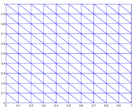
(a) Mesh135, $\alpha_{\text{sum},\mathbb{D}^{-1}}=1.71\pi$           (b) Mesh45, $\alpha_{\text{sum},\mathbb{D}^{-1}}=0.86\pi$

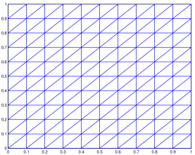
Figure 1: Typical Mesh45 and Mesh135 meshes used in the computation for Example 5.1.

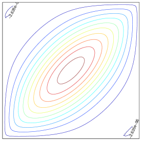
(a) with Mesh135           (b) with Mesh45

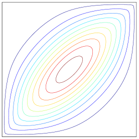
Figure 2: Example 5.1. Contours of the numerical eigenfunctions obtained with $J=81$, where $J$ is the number of mesh points in the $x$ (or $y$) axis.

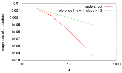
(a) Undershoot with Mesh135           (b) Error in $\lambda_{1}$ with Mesh45 and Mesh135

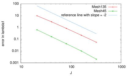
Figure 3: Example 5.1. The magnitude of the undershoot in the computed principal eigenfunction and the error in the computed principal eigenvalue are plotted as function of $J$. In (b), the reference value is $\lambda_{1}\approx 150.288$ which is obtained with a Mesh45 of $J=641$.

      Example 5.2.

The second example is in the form of (1) with

$$\mathbb{D}=\left[\begin{array}[]{rr}10&9\\ 9&10\end{array}\right],\quad\mbox{\boldmath$b$}=\left[\begin{array}[]{c}50\\ -50\end{array}\right],\quad c=1.$$ (30)

Notice that this example is similar to the previous one except that this example contains both the convection and reaction terms and is nonsymmetric. Both Mesh135 and Mesh45 in Fig. 1 are used in the computation.

Recall that Mesh135 does not satisfy the mesh condition (24). The distribution of the first twenty smallest (in modulus) eigenvalues obtained with Mesh135 ($J=41$ and $J=81$) is shown in Fig. 4. One can see that the smallest eigenvalues are actually complex. On the other hand, Mesh45 satisfies (24) when it is sufficiently fine. The distribution of the first twenty smallest eigenvalues obtained with Mesh45 ($J=41$ and $81$) is shown in Fig. 5. It can be seen that the smallest eigenvalue of the discrete problem (4) is real for both cases with $J=41$ and $81$. Moreover, the figure shows that $\text{Re}(\lambda^{h})\geq\lambda_{1}$ at least for the first twenty smallest eigenvalues.

Fig. 6(a) shows the contours of the numerical eigenfunction obtained with Mesh45 $J=81$ and Fig. 6(b) shows the error in the computed principal eigenvalue as function of $J$.

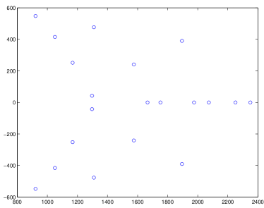
(a) with Mesh135 of $J=41$           (b) with Mesh135 of $J=81$

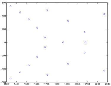
Figure 4: Example 5.2. The distribution of the first twenty smallest (in modulus) eigenvalues for the discrete eigenvalue problem (4) with Mesh135.

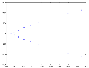
(a) with Mesh45 of $J=41$           (b) with Mesh45 of $J=81$

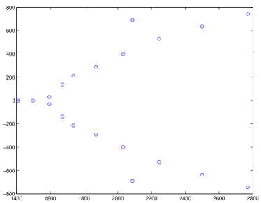
Figure 5: Example 5.2. The distribution of the first twenty smallest (in modulus) eigenvalues for the discrete eigenvalue problem (4) with Mesh45.

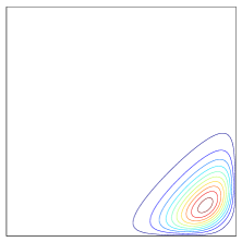
(a) Principal eigenfunction           (b) Error in $\lambda_{1}$ (with the reference value $1401.39$)

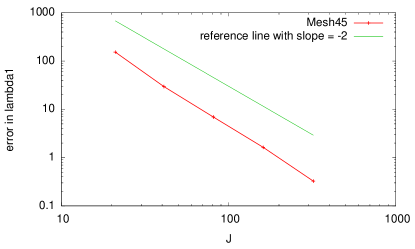
Figure 6: Example 5.2. (a) The contours of the numerical eigenfunction obtained with Mesh45 $J=81$ and (b) the error in the computed principal eigenvalue plotted as function of $J$.

      Example 5.3.

The next example is in the form of (1) with

$$\mathbb{D}=I+0.05\left[\begin{array}[]{cc}\cos(\pi x)&0\\ 0&\sin(\pi y)\end{array}\right],\quad\mbox{\boldmath$b$}=\left[\begin{array}[]{c}20(y-0.5)\\ -20(x-0.5)\end{array}\right],\quad c=1.$$ (31)

Notice that the diffusion matrix and the convection vector are functions of $x$ and $y$. The diffusion matrix is chosen as a small perturbation of the identity matrix so that the acute mesh (in the Euclidean sense) shown in Fig. 7 is also acute in the metric specified by $\mathbb{D}^{-1}$. As a consequence, the mesh condition (23) (and therefore (24)) can be satisfied when the mesh is sufficiently fine.

The contours of a computed principal eigenfunction (with $J=81$) is shown in Fig. 8(a). No undershoot is observed in the solution. The error in $\lambda_{1}$ is plotted in Fig. 8(b) as a function of $J$. The convergence rate is second order.

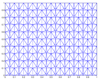
Figure 7: An example ($J=11$) of the mesh used in the computation for Example 5.3 is shown, with $\alpha_{\max,\mathbb{D}^{-1}}=0.49\pi$.

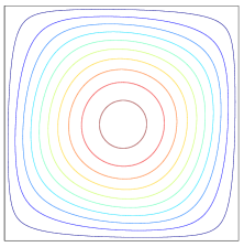
(a) Contours of computed eigenfunction           (b) Error in $\lambda_{1}$ (with the reference value $21.0714$)

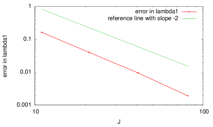
Figure 8: Example 5.3. (a) The contours of the computed principal eigenfunction with $J=81$ and (b) the error in $\lambda_{1}$ plotted as function of $J$.

      Example 5.4.

We have so far considered examples with constant or almost constant diffusion matrices. In this and next examples, we consider the situation with variable diagonal and full diffusion matrices, respectively.

This example is in the form of (1) with

$$\mathbb{D}=\left[\begin{array}[]{cc}100(1-0.5\sin(xy\pi))&0\\ 0&(1+0.5\cos(xy\pi))\end{array}\right],\quad\mbox{\boldmath$b$}=0,\quad c=0.$$ (32)

Since $\mathbb{D}$ changes with location, it is impossible in general to predefine a mesh satisfying the mesh condition (23) or (24). We use here the BAMG (bidimensional anisotropic mesh generator) code developed by Hecht [33] to generate approximate $M$-uniform meshes for the metric tensor $M=\mathbb{D}^{-1}$ (cf. the discussion right after Theorem 4.1). BAMG is a Delaunay-type mesh generator [16] and allows the user to supply a metric tensor defined on a background mesh. It is used in our computation in an iterative fashion: Starting from a coarse mesh, the metric tensor $M=\mathbb{D}^{-1}$ is computed and used in BAMG to generate a new mesh. The process is repeated ten times.

It is noted that $\mathbb{D}$ defined in (32) is diagonal but very anisotropic, with the maximum ratio of the two eigenvalues being over 100. Numerical results show that BAMG is able to generate meshes satisfying (24). Fig. 9(a) shows such a mesh with $\alpha_{\text{sum},\mathbb{D}^{-1}}=0.99\pi$. No undershoot is observed in the computed principal eigenfunctions, as shown in Fig. 10. A second order convergence rate in approximating $\lambda_{1}$ is observed in Fig. 9(b).

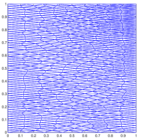
(a) Mesh, $N=1129$, $\alpha_{\text{sum},\mathbb{D}^{-1}}=0.99\pi$           (b) Error in $\lambda_{1}$ (with the reference value $687.666$)

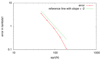
Figure 9: Example 5.4. A typical mesh used in the computation and the convergence history in approximating $\lambda_{1}$.

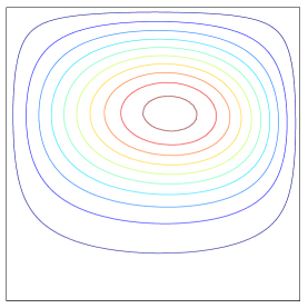
(a) contour plot           (b) surface plot

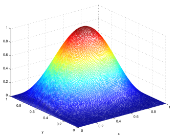
Figure 10: Example 5.4. Contour and surface plots for a computed principal eigenfunction obtained with $N=8925$.

      Example 5.5.

In this final example we consider a full diffusion matrix,

$$\mathbb{D}=\left[\begin{array}[]{cc}\cos(\theta)&-\sin(\theta)\\ \sin(\theta)&\cos(\theta)\end{array}\right]\cdot\left[\begin{array}[]{cc}k(1-0.5\sin(x)\sin(y))&0\\ 0&(1+0.5\cos(x)\cos(y))\end{array}\right]$$ (37)

$$\qquad\qquad\qquad\cdot\left[\begin{array}[]{cc}\cos(\theta)&\sin(\theta)\\ -\sin(\theta)&\cos(\theta)\end{array}\right],$$ (40)

where $k$ is a positive parameter and $\theta=\pi\sin(x)\sin(y)$. We take $\mbox{\boldmath$b$}=0$ and $c=0$ in (1).

We first take $k=10$. BAMG is able to generate meshes satisfying (24) for this case. A mesh and corresponding principal eigenfunction are shown in Fig. 11. Once again, no undershoot is observed. The error in the computed $\lambda_{1}$ is shown in Fig. 13.

Next, we consider a more anisotropic case with $k=100$. For this case, BAMG is not able to produce a mesh satisfying the mesh condition (24). A generated mesh and corresponding principal eigenfunction are plotted in Fig. 12. Interestingly, no undershoot is observed in this case although the stiffness matrix is not an $M$-matrix. This indicates that the $M$-matrix requirement (which is a sufficient requirement in Theorem 3.1) can be replaced with a weaker condition. The error in the computed $\lambda_{1}$ is shown in Fig. 13 to have a second order convergence rate.

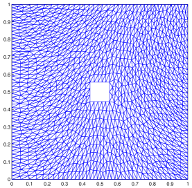
(a) Mesh with $N=2260$, $\alpha_{\text{sum},\mathbb{D}^{-1}}=0.99\pi$           (b) Principal eigenfunction

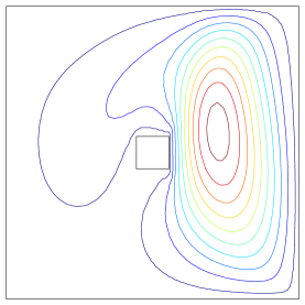
Figure 11: Example 5.5. A typical mesh generated with BAMG for metric tensor $M=\mathbb{D}^{-1}$ ($k=10$) and the corresponding computed principal eigenfunction.

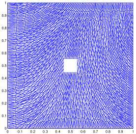
(a) Mesh with $N=2373$, $\alpha_{\text{sum},\mathbb{D}^{-1}}=1.23\pi$           (b) Principal eigenfunction

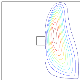
Figure 12: Example 5.5. A typical mesh generated with BAMG for metric tensor $M=\mathbb{D}^{-1}$ ($k=100$) and the corresponding computed principal eigenfunction.

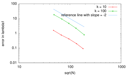
Figure 13: Example 5.5. The error in $\lambda_{1}$ is plotted as function of $\sqrt{N}$, where $N$ is the number of mesh elements. The reference values for $\lambda_{1}$ are 170.422 for $k=10$ and 1020.15 for $k=100$.

6 Conclusions and further comments

In the previous sections we have studied the P1 finite element approximation of the eigenvalue problem of second-order elliptic differential operators subject to the Dirichlet boundary condition. The focus is on the preservation of some basic properties of the principal eigenvalue and eigenfunctions. It has been shown in Theorem 3.1 that if the stiffness matrix is an irreducible $M$-matrix, the algebraic eigenvalue problem resulting from the P1 finite element discretization preserves most basic properties of the principal eigenvalue and eigenfunctions of the continuous problem. These properties include the principal eigenvalue being real and simple and the corresponding eigenfunctions being either positive or negative inside the physical domain. The mesh conditions leading to such a stiffness matrix have been investigated and the main result is stated in Theorem 4.1. Roughly speaking, the theorem states that if the mesh is simplicial, acute (in 2D this condition can be replaced by the Delaunay condition) when measured in the metric specified by the inverse of the diffusion matrix, and interiorly connected, then the stiffness matrix is an irreducible $M$-matrix.

Numerical examples have been presented to verify the theoretical findings. They also show that when the stiffness matrix is not an $M$-matrix, there is no guarantee that the resulting algebraic eigenvalue problem preserve the basic properties of the principal eigenvalue and eigenfunctions. Particularly, the eigenfunctions corresponding to the smallest eigenvalue may change sign and even more, the smallest eigenvalue (in modulus) may not necessarily be real for nonsymmetric operators. Furthermore, numerical results show that those basic properties can be preserved for some non-$M$-matrix situations. This indicates that the $M$-matrix requirement may be weakened. A possibility is to use generalized $M$-matrices [25] although it is not obvious how conditions for generalized $M$-matrices can directly result in mesh conditions that can be used in practical computation. Finally, Example 5.5 shows that it is challenging to generate meshes satisfying the conditions in Theorem 4.1 for a general diffusion matrix. How to generate such meshes deserves more investigations in the future.

Acknowledgment. The work was partially supported by the NSF under grant DMS-1115118. The author would like to thank Weishi Liu, Erik Van Vleck, and Hongguo Xu for useful discussion during the preparation of this work.

References

- [1] D. Ait-Ali-Yahia, G. Baruzzi, W. G. Habashi, M. Fortin, J. Dompierre, and M.-G. Vallet. Anisotropic mesh adaptation: towards user-independent, mesh-independent and solver-independent CFD. Part II: Structured grids. Int. J. Numer. Meth. Fluids, 39:657–673, 2002.
- [2] I. Babuška and J. Osborn. Eigenvalue problems. In Handbook of numerical analysis, Vol. II, Handb. Numer. Anal., II, pages 641–787. North-Holland, Amsterdam, 1991.
- [3] I. Babuška and J. E. Osborn. Finite element-Galerkin approximation of the eigenvalues and eigenvectors of selfadjoint problems. Math. Comp., 52:275–297, 1989.
- [4] A. Berman and R. J. Plemmons. Nonnegative Matrices in the Mathematical Sciences. Society for Industrial and Applied Mathematics, Philadelphia, 1994.
- [5] M. Bern, L. P. Chew, D. Eppstein, and J. Ruppert. Dihedral bounds for mesh generation in high dimensions. In Proc. 6th ACM-SIAM Symp. Discrete Algorithms, pages 89–196, 1995.
- [6] M. Bern, D. Eppstein, and J. Gilbert. Provably good mesh generation. J. Comp. System Sciences, 48:384–409, 1994.
- [7] G. Birkhoff, C. de Boor, B. Swartz, and B. Wendroff. Rayleigh-Ritz approximation by piecewise cubic polynomials. SIAM J. Numer. Anal., 3:188–203, 1966.
- [8] D. Boffi. Finite element approximation of eigenvalue problems. Acta Numer., 19:1–120, 2010.
- [9] D. Boffi, F. Gardini, and L. Gastaldi. Some remarks on eigenvalue approximation by finite elements. In J. Blowey and M. Jensen, editors, Frontiers in Numerical Analysis Durham 2010, volume 85 of Lecture Notes in Computational Science and Engineering, pages 1 – 77, Berlin, Heidelberg, 2010. Springer-Verlag.
- [10] H. Borouchaki, P. L. George, P. Hecht, P. Laug, and E. Saletl. Delaunay mesh generation governed by metric specification: Part I. Algorithms. Fin. Elem. Anal. Des., 25:61–83, 1997.
- [11] H. Borouchaki, P. L. George, and B. Mohammadi. Delaunay mesh generation governed by metric specification: Part II. Applications. Fin. Elem. Anal. Des., 25:85–109, 1997.
- [12] F. J. Bossen and P. S. Heckbert. A pliant method for anisotropic mesh generation. In Proceedings, 5th International Meshing Roundtable, pages 63–74, Sandia National Laboratories, Albuquerque, NM, 1996. Sandia Report 96-2301.
- [13] J. Brandts, S. Korotov, and M. Křížek. The discrete maximum principle for linear simplicial finite element approximations of a reaction-diffusion problem. Lin. Alg. Appl., 429:2344–2357, 2008.
- [14] J. Brandts, S. Korotov, M. Křížek, and J. Šolc. On nonobtuse simplicial partitions. SIAM Rev., 51:317–335, 2009.
- [15] E. Burman and A. Ern. Discrete maximum principle for Galerkin approximations of the Laplace operator on arbitrary meshes. C. R. Acad. Sci. Paris, Ser.I 338:641–646, 2004.
- [16] M. J. Castro-Díaz, F. Hecht, B. Mohammadi, and O. Pironneau. Anisotropic unstructured mesh adaption for flow simulations. Int. J. Numer. Meth. Fluids, 25:475–491, 1997.
- [17] P. G. Ciarlet. Discrete maximum principle for finite difference operators. Aequationes Math., 4:338–352, 1970.
- [18] P. G. Ciarlet. The Finite Element Method for Elliptic Problems. North-Holland, Amsterdam, 1978.
- [19] P. G. Ciarlet and P.-A. Raviart. Maximum principle and uniform convergence for the finite element method. Comput. Meth. Appl. Mech. Engrg., 2:17–31, 1973.
- [20] X. Dai, J. Xu, and A. Zhou. Convergence and optimal complexity of adaptive finite element eigenvalue computations. Numer. Math., 110:313–355, 2008.
- [21] X. Dai and A. Zhou. Three-scale finite element discretizations for quantum eigenvalue problems. SIAM J. Numer. Anal., 46:295–324, 2007/08.
- [22] M. de Berg, M. van Kreveld, M. Overmars, and O. Schwarzkopf. Computational Geometry. Springer, Berlin, 2000.
- [23] J. Dompierre, M.-G. Vallet, Y. Bourgault, M. Fortin, and W. G. Habashi. Anisotropic mesh adaptation: towards user-independent, mesh-independent and solver-independent CFD. Part III: Unstructured meshes. Int. J. Numer. Meth. Fluids, 39:675–702, 2002.
- [24] A. Drǎgǎnescu, T. F. Dupont, and L. R. Scott. Failure of the discrete maximum principle for an elliptic finite element problem. Math. Comp., 74:1–23, 2004.
- [25] A. Elhashash and D. B. Szyld. Generalizations of -matrices which may not have a nonnegative inverses. Lin. Alg. Appl., 429:2435 – 2450, 2008.
- [26] D. Eppstein, J. M. Sullivan, and A. Ungor. Tiling space and slabs with acute tetrahedra. Comput. Geom. Theory & Appl., 27:237–255, 2004.
- [27] L. C. Evans. Partial Differential Equations. American Mathematical Society, Providence, Rhode Island, 1998. Graduate Studies in Mathematics, Volume 19.
- [28] G. J. Fix. Eigenvalue approximation by the finite element method. Advances in Math., 10:300–316, 1973.
- [29] R. V. Garimella and M. S. Shephard. Boundary layer meshing for viscous flows in complex domain. In Proceedings, 7th International Meshing Roundtable, pages 107–118, Sandia National Laboratories, Albuquerque, NM, 1998.
- [30] S. Gűnter and K. Lackner. A mixed implicit-explicit finite difference scheme for heat transport in magnetised plasmas. J. Comput. Phys., 228:282–293, 2009.
- [31] S. Gűnter, Q. Yu, J. Kruger, and K. Lackner. Modelling of heat transport in magnetised plasmas using non-aligned coordinates. J. Comput. Phys., 209:354–370, 2005.
- [32] W. G. Habashi, J. Dompierre, Y. Bourgault, D. Ait-Ali-Yahia, M. Fortin, and M.-G. Vallet. Anisotropic mesh adaptation: towards user-independent, mesh-independent and solver-independent CFD. Part I: General principles. Int. J. Numer. Meth. Fluids, 32:725–744, 2000.
- [33] F. Hecht. BAMG – Bidimensional Anisotropic Mesh Generator homepage. http://www.ann.jussieu.fr/hecht/ftp/bamg/, 1997.
- [34] R. A. Horn and C. A. Johnson. Matrix Analysis. Cambridge University Press, Cambridge, London, 1985.
- [35] J. Hu, Y. Huang, and Q. Lin. Lower bounds for eigenvalues of elliptic operators – by nonconforming finite element methods. 2012. (arXiv: 1112.1145).
- [36] W. Huang. Variational mesh adaptation: isotropy and equidistribution. J. Comput. Phys., 174:903–924, 2001.
- [37] W. Huang. Mathematical principles of anisotropic mesh adaptation. Comm. Comput. Phys., 1:276–310, 2006.
- [38] W. Huang. Discrete maximum principle and a delaunay-type mesh condition for linear finite element approximations of two-dimensional anisotropic diffusion problems. Numer. Math. Theory Meth. Appl., 4:319–334, 2011. (arXiv:1008.0562).
- [39] W. Huang and R. D. Russell. Adaptive Moving Mesh Methods. Springer, New York, 2011. Applied Mathematical Sciences Series, Vol. 174.
- [40] J. Karátson and S. Korotov. An algebraic discrete maximum principle in Hilbert space with applications to nonlinear cooperative elliptic systems. SIAM J. Numer. Anal., 47:2518–2549, 2009.
- [41] J. Karátson, S. Korotov, and M. Křížek. On discrete maximum principles for nonlinear elliptic problems. Math. Comput. Sim., 76:99–108, 2007.
- [42] D. Kuzmin, M. J. Shashkov, and D. Svyatskiy. A constrained finite element method satisfying the discrete maximum principle for anisotropic diffusion problems. J. Comput. Phys., 228:3448–3463, 2009.
- [43] M. Křížek and Q. Lin. On diagonal dominance of stiffness matrices in 3D. East-West J. Numer. Math., 3:59–69, 1995.
- [44] C. Le Potier. A nonlinear finite volume scheme satisfying maximum and minimum principles for diffusion operators. Int. J. Finite Vol., 6:20 pp., 2009.
- [45] F. W. Letniowski. Three-dimensional Delaunay triangulations for finite element approximations to a second-order diffusion operator. SIAM J. Sci. Stat. Comput., 13:765–770, 1992.
- [46] X. P. Li and W. Huang. An anisotropic mesh adaptation method for the finite element solution of heterogeneous anisotropic diffusion problems. J. Comput. Phys., 229:8072–8094, 2010 (arXiv:1003.4530v2).
- [47] X. P. Li, D. Svyatskiy, and M. Shashkov. Mesh adaptation and discrete maximum principle for 2D anisotropic diffusion problems. Technical Report LA-UR 10-01227, Los Alamos National Laboratory, Los Alamos, NM, 2007.
- [48] K. Lipnikov, M. Shashkov, D. Svyatskiy, and Y. Vassilevski. Monotone finite volume schemes for diffusion equations on unstructured triangular and shape-regular polygonal meshes. J. Comput. Phys., 227:492–512, 2007.
- [49] R. Liska and M. Shashkov. Enforcing the discrete maximum principle for linear finite element solutions of second-order elliptic problems. Comm. Comput. Phys., 3:852–877, 2008.
- [50] C. Lu, W. Huang, and J. Qiu. Maximum principle in linear finite element approximations of anisotropic diffusion-convection-reaction problems. 2012. (arXiv:1201.3651).
- [51] F. Luo, Q. Lin, and H. Xie. Computing the lower and upper bounds of Laplace eigenvalue problem: by combining conforming and nonconforming finite element methods. Sci. China Math., 55:1069–1082, 2012.
- [52] V. Mehrmann and A. Miedlar. Adaptive computation of smallest eigenvalues of self-adjoint elliptic partial differential equations. Numer. Lin. Alg. Appl., 18:387–409, 2011.
- [53] M. J. Mlacnik and L. J. Durlofsky. Unstructured grid optimization for improved monotonicity of discrete solutions of elliptic equations with highly anisotropic coefficients. J. Comput. Phys., 216:337–361, 2006.
- [54] A. Naga and Z. Zhang. Function value recovery and its application in eigenvalue problems. SIAM J. Numer. Anal., 50:272–286, 2012.
- [55] J. Peraire, M. Vahdati, K. Morgan, and O. C. Zienkiewicz. Adaptive remeshing for compressible flow computations. J. Comput. Phy., 72:449 – 466, 1997.
- [56] J.-F. Remacle, X. Li, M. S. Shephard, and J. E. Flaherty. Anisotropic adaptive simulation of transient flows using discontinuous Galerkin methods. Int. J. Numer. Methods Engrg., 62:899–923, 2005.
- [57] P. Sharma and G. W. Hammett. Preserving monotonicity in anisotropic diffusion. J. Comput. Phys., 227:123–142, 2007.
- [58] Z. Sheng and G. Yuan. The finite volume scheme preserving extremum principle for diffusion equations on polygonal meshes. J. Comput. Phys., 230:2588–2604, 2011.
- [59] G. Stoyan. On maximum principles for monotone matrices. Lin. Alg. Appl., 78:147–161, 1986.
- [60] G. Strang and G. J. Fix. An Analysis of the Finite Element Method. Prentice Hall, Englewood Cliffs, NJ, 1973.
- [61] J. Wang and R. Zhang. Maximum principle for P1-conforming finite element approximations of quasi-linear second order elliptic equations. SIAM J. Numer. Anal., 50:626–642, 2012. (arXiv:1105.1466).
- [62] J. Xu and A. Zhou. A two-grid discretization scheme for eigenvalue problems. Math. Comp., 70:17–25, 2001.
- [63] J. Xu and L. Zikatanov. A monotone finite element scheme for convection-diffusion equations. Math. Comput., 69:1429–1446, 1999.
- [64] S. Yamakawa and K. Shimada. High quality anisotropic tetrahedral mesh generation via ellipsoidal bubble packing. In Proceedings, 9th International Meshing Roundtable, pages 263–273, Sandia National Laboratories, Albuquerque, NM, 2000. Sandia Report 2000-2207.
- [65] Y. Yang and H. Bi. Two-grid finite element discretization schemes based on shifted-inverse power method for elliptic eigenvalue problems. SIAM J. Numer. Anal., 49:1602–1624, 2011.
- [66] Y. Yang, Z. Zhang, and F. Lin. Eigenvalue approximation from below using non-conforming finite elements. Sci. China Math., 53:137–150, 2010.
- [67] G. Yuan and Z. Sheng. Monotone finite volume schemes for diffusion equations on polygonal meshes. J. Comput. Phys., 227:6288–6312, 2008.
- [68] Y. Zhang, X. Zhang, and C.-W. Shu. Maximum-principle-satisfying second order discontinuous Galerkin schemes for convection-diffusion equations on triangular meshes. J. Comput. Phys., 234:295 – 316, 2013.