Phase space flow in the Husimi representation

Abstract

We derive a continuity equation for the Husimi function evolving under a general non-hermitian Hamiltonian and identify the phase space flow associated with it. For the case of unitary evolution we obtain explicit formulas for the quantum flow, which can be written as a classical part plus semiclassical corrections. These equations are the analogue of the Wigner flow, which displays several non-intuitive features like momentum inversion and motion of stagnation points. Many of these features also appear in the Husimi flow and, therefore, are not related to the negativity of the Wigner function as previously suggested. We test the exact and semiclassical formulas for a particle in a double well potential. We find that the zeros of the Husimi function are saddle points of the flow, and are always followed by a center. Merging or splitting of stagnation points, observed in the Wigner flow, does not occur because of the isolation of the Husimi zeros.

I Introduction

In classical mechanics the state of a system is often associated to a point in phase space. The initial condition defined by this point specifies a unique trajectory that guides the evolution of the system. This association, however, is not accurate in many situations due to imprecisions in assessing the system’s state or the statistical nature of the problem at hand. In these cases it is better to work with probability distributions and the associated Liouville equation than with individual trajectories and Hamilton’s equations.

In one-dimension the phase space is constructed with a pair of canonically conjugate variables, position $x$ and momentum $p$, and the classical dynamics of a function $F\left(x,p;t\right)$ can be written in the form of a continuity equation

$$\frac{\partial F}{\partial t}+\mathbf{\nabla\cdot J}_{cl}=0$$ (1)

where $\mathbf{\nabla}=\left(\frac{\partial}{\partial x},\frac{\partial}{\partial p}\right)$, the classical current vector is given by

$$\mathbf{J}_{cl}=\left(\begin{array}[]{c}J_{x}\\ J_{p}\end{array}\right)=\left(\begin{array}[]{c}\dot{x}F\\ \dot{p}F\end{array}\right),$$ (2)

and the dots indicate total derivative with respect to time. The characteristic property of this construction is that each point of the phase space on which $F$ is evaluated is guided by a well-defined trajectory and the flow lines of the current are just the tangent vectors to these trajectories. The dynamics of the function $F$ is thus trivial in the sense that the points just follow the flow, that is, $F\left(x,p;t\right)=F\left(x_{0},p_{0};0\right)$ where $x_{0}$ and $p_{0}$ are the initial conditions that propagate to $x$ and $p$ in the time $t$.

In quantum mechanics states are naturally described in terms of probability distributions but, due to the uncertainty principle, phase space representations have interpretations that are different from their classical counterparts. Two of the most used quantum phase space representations are the Wigner and the Husimi functions. The Wigner function $W(x,p,t)$ associated to a pure state $|\psi\rangle$ has the correct marginal probability distributions when projected into the $x$ or $p$ subspaces, but can be itself negative. The Husimi distribution $Q\left(x,p,t\right)$, on the other hand, is positive by definition, but does not project onto the correct marginal distributions. Despite these well known properties, both representations, and others as well, have been successful employed in many quantum mechanical treatments glauber ; cohen ; hillery ; kla ; perel , particularly in the study of the boundary between quantum and classical mechanics hell75 ; hk84 ; berry89 ; kurchan89 ; xavier97 ; kay94a ; kay94b ; ozorio98 ; bar01 ; mill01 ; pollak03 ; rib04 ; sha04 ; sha08 ; agui10 ; thiago11a ; thiago11b .

If $F(x,p;t)$ is a phase space representation of a quantum state, a natural question to ask is whether it obeys a continuity equation similar to (1) and if a flow can be defined. The difficulty resides in the uncertainty principle, that forbids the definition of authentic quantum trajectories $x\left(t\right)$ and $p\left(t\right)$ guiding the dynamics in these representations. Although it may seem conflicting, it has been previously shown that the dynamics of the Wigner function can indeed be cast as a continuity-like equation donoso03 ; bauke11 ; skr13 , thus confirming that for this particular representation a flow is well-defined even though the trajectories in the classical sense are not.

The quantum flow associated with the Wigner function exhibits many interesting non-classical features, like travelling stagnation points that can merge with or split from other such points, vortices and conservation of the flow winding number skr13 . It was argued that many of these complex features were consequences of the negativity of the Wigner function.

In this work we employ the coherent state representation and develop a flow formalism for the Husimi function. A continuity equation for the Husimi dynamics has already been demonstrated but only for a particular class of systems skodje89 . Here we derive formulas for the Husimi flow for very general Hamiltonian systems and compare features of this flow with those of the Wigner function.

We show that for Hermitian Hamiltonians there are no source or sink terms, which do appear for non-unitary evolution. Like its Wigner counterpart, non-local features lead to noticeable time-dependent distortions with respect to the classical flow lines, including the displacement and motion of the classical stability points and inversion of momentum. In skr13 it was reasoned that inversion of momentum lines of the flow for the Wigner function was caused by negativity of the function, which is itself a mark of non-classicality. The inversion of momentum lines was also found here, for a positive definite function, implying that such inversions are a more robust sign of quantumness than negativity for some particular representation. For the considered example we also found that every zero of the Husimi function behaves as a saddle point of the currents, with no other saddles identified beside these zeros.

The paper is organized as follows: in section II we define the Husimi function and construct the associated continuity equation for general non-Hermitian Hamiltonians. We provide a detailed derivation of the flow and then restrict the calculations to the unitary case. In section III we show how to obtain the classical equation of motion given in terms of Poisson brackets from the quantum flow and also derive semiclassical corrections to the classical flow. In section IV we illustrate these features using as example a one-dimensional double well potential. In section V we make some final remarks about the main results.

II The Husimi flow

II.1 The Husimi function

The coherent states of a harmonic oscillator with mass $m$ and frequency $\Omega$ are defined as the eigenstates of the annihilation operator $\widehat{a}=\left(\gamma\widehat{x}+i\widehat{p}/\gamma\right)/\sqrt{2\hbar}$, where $\gamma=\sqrt{m\Omega}$:

$$\widehat{a}|z\rangle=z|z\rangle.$$ (3)

The normalized coherent states can also be written as

$$|z\rangle=e^{-\frac{1}{2}\left|z\right|^{2}}e^{z\widehat{a}^{\dagger}}|0\rangle,$$ (4)

which will be useful in what follows. Here $|0\rangle$ is the ground state of the oscillator, which is also the coherent state labeled by $z=0$. The eigenvalue $z$ is generally complex and defines a one-dimensional complex manifold $\Xi_{z}$ with volume element $\text{d}^{2}z\equiv\text{d}z^{\star}\wedge\text{d}z/2\pi i$ kla . These states form a basis and

$$\widehat{1}=\int\text{d}^{2}z|z\rangle\langle z|.$$ (5)

The coherent states can also be described as the ground state displaced by a complex amount $z$ in the eigenvalue manifold $\Xi_{z}$. The ground state $|0\rangle$ is a minimum uncertainty gaussian wavepacket in both momentum and position representation, and so are the displaced states $|z\rangle$ perel . The relation between $z$ and the mean momentum $p$ and position $x$ of the displaced state is given by

$$z=\frac{1}{\sqrt{2\hbar}}\left(\gamma x+\frac{ip}{\gamma}\right).$$ (6)

This expression provides a bijection from the classical phase space $\Xi_{cl}$ of the variables $x$ and $p$ to the complex manifold $\Xi_{z}$ which parametrize the set of states $|z\rangle$.

Given a pure one-particle quantum state $|\psi\rangle$ and its projection $\psi\left(z^{\star},z\right)=\langle z|\psi\rangle$, the Husimi function is the quasi-probability density associated to this wavefunction under the volume form $\text{d}^{2}z$:

$$Q_{\psi}\left(z^{\star},z\right)=\left|\psi\left(z^{\star},z\right)\right|^{2}=\text{tr}\left(|z\rangle\langle z|\widehat{\rho}\right)$$ (7)

where $\widehat{\rho}=|\psi\rangle\langle\psi|$ is the density matrix. This function is also called the $Q$-representation or $Q$-symbol of the quantum state. The Husimi function is a positive function over the manifold $\Xi_{z}$, but it is not a probability distribution, since the coordinate and momentum probability densities cannot be retrieved as the marginals distributions from Eq. (7).

II.2 Time dependent states

Consider a time dependent quantum state $|\psi;t\rangle$ evolved under the action of a time independent hamiltonian $\widehat{H}$ (which we do not assume hermitian at this point),

$$|\psi;t\rangle=\widehat{K}\left(t-t_{0}\right)|\psi;t_{0}\rangle,$$

where $\widehat{K}=e^{-i\widehat{H}t/\hbar}$ is the time evolution operator. The Husimi function inherits the time dependence of the state

$$Q_{\psi}\left(z^{\star},z;t\right)=\text{tr}\left(|z\rangle\langle z|\widehat{\rho}\left(t\right)\right),$$ (8)

where $\widehat{\rho}\left(t\right)=|\psi;t\rangle\langle\psi;t|$, and the equation governing the dynamics of the Husimi function becomes

$$i\hbar\frac{\partial}{\partial t}Q_{\psi}=\text{tr}\left(|z\rangle\langle z|\widehat{H}\widehat{\rho}-\widehat{\rho}\widehat{H}^{\dagger}|z\rangle\langle z|\right).$$ (9)

For hermitian Hamiltonians this is just von Neumann’s relation cast in the Husimi representation: $i\hbar\frac{\partial}{\partial t}Q_{\psi}=\text{tr}\left(|z\rangle\langle z|\left[\widehat{H},\widehat{\rho}\right]\right)$. To further simplify this expression we assume that the Hamiltonian can be expressed as a normal ordered power series on the creation and annihilation operators as

$$\widehat{H}=\sum_{m,n}h_{mn}\widehat{a}^{\dagger m}\widehat{a}^{n}.$$ (10)

If $h_{mn}=h_{nm}^{\star}$ the Hamiltonian is hermitian. The normalized matrix elements of the Hamiltonian in the coherent states representation become

$$H\left(z^{\prime\star},z\right)=\frac{\langle z^{\prime}|\widehat{H}|z\rangle}{\langle z^{\prime}|z\rangle}=\sum_{m,n}h_{mn}z^{\prime\star m}z^{n}.$$ (11)

The action of the operators $\widehat{a}^{\dagger}$ and $\widehat{a}$ on the projector $|z\rangle\langle z|$ is given by its differential algebra on the representation of the coherent states gilmore75 ; zhang90 ; trimborn08 and can be derived by appling them to the states as defined in equation (4). For the action to the right the following relations hold:

$$\widehat{a}|z\rangle\langle z| = z|z\rangle\langle z|,$$

$$\widehat{a}^{\dagger}|z\rangle\langle z| = \left(\frac{\partial}{\partial z}+z^{\star}\right)|z\rangle\langle z|.$$

The action of a general term of the Hamiltonian is given as

$$\widehat{a}^{\dagger i}\widehat{a}^{j}|z\rangle\langle z|=z^{j}\left(\frac{\partial}{\partial z}+z^{\star}\right)^{i}|z\rangle\langle z|.$$ (12)

The action to the left is given by analogous relations,

$$|z\rangle\langle z|\widehat{a} = |z\rangle\langle z|\left(\frac{\overleftarrow{\partial}}{\partial z^{\star}}+z\right),$$

$$|z\rangle\langle z|\widehat{a}^{\dagger} = |z\rangle\langle z|z^{\star},$$

leading to

$$|z\rangle\langle z|\widehat{a}^{\dagger j}\widehat{a}^{i}=|z\rangle\langle z|\left(\frac{\overleftarrow{\partial}}{\partial z^{\star}}+z\right)^{i}z^{\star j},$$ (13)

which is just the hermitian transpose of (12) in matrix notation. Eqs. (12) and (13) can be used in Eq.(9) describing the dynamics of the Husimi function. Evaluating the first term inside the trace, using the Hamiltonian power series (10) leads to

$$\text{tr}\left(|z\rangle\langle z|\widehat{H}\widehat{\rho}\right) = \text{tr}\left(|z\rangle\langle z|\sum_{m,n}h_{mn}\widehat{a}^{\dagger m}\widehat{a}^{n}\widehat{\rho}\right)$$

$$= \text{tr}\left(|z\rangle\langle z|\widehat{\rho}\right)\sum_{m,n}h_{mn}\left[\left(\frac{\overleftarrow{\partial}}{\partial z^{\star}}+z\right)^{n}z^{\star m}\right]$$

$$= \sum_{m,n}h_{mn}z^{\star m}\left(\frac{\partial}{\partial z^{\star}}+z\right)^{n}Q_{\psi}.$$

The passing from the first to the second line can be accomplished by the linearity of the trace, and from the second to the third line a rearrangement of the factors was performed, putting the derivative operator acting to the right as usual. A similar calculation can be done for the second term inside the trace in Eq.(9). The resulting equation is

$$i\hbar\frac{\partial}{\partial t}Q_{\psi}=\sum_{m,n}h_{mn}z^{\star m}\left(\frac{\partial}{\partial z^{\star}}+z\right)^{n}Q_{\psi}-\sum_{m,n}h_{mn}^{\star}z^{m}\left(\frac{\partial}{\partial z}+z^{\star}\right)^{n}Q_{\psi}.$$ (14)

Since the Husimi is a real function, $\frac{\partial}{\partial z^{\star}}Q_{\psi}=\left(\frac{\partial}{\partial z}Q_{\psi}\right)^{\star}$. Therefore, although the dynamical equation for $Q_{\psi}$ is the sum of two complex functions, its time evolution remains real as it should.

II.3 Continuity equation and Flow

In order to write the equation (14) as a continuity equation all the derivatives with respect to $z^{\star}$ and $z$ must be put to the left, so that we can single out terms of the form $\frac{\partial}{\partial z}J_{z}$ and $\frac{\partial}{\partial z^{\star}}J_{z^{\star}}$, identifying in this way the Husimi currents $J_{z}$ and $J_{z^{\star}}$. The relation between these complex currents in $\Xi_{z}$ and the real ones in the classical phase space $\Xi_{cl}$ (2) can be obtained employing the following transformation law for the derivatives in $\Xi_{z}$ and $\Xi_{cl}$:

$$\begin{gathered}\frac{\partial}{\partial z}=\frac{\sqrt{\hbar/2}}{\gamma}\frac{\partial}{\partial x}-i\gamma\sqrt{\hbar/2}\frac{\partial}{\partial p},\\ \frac{\partial}{\partial z^{\star}}=\frac{\sqrt{\hbar/2}}{\gamma}\frac{\partial}{\partial x}+i\gamma\sqrt{\hbar/2}\frac{\partial}{\partial p}.\end{gathered}$$ (15)

We obtain

$$J_{x}=\frac{\sqrt{\hbar/2}}{\gamma}\left(J_{z^{\star}}+J_{z}\right),\qquad J_{p}=i\gamma\sqrt{\hbar/2}\left(J_{z^{\star}}-J_{z}\right).$$ (16)

To put derivatives to the left in (14), we need to change the position of the terms $\left(\frac{\partial}{\partial z^{\star}}+z\right)^{j}$ and $\left(\frac{\partial}{\partial z}+z^{\star}\right)^{j}$ with that of the terms $z^{\star i}$ and $z^{i}$, respectively. A concise way to express both changes is to define

$$\begin{cases}X=z^{\star}&\text{and }D=\left(\frac{\partial}{\partial z^{\star}}+z\right)\\ &\text{or}\\ X=z&\text{and }D=\left(\frac{\partial}{\partial z}+z^{\star}\right).\end{cases}$$

In both cases, $XD=DX-1$, and we need to express the $X^{i}D^{j}$ term as a combination of those with the opposite ordering. This calculation can be done by induction and the swapping of factors results

$$X^{i}D^{j}=\sum_{k=0}^{\min\left(i,j\right)}r_{i,j,k}D^{j-k}X^{i-k},$$

where

$$r_{i,j,k}=\frac{\left(-1\right)^{k}i!j!}{k!\left(i-k\right)!\left(j-k\right)!}.$$

Substituting the series above for the commutation of derivatives and functions in Eq.(14) and expanding the binomials inside the definition of $D$, we end up with

$$\frac{\partial}{\partial t}Q_{\psi}=\frac{1}{i\hbar}\sum_{m,n}\sum_{k=0}^{\min\left(m,n\right)}\sum_{l=0}^{n-k}h_{mn}r_{m,n,k}\binom{n-k}{l}\frac{\partial^{l}}{\partial z^{\star l}}z^{n-k-l}z^{\star m-k}Q_{\psi}+\\ -\frac{1}{i\hbar}\sum_{m,n}\sum_{k=0}^{\min\left(m,n\right)}\sum_{l=0}^{n-k}h_{mn}^{\star}r_{m,n,k}\binom{n-k}{l}\frac{\partial^{l}}{\partial z^{l}}z^{\star n-k-l}z^{m-k}Q_{\psi}.$$ (17)

Before we factor out the derivatives identifying the currents we notice that in each summation there is a collection of terms having no derivatives at all, that is, $l=0$. These terms play the role of a source contribution $\sigma$ to the continuity equation. The explicit expression for this source is

$$\sigma=\frac{1}{i\hbar}\sum_{m,n}\sum_{k=0}^{\min\left(m,n\right)}r_{m,n,k}\left(h_{mn}z^{n-k}z^{\star m-k}-\text{c.c.}\right)Q_{\psi},$$

where c.c. stands for complex conjugate. If the Hamiltonian is hermitian it can be shown, using the fact that the coefficients $r_{i,j,k}$ are symmetric in the $i$ and $j$ indexes, that the source vanishes, which is expected for the unitary evolution.

From now on we assume that the Hamiltonian is hermitian and drop off the source terms. Taking out to the left one derivative of the expression (17) we can write at last

$$\frac{\partial}{\partial t}Q_{\psi}=-\frac{\partial}{\partial z}J_{z}-\frac{\partial}{\partial z^{\star}}J_{z^{\star}},$$ (18)

where the currents are given by

$$J_{z} = \frac{1}{i\hbar}\sum_{m,n}\sum_{k=0}^{\min\left(m,n\right)}\sum_{l=1}^{n-k}h_{nm}r_{m,n,k}\binom{n-k}{l}\frac{\partial^{l-1}}{\partial z^{l-1}}z^{\star n-k-l}z^{m-k}Q_{\psi},$$ (19)

$$J_{z^{\star}} = -\frac{1}{i\hbar}\sum_{m,n}\sum_{k=0}^{\min\left(m,n\right)}\sum_{l=1}^{n-k}h_{mn}r_{m,n,k}\binom{n-k}{l}\frac{\partial^{l-1}}{\partial z^{\star l-1}}z^{n-k-l}z^{\star m-k}Q_{\psi}.$$ (20)

It can be readily checked that $J_{z^{\star}}=J_{z}^{\star}$, such that our expectation about having real currents (16) on $\Xi_{cl}$ are met and the following relations stand

$$J_{x}=\frac{\sqrt{2\hbar}}{\gamma}\text{Re}\left(J_{z}\right),\qquad J_{p}=\gamma\sqrt{2\hbar}\text{Im}\left(J_{z}\right).$$

As remarked before, these currents do define a flow on the phase space, and this flow has a crucial dependence on the shape of the Husimi function, rendered by the high order derivatives appearing in Eqs.(19) and (20), coupled to the zero point Taylor coefficients of the Hamiltonian itself. This dependence shows that the coupling in phase space does not have a local character, thus being a fingerprint of nonlocality in this construction.

III Classical limit and Semiclassical corrections

III.1 Classical currents

In the limit $\hbar\rightarrow 0$ the currents given by Eqs. (19) and (20) should reduce to the classical Liouville currents Eq.(2). A complication that arises in the investigation of this limit is that the Hamiltonian function $H\left(z^{\prime\star},z\right)$ itself involves terms of order $\hbar$ or higher coming from the normal ordering process, and nothing precludes the Husimi function $Q_{\psi}\left(z^{\star},z\right)$ of such $\hbar$ dependence as well. A true expansion of the equations in powers of $\hbar$ might take these terms into account order by order. To avoid this extra difficulty we will always take the full Hamiltonian $H\left(z^{\prime\star},z\right)$ and the full Husimi function $Q_{\psi}\left(z^{\star},z\right)$ into account and expand only the dynamical equation for the flow. Thus, each order will contain some higher order terms in $\hbar$ coming only from the Hamiltonian and the Husimi function. As an example consider

$$\widehat{H}=\frac{\widehat{p}^{2}}{2m}-\frac{k}{2}\widehat{x}^{2}+\lambda\widehat{x}^{4}+V_{0}$$ (21)

for which we find

$$H = -\frac{\hbar\Omega}{4}(z-z^{\star})^{2}-\frac{k\hbar}{4m\Omega}(z+z^{\star})^{2}+\frac{\lambda\hbar^{2}}{4m^{2}\Omega^{2}}(z+z^{\star})^{4}+V_{0}$$ (23)

$$+\frac{\hbar\Omega}{4}-\frac{k\hbar}{4m\Omega}+\frac{3\hbar^{2}\lambda}{4m^{2}\Omega^{2}}+\frac{3\hbar^{2}\lambda}{2m^{2}\Omega^{2}}(z+z^{\star})^{2}.$$

In equation (6) we factored out the $\hbar$ dependence of the phase space variables $z$ and $z^{\star}$, which makes them proportional to $\hbar^{-1/2}$. The derivatives $\partial/\partial z$ and $\partial/\partial z^{\star}$, in turn, are proportional to $\hbar^{1/2}$. In terms of $x$ and $p$, we obtain

$$\tilde{H} = \frac{p^{2}}{2m}-\frac{kx^{2}}{2}+\lambda x^{4}+V_{0}$$ (25)

$$+\frac{\hbar\Omega}{4}-\frac{\hbar k}{4m\Omega}+\frac{3\hbar\lambda x^{2}}{m\Omega}+\frac{3\hbar^{2}\lambda}{4m^{2}\Omega^{2}}$$

where the tilde identifies the functions written in the $\Xi_{cl}$ variables $x$ and $p$.

In both these expressions, the first line corresponds to the classical Hamiltonian and is $\hbar$ independent. The second lines contain the corrections. It is therefore clear that if the quantum Hamiltonian operator is independent of $\hbar$, each monomial $h_{mn}z^{\star m}z^{n}$ is of order $\hbar^{0}$ plus corrections coming from normal ordering the creation and annihilation operators.

In what follows we investigate the semiclassical limit without expanding the Hamiltonian and the Husimi function. Although such complete expansion could be performed, it is much more complicated and does not bring any insight into the structure of the flow. Using this scheme, the classical limit becomes

$$\lim_{\hbar\rightarrow 0}J_{z}=\lim_{\hbar\rightarrow 0}\sum_{q=0}^{q_{max}}\hbar^{q}j_{q}\left(z^{\star},z;t\right)=j_{0}\left(z^{\star},z;t\right),$$

with all terms $h_{mn}z^{\star m}z^{n}$ treated as $\hbar^{0}$. Here $q_{max}$ as the highest power of $\hbar$ in such expansion. In order to connect $q$ with the indexes $m$, $n$, $k$ and $l$ present in the summation formulae for the currents we write Eq.(19) as

$$J_{z}=i\sum_{m,n}\sum_{k=0}^{\min\left(m,n\right)}\sum_{l=1}^{n-k}\hbar^{k+l-1}f_{m,n,k,l},$$

set $q=k+l-1$ and identify $j_{q}$ with the proper summation over a set of the $f_{m,n,k,l}$ (see below). For hermitian Hamiltonians whose highest power in the annihilation and creation operators is $n_{max}$, we find $q_{max}=n_{max}-1$

To analyze the general term with a given $\hbar$ power $q$ in Eq.(19), we replace the $l$ by $l=q-k+1$, with $k\leq q\leq n-1$, whenever $k\leq n-1$:

$$J_{z}=\frac{1}{i\hbar}\sum_{m,n}\sum_{k=0}^{\min\left(m,n-1\right)}\sum_{q=k}^{n-1}h_{nm}r_{m,n,k}\binom{n-k}{q-k+1}\frac{\partial^{q-k}}{\partial z^{q-k}}z^{\star n-q-1}z^{m-k}Q_{\psi}.$$ (26)

A similar expression holds for $J_{z^{\star}}$. Now the $\hbar\rightarrow 0$ limit can be taken by selecting the term $q=k=0$ in this summation. The result is

$$J_{z}=\frac{1}{i\hbar}\sum_{m,n}nh_{nm}z^{\star n-1}z^{m}Q_{\psi}=\frac{1}{i\hbar}\frac{\partial H}{\partial z^{\star}}Q_{\psi},$$ (27)

where $H\equiv H\left(z^{\star},z\right)$, as defined in (11), does contain higher powers of $\hbar$ as discussed above, as the Husimi function. Analogously,

$$J_{z^{\star}}=-\frac{1}{i\hbar}\frac{\partial H}{\partial z}Q_{\psi}.$$ (28)

The classical currents, calculated from (27) and (28) are given by

$$J_{x}=\frac{\partial\tilde{H}}{\partial p}\tilde{Q}_{\psi},\qquad J_{p}=-\frac{\partial\tilde{H}}{\partial x}\tilde{Q}_{\psi}.$$ (29)

By direct comparison of equations (2) and (29) we can extract the classical equations of motion in the phase space

$$\dot{x}=\frac{\partial\tilde{H}}{\partial p},\qquad\dot{p}=-\frac{\partial\tilde{H}}{\partial x}.$$

Notice that we have not made any assumptions regarding trajectories being guided by a Hamiltonian. The classical structure emerges naturally from the quantum case. Going a step further, the dynamics of the Husimi function in the classical limit is governed by the equation

$$\frac{\partial}{\partial t}\tilde{Q}_{\psi} = -\frac{\partial}{\partial x}\left(\frac{\partial\tilde{H}}{\partial p}\tilde{Q}_{\psi}\right)-\frac{\partial}{\partial p}\left(-\frac{\partial\tilde{H}}{\partial x}\tilde{Q}_{\psi}\right)$$

$$= \left\{\tilde{H},\tilde{Q}_{\psi}\right\}_{\left[x,p\right]},$$

where $\left\{\cdot,\cdot\right\}_{\left[x,p\right]}$ is the Poisson bracket in the coordinates $x$ and $p$. The additional terms, in higher order of $\hbar$, in Eq.(26) lead to quantum deviations from the classical flow.

III.2 Semiclassical corrections

The first quantum corrections to the classical dynamics are given by the $q=1$ terms in Eq.(26). In this case, two contributions arise, from $k=0$ and $k=1$. For $J_{z}$ and $J_{z^{\star}}$ this amounts to

$$J_{z}|_{q\leq 1} = \frac{1}{i\hbar}\frac{\partial H}{\partial z^{\star}}Q_{\psi}+\frac{1}{i\hbar}\frac{1}{2}\frac{\partial^{2}H}{\partial z^{\star 2}}\frac{\partial}{\partial z}Q_{\psi}-\frac{1}{i\hbar}\frac{1}{2}\frac{\partial^{3}H}{\partial z^{\star 2}\partial z}Q_{\psi},$$

$$J_{z^{\star}}|_{q\leq 1} = -\frac{1}{i\hbar}\frac{\partial H}{\partial z}Q_{\psi}-\frac{1}{i\hbar}\frac{1}{2}\frac{\partial^{2}H}{\partial z^{2}}\frac{\partial}{\partial z^{\star}}Q_{\psi}+\frac{1}{i\hbar}\frac{1}{2}\frac{\partial^{3}H}{\partial z^{2}\partial z^{\star}}Q_{\psi}.$$

This correction lends the flow exact for Hamiltonians quadratic in the operators $\widehat{a}^{\dagger}$ and $\widehat{a}$, $n_{max}=2$. Thus $q_{max}=n_{max}-1=1$ is the highest correction for quadratic Hamiltonians, which, therefore, may be termed the semiclassical approximation for the current. Substituting these expressions into Eq.(18) we find

$$\frac{\partial}{\partial t}Q_{\psi}|_{q\leq 1} = \frac{1}{i\hbar}\left\{H,Q_{\psi}\right\}_{\left[z,z^{\star}\right]}+\frac{1}{i\hbar}\frac{1}{2}\frac{\partial^{2}H}{\partial z^{2}}\frac{\partial^{2}}{\partial z^{\star 2}}Q_{\psi}-\frac{1}{i\hbar}\frac{1}{2}\frac{\partial^{2}H}{\partial z^{\star 2}}\frac{\partial^{2}}{\partial z^{2}}Q_{\psi}.$$

This is an anisotropic diffusion equation, which can be related to the thawing of a wavepacket over the phase space. Two simple examples, for the sake of illustration, are:

i) The harmonic oscillator of mass $m$ and frequency $\Omega$. The Hamiltonian is

$$\widehat{H}_{HO}=\hbar\Omega\left(\widehat{a}^{\dagger}\widehat{a}+\frac{1}{2}\right),$$

and the diffusive correction is zero. This means that the Husimi function for this system does not spread, following the classical flow.

ii) The free particle with mass $m$,

$$\widehat{H}_{FP}=-\frac{\hbar\Omega}{4}\left(\widehat{a}^{\dagger 2}+\widehat{a}^{2}-2\widehat{a}^{\dagger}\widehat{a}-1\right),$$

and the diffusive correction leads to

$$\frac{\partial}{\partial t}\tilde{Q}_{\psi}|_{q\leq 1}=-\frac{p}{m}\frac{\partial}{\partial x}\tilde{Q}_{\psi}+\frac{\hbar\Omega}{2}\frac{\partial^{2}}{\partial x\partial p}\tilde{Q}_{\psi},$$

where it is possible to identify the classical velocity $p/m$ and the diffusion coefficient $\hbar\Omega$, which depends on parameters of the states used in the representation.

IV Husimi Flow for a Particle in a Double Well

In this section we illustrate the main features of the Husimi flow with a numerical example. In particular, we are going to evaluate higher order semiclassical terms in the dynamical equation for the flow, Eq.(26).

Although the currents are defined by an a priori infinite series of terms, comprising the Taylor expansion of the Hamiltonian, the series truncate for polynomial potentials. In order to obtain exact results we choose as toy-model the Hamiltonian (21) describing a particle in a symmetric double well potential:

$$\widehat{H}=\frac{\widehat{p}^{2}}{2m}+\lambda\widehat{x}^{4}-\frac{k}{2}\widehat{x}^{2}+V_{0}.$$

The Hamiltonian function can be rearranged as

$$H\left(z^{\star},z\right)=-\frac{\hbar\Omega}{2}\left(z^{\star 2}+z^{2}\right)+\frac{\lambda\hbar^{2}}{4m^{2}\Omega^{2}}\left(z^{\star}+z\right)^{4}+2V_{0},$$ (30)

where the parameters of the potential are set to be $k=\left(m\Omega^{2}+\frac{6\lambda\hbar}{m\Omega}\right)$ and $V_{0}=\frac{3\lambda\hbar^{2}}{4m^{2}\Omega^{2}}$. The classical currents for the averaged Hamiltonian $H\left(z^{\star},z\right)$ have 3 stationary points, all of them with $\text{Im}\left(z\right)=0$: one saddle at $\text{Re}\left(z\right)=0$ and two clockwise centers at $\text{Re}\left(z\right)=\pm\sqrt{\frac{m^{2}\Omega^{3}}{8\lambda\hbar}}$ as shown in Fig.1 (upper left corner).

For the numerical calculations we used $2m=3\lambda=\Omega/2=\hbar=1$, and the initial wavepacket is a coherent state $|z_{0}\rangle$ with $z_{0}=0.9228i-0.866$, corresponding to the center of the left well with energy equal to about two times the classical energy to pass over the central barrier. The time evolution of the wave packet was performed with the Split-Time-Operator method using Fast Fourier Transforms between position and momentum representations bandrauk93 .

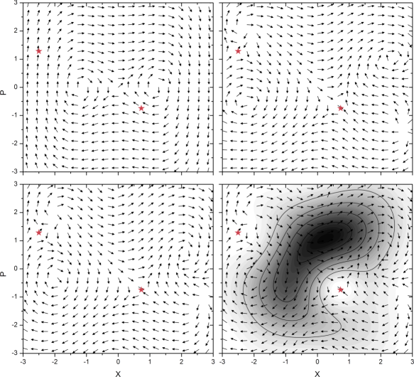
Figure 1: (Color online) Husimi flow at $t=3.5$. The unit arrows indicate the direction of the current, regardless of the intensity. Upper left: $\hbar^{0}$ (classical flow); upper right: $\hbar^{1}$ correction; lower left: $\hbar^{2}$ correction; lower right: $\hbar^{3}$ correction (exact Husimi flow). The red stars mark the zeros of the Husimi function (plotted as background in the last image (white for 0 and dark gray for highest intensity).

Figure 1 shows the direction of the flow at time $t=3.5$ using increasingly accurate approximations. For the hamiltonian (30) the highest $\hbar$ power in the flow series is $q_{max}=3$ and the panels show the classical flow $q=0$, the first order semiclassical correction $q=1$, the next order $q=2$ and the exact result corresponding to $q=3$, for which the Husimi function is also shown as a grey scale contour plot. The corrections in increasing powers of $\hbar$ change the overall structure of the current portraits. The center stationary points present in the classical flow are displaced from their locations both in momentum and position. It can also be seen that additional critical points appear close to the zeros of the Husimi function, and exactly at the zeros they are saddle points of the flow.

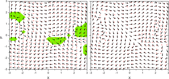
Figure 2: (Color online) Comparison of flow vectors. Thick black arrows are the exact currents and thin red arrows show lower order corrections: $q=0$ on the left and $q=1$ on the right. The shaded green areas in the left panel show regions where momentum inversion occurs.

Figure 2 shows a comparison between the exact and classical flows (left panel) and between the exact and the first order correction (right panel). Except for some small displacements, the $\hbar^{1}$ correction almost mimics the exact quantum flow.

Classically, a particle moves towards the positive position direction if it has a positive momentum and vice-versa. This can be clearly seen in Fig.1(a): if $p>0$ the flow is to the right and if $p<0$ it points to the left. The quantum flow, on the other hand, Fig. 1(d) does not follow that rule everywhere in phase space. There are regions (shaded green areas in Figure 2) where $p>0$ ($p<0$) that have flow lines pointing towards the left (right), the classically wrong direction. This counter-classical motion can be interpreted as an evidence of tunneling represented in this phase space formulation.

Figure 3 shows the zeros and the flow of the Husimi function for the double well potential at different times. The zeros of the Husimi function completely characterize a quantum state leboeuf90 ; cibils92 ; nonnen97 ; korsch97 . For eigenstates the zeros are static (the so called stellar representation), but for general states the zeros usually display a non-trivial dynamics. Absent in the initial state, the zeros approach the region near the wells coming from infinity and move along trajectories that are neither classical nor follows the Husimi flow. We identified that the zeros of the Husimi function correspond to saddle points of the Husimi flow, as seen in Figure 3, and found no other saddle points except those located over the Husimi zeros. We speculate that for every additional zero of the Husimi function there must exist a center of stability in order to conserve the total index of the flow on the phase space (Figure 3).

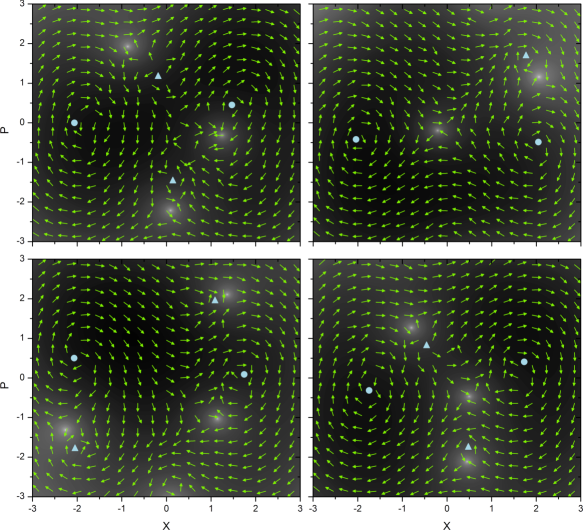
Figure 3: (Color online) Logarithmic plot of the Husimi function superposed with the current unit vectors. White denotes small values ($10^{-10}$) and black the highest ($10^{0}$) for the function. Upper left $t=1.0$, upper right $t=2.0$, lower left $t=3.0$ and lower right $t=4.0$. The zeros are shown by the white spots. Except for one zero, all the others are followed by a flow center (blue triangles). The shifted classical centers are also indicated (blue circles).

V Final remarks

In this work we constructed the phase space flow for the Husimi representation of a one-particle quantum state. The formulas were tested for a particle in a double well potential. We showed that the flow lines differ substantially from its corresponding classical structure, displacing the stagnation points and modifying their quantity. We also observed momentum reversion of the currents in some areas of the phase space. These reversions had already been observed for the Wigner flow, although there is a difference regarding their interpretation in each of these formulations. The Wigner reversion was conjectured to be caused by the function’s non-posivity, which is usually related to quantumness skr13 . As the Husimi function is positive definite this explanation does not work here and we claim that momentum reversion is a more robust blueprint of quantumness than the negativity of the representation itself (see also ferrie11 ), since it is observed in both representations.

Contrary to the Wigner flow skr13 , the Husimi flow does not allow for the birth or merging of critical points. This seems to be a consequence of the isolation of the Husimi zeros, since they appear to be always associated to saddle points of the flow. For small propagation times the zeros move from infinity into the region where the Husimi function is significant and remain there without bifurcating. Also, the Husimi zeros are followed by a center stagnation point, which appears due to index conservation of the flow.

References

- (1) R.J. Glauber Phys.Rev. 131 2766 (1963).
- (2) L. Cohen J. Math. Phys. 7 781 (1966)
- (3) M. Hillery, R.F. O’Connel, M.O. Scully and E.P. Wigner Phys.Rep.106 121 (1984).
- (4) J.R. Klauder and B.S. Skagerstam, Coherent States, Applications in Physics and Mathematical Physics, World Scientific, Singapore, 1985.
- (5) A.M. Perelomov, Generalized Coherent States and Their Application, Springer-Verlag, Berlin, 1986.
- (6) E.J. Heller, J. Chem. Phys. 62(4) (1975) 1544.
- (7) M.F. Herman and E.Kluk, Chem. Phys. 91 (1984) 27.
- (8) M.V. Berry, Proc. R. Soc. A 423 219 (1989).
- (9) J. Kurchan, P. Leboeuf, M. Saraceno Phys. Rev. A 40 6800 (1989).
- (10) K.G. Kay, J. Chem. Phys. 100(6) (1994) 4377.
- (11) K.G. Kay, J. Chem. Phys. 100 (1994) 4432.
- (12) A.L. Xavier Jr, M.A.M. de Aguiar Phys. Rev. Lett. 79 3323 (1997).
- (13) A.M. O. de Almeida Phys.Rep. 295 265 (1998).
- (14) M. Baranger, M.A.M. de Aguiar, F. Keck, H.J. Korsch and B. Schellaas - J. Phys. A34 (2001) 7227-7286
- (15) W.H. Miller, J. Phys. Chem. A 105 (2001) 2942.
- (16) E. Pollak, J. Shao, J. Phys. Chem. A 107 7112 (2003).
- (17) A.D. Ribeiro, M.A.M. de Aguiar and M. Baranger, Phys. Rev. E 69 (2004) 066204.
- (18) D.V. Shalashilin, M.S. Child, Chem. Phys. 304 103 (2004).
- (19) D.V. Shalashilin, I. Burghardt, J. Chem. Phys. 129 084104 (2008).
- (20) M.A.M. de Aguiar, S.A. Vitiello and A. Grigolo, Chem. Phys. 370 42 (2010).
- (21) T.F. Viscondi, M.A.M. de Aguiar, J. Math. Phys. 52x 052104 (2011).
- (22) T.F. Viscondi, M.A.M. de Aguiar, J. Chem. Phys. 134 234105 (2011).
- (23) A. Donoso, Y. Zheng, C.C. Martens, J. Chem. Phys. 119 5010 (2003).
- (24) H. Bauke, N.R. Itzhak, (2011), arXiv:1101.2683v1.
- (25) O. Steuernagel, D. Kakofengitis, G. Ritter, Phys. Rev. Lett. 110 030401 (2013).
- (26) R.T. Skodje, H.W. Rohrs, J. VanBuskirk, Phys. Rev. A 40 2894 (1989).
- (27) R. Gilmore, C.M. Bowden, L.M. Narducci, Phys. Rev. A 12 1019 (1975).
- (28) W.-M. Zhang, D.H. Feng, R. Gilmore, Rev. Mod. Phys. 62 867 (1990).
- (29) F. Trimborn, D. Witthaut, H.J. Korsch, Phys. Rev. A 77 043631 (2008).
- (30) A. D. Bandrauk, H. Shen, J. Chem. Phys. 99 1185 (1993).
- (31) P. Leboeuf, A. Voros, J. Phys. A 23 1765 (1990).
- (32) M.B. Cibils, Y. Cuche, P. Leboeuf, W.F. Wreszinski, Phys. Rev. A 46 4560 (1992).
- (33) S. Nonnenmacher, A. Voros, J. Phys. A 30 295 (1997).
- (34) H.J. Korsch, C. Müller, H. Wiescher, J. Phys. A 30 L677 (1997).
- (35) C. Ferrie, Rep. Prog. Phys. 74 116001 (2011).