Mixed-field orientation of a thermal ensemble of linear polar molecules

Abstract

We present a theoretical study of the impact of an electrostatic field combined with nonresonant linearly polarized laser pulses on the rotational dynamics of a thermal ensemble of linear molecules. We solve the time-dependent Schrödinger equation within the rigid rotor approximation for several rotational states. Using the carbonyl sulfide (OCS) molecule as a prototype, the mixed-field orientation of a thermal sample is analyzed in detail for experimentally accessible static field strengths and laser pulses. We demonstrate that for the characteristic field configuration used in current mixed-field orientation experiments, a significant orientation is obtained for rotational temperatures below $0.7$ K or using stronger dc fields.

I Introduction

The mixed-field orientation of polar molecules via the interaction with an electric field and a nonresonant laser field is a widespread technique to produce samples of oriented molecules. This method was proposed by Friedrich and Herschbach friedrich:jcp111 ; friedrich:jpca103 , and is based on the dc-field induced coupling between the nearly degenerate pair of states with opposite parity forming the tunneling doublets in the strong laser field regime. A recent experimental and theoretical study has proven that under ns laser pulses the weak dc field orientation is not, in general, adiabatic, and that a time-dependent description of the mixed-field orientation process is required to explain the experimental results nielsen:prl2012 ; omiste_nonadiabatic_2012 . Thus, depending on the field configuration, the orientation of a rotational state could be significantly smaller than the adiabatic prediction. In addition, not all the states present a right-way orientation, and some of them are antioriented.

In a thermal ensemble of molecules, the combination of these right- and wrong-way oriented states gives rise to a weakly oriented molecular beam sakai:prl_90 ; Buck:IRPC25:583 . An enhancement of the orientation could be achieved by employing either lower rotational temperatures or quantum-state selected molecular beams. By using inhomogeneous electric fields, the amount of populated states is significantly reduced creating a quantum-state selected molecular beam, and achieving with this beam an unprecedented degree of orientation ghafur_impulsive_2009 ; kupper:prl102 ; kupper:jcp131 . Cold molecular beams, with typical temperatures of the order of $1$ K, are created in supersonic expansions of molecules seeded in an inert atomic carrier gas even:8068 . Depending on the rotational constant, the molecules could still be distributed over a large number of rotational states in these thermal ensembles. In the present work, we investigate the mixed-field orientation of a thermal sample of polar molecules as the rotational temperature is varied. Our aim is to find the temperature at which the thermal ensemble shows a similar orientation as the quantum-state selected molecular beam.

Herein, we consider a polar linear molecule exposed to an electric field combined with a nonresonant laser pulse, and provide a detailed theoretical analysis of the mixed-field orientation of a thermal sample of this molecule. To do so, we solve the time-dependent Schrödinger equation within the rigid rotor approximation for a large set of rotational states. Taking as prototype example the OCS molecule, we explore the mixed-field orientation as a function of the rotational temperature of the thermal sample for several experimental field configurations. We show that to achieve a significant orientation, rotational temperatures around $0.6$ K and $1$ K are required if either a weak or strong dc fields are applied, respectively. We also present the orientation of individual states and, for some of them, analyze the projections of the time-dependent wave functions on the corresponding adiabatic basis.

The paper is organized as follows: In Sec. II we describe the Hamiltonian of the system and the orientation of a molecular thermal ensemble. The mixed-field orientation of the thermal ensemble as a function of the rotational temperature is analyzed in Sec. III. The conclusions are given in Sec. IV.

II The Hamiltonian and the orientation of a thermal ensemble

We consider a polar linear molecule exposed to a homogeneous static electric field and a nonresonant linearly polarized laser pulse. In the framework of the rigid rotor approximation, the Hamiltonian of this system reads

$$H(t)=H_{r}+H_{\textup{s}}(t)+H_{\textup{L}}(t),$$ ((1))

where $H_{r}$ is the field-free Hamiltonian

$$H_{r}=B\mathbf{J}^{2},$$ ((2))

with $\mathbf{J}$ being the total angular momentum operator and $B$ the rotational constant. The interactions with the electric and laser fields are $H_{\textup{s}}(t)$ and $H_{\textup{L}}(t)$, respectively.

The dc field $\mathbf{E}_{\textup{s}}(t)$ forms an angle $\beta$ with the $Z$-axis and is contained in the $XZ$-plane of the laboratory fixed frame (LFF) $(X,Y,Z)$. The dipole coupling with this field reads

$$H_{\textup{s}}(t)=-\bm{\mu}\cdot\mathbf{E}_{\textup{s}}(t)=-\mu\text{E}_{\textup{s}}(t)\cos\theta_{\textup{s}}$$ ((3))

with $\mathbf{E}_{\textup{s}}(t)=\text{E}_{\textup{s}}(t)(\sin\beta\hat{X}+\cos\beta\hat{Z})$, and $\text{E}_{\textup{s}}(t)$ being the electric field strength. The angle between the dipole moment $\bm{\mu}$ and $\mathbf{E}_{\textup{s}}(t)$ is $\theta_{\textup{s}}$, and $\cos\theta_{\textup{s}}=\cos\beta\cos\theta+\sin\beta\sin\theta\cos\phi$. The angles $\Omega=(\theta,\phi)$ are the Euler angles, which relate the laboratory and molecular fixed frames. The molecule fixed frame (MFF) $(X_{M},Y_{M},Z_{M})$ is defined so that the molecular permanent dipole moment $\bm{\mu}$ is parallel to the $Z_{M}$-axis. Based on the mixed-field orientation experiments kupper:prl102 ; kupper:jcp131 ; nielsen:prl2012 , the dc field is switched on first increasing its strength linearly with time. We ensure that this turning-on process is adiabatic, and once the maximum strength $\text{E}_{\textup{s}}$ is achieved, it is kept constant.

The polarization of the nonresonant laser field is taken parallel to the $Z$-axis. Thus, the interaction of the nonresonant laser field with the molecule can be written as seideman2006

$$H_{\textup{L}}(t)=-\cfrac{\textup{I}(t)}{2c\epsilon_{0}}\Delta\alpha\cos^{2}\theta,$$ ((4))

where $\Delta\alpha$ is the polarizability anisotropy, $\textup{I}(t)$ is the intensity of the laser, $c$ is the speed of light and $\epsilon_{0}$ is the dielectric constant. Note that in Eq. (4) the term $-\alpha_{\perp}\textup{I}(t)/2c\epsilon_{0}$ has been neglected because it represents only a shift in the energy. The laser is a Gaussian pulse with intensity $\textup{I}(t)=\textup{I}_{0}\exp\left(-t^{2}/2\sigma^{2}\right)$, $\textup{I}_{0}$ is the peak intensity, and $\sigma$ is related with the full width half maximum (FWHM) $\tau=2\sqrt{2\ln 2}\sigma$. When the nonresonant laser field is turned on the interaction due to this field is much weaker than the coupling with the dc field.

The time-dependent Schrödinger equation associated to the Hamiltonian ((1)) is solved by means of a second-order split-operator technique feit:jcp82 , combined with the discrete-variable and finite-basis representation methods for the angular coordinates bacic:arpc89 ; corey:jcp92 ; offer:10416 ; sanchezmoreno:PRA.2007 . The basis is formed by the spherical harmonics $Y_{JM}(\Omega)$, which are the eigenstates of the field-free Hamiltonian ((2)). $J$ and $M$ are the rotational and magnetic quantum numbers, respectively. At time $t$, the time-dependent states will be labelled as $\left|J,M,l\right>^{\beta}$_t with $l=e$ and $o$ indicating even or odd parity with respect to the $XZ$-plane, respectively. The labels $J$, $M$ and $l$ refer to the field-free quantum numbers to which they are adiabatically connected and they depend on the way the fields are turned on hartelt_jcp128 .

We consider a thermal sample of molecules and investigate its mixed-field orientation at $t=0$ once the peak intensity $\textup{I}_{0}$ has been achieved. For a rotational temperature $T$, the orientation of a thermal distribution is given by

$$\langle\langle\cos\theta\rangle\rangle_{T}=\sum_{J=0}^{\infty}\sum_{M=-J}^{J}W_{J}^{T}\langle\cos\theta\rangle_{JM}$$

where the orientation of the field-dressed state $\left|J,M,l\right>^{\beta}$₀ is $\langle\cos\theta\rangle_{JMl}={}_{0}$${}^{\beta}\left<J,M,l\right|$$\cos\theta$$\left|J,M,l\right>^{\beta}$₀. The thermal weight of the field-free state $\left|J,M,l\right>$ is

$$W_{J}^{T}=\frac{e^{\frac{-J(J+1)B}{k_{B}T}}}{W^{T}}\qquad W^{T}=\sum_{J=0}^{\infty}(2J+1)e^{\frac{-J(J+1)B}{k_{B}T}}$$ ((5))

with $k_{B}$ being the Boltzman constant.

In many mixed-field orientation experiments, the degree of orientation is measured by the ion imaging method kupper:prl102 ; kupper:jcp131 . The up/down symmetry of the 2D-images of the ionic fragments is experimentally quantified by the ratio $\text{N}_{\text{up}}/\text{N}_{\text{tot}}$, with $\text{N}_{\text{up}}$ being the amount of ions in the upper part of the screen plane, and $\text{N}_{\text{tot}}$ the total number of detected ions. In order to compare with the experimental results nielsen:prl2012 , we also compute the orientation ratio $\text{N}_{\text{up}}/\text{N}_{\text{tot}}$, of this thermal sample on a 2D screen perpendicular to the electric field axis. This is defined as

$$\frac{\text{N}_{\textup{up}}}{\text{N}_{\textup{tot}}}=\sum_{J}\sum_{M=-J}^{J}W_{J}^{T}\frac{\text{N}_{\textup{up}}^{JM}}{\text{N}_{\textup{tot}}^{JM}}$$

where

$$\text{N}_{\textup{up}}^{JM}=\int_{y^{2}+z^{2}\leq 1}\int_{z\geq 0}P_{JM}(y,z)\,dydz,$$ ((6))

and

$$\text{N}_{\textup{tot}}^{JM}=\int_{y^{2}+z^{2}\leq 1}P_{JM}(y,z)\,dydz$$

with $P_{JM}(y,z)$ being the projection on a 2D screen perpendicular to the electric field axis of the probability density associated to the state $\left|J,M,l\right>^{\beta}$₀ omiste:pccp2011 , which includes the alignment selectivity of the probe laser. $y$ and $z$ are the abscissa and ordinate of a 2D coordinate system centered on the screen, due to their relation with the Euler angles $(\theta,\phi)$ their values are restricted to $y^{2}+z^{2}\leq 1$ omiste:pccp2011 .

To rationalize the mixed-field orientation results and illustrate the adiabaticity of this process, the time-dependent wave function is projected on the field-dressed adiabatic states

$$\left|J,M,l\right>^{\beta}_{t}=\sum_{j=0}^{N}\sum_{m_{j}=-j}^{j}C_{jm_{j}l^{\prime}}(t)\left|j,m_{j},l^{\prime}\right>_{\text{p}}^{\beta}$$ ((7))

with $C_{jm_{j}l^{\prime}}(t)={}^{\beta}{}_{\text{p}}\left<j,m_{j},l^{\prime}\right|JMl\rangle^{\beta}_{t}$. This adiabatic basis is formed by the eigenstates $\left|j,m_{j},l\right>_{\text{p}}^{\beta}$ of the adiabatic Hamiltonian, i. e., the Hamiltonian (1) with constant electrostatic field $\text{E}_{\textup{s}}$ and constant laser intensity $\textup{I}=\textup{I}(t)$. For each time $t$, the time-independent Schrödinger equation is solved by expanding the wave function in a basis formed by linear combinations of spherical harmonics that respects the symmetries of the system. Note that for $\left|J,M,l\right>^{\beta}$₀, the closer $|C_{JMl}|^{2}$ to one the more adiabatic is the mixed-field orientation process.

III Results

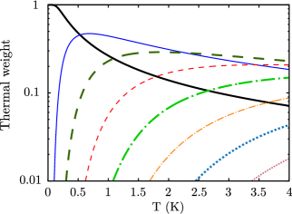
Figure 1: For OCS, thermal weights as a function of the temperature for several $J$-manifolds: $J=0$ (thick solid line), $J=1$ (thin solid line), $J=2$ (thick dashed line), $J=3$ (thin dashed line), $J=4$ (thick dot-dashed line), $J=5$ (thin dot-dashed line), $J=6$ (thick dotted line) and $J=7$ (thin dotted line).

In this work, we use the OCS molecule as prototype. The rotational constant of OCS is $B=0.20286$ cm^-1, the permanent dipole moment $\mu=0.71$ D and the polarizability anisotropy $\Delta\alpha=4.04$ ų. In Fig. 1, we present the thermal weights of several rotational manifolds $(2J+1)W_{J}$, see Eq. (5). Due to the large rotational constant of OCS, the field-free energy splittings are large, and then, the thermal samples with $T\lesssim 1$ K are dominated by the $J=0$ and $J=1$ manifolds. Indeed, the relative weights of the states with $J=0$ and $J=1$ are $W_{0}=47.8\%$ and $W_{1}=44.7\%$ at $T=0.5$ K, and $W_{0}=99.1\%$ and $W_{1}=0.9\%$ at $T=0.1$ K. In our calculations, the thermal sample includes rotational states with $J\leq 9$, and we have ensured that the contribution of higher excitations can be neglected.

We first consider the OCS molecules exposed to an electric field and linearly polarized laser pulse, with both fields parallel to the LFF $Z$-axis. For several field configurations, we present in Fig. 2 the orientation cosine of the thermal ensemble as a function of the temperature for $\text{E}_{\textup{s}}=$300\text{\,}\mathrm{V}\text{/}\mathrm{cm}$$. Note the different scales used in each panel.

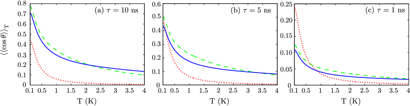
Figure 2: Orientation of a OCS thermal sample $\langle\langle\cos\theta\rangle\rangle_{T}$ as a function of the temperature for Gaussian pulses with $\tau=10$ ns, $\tau=5$ ns, and $\tau=1$ ns and peak intensities $\textup{I}_{0}=${10}^{12}\text{\,}\mathrm{W}\text{/}{\mathrm{cm}}^{2}$$ (thick solid line), $\textup{I}_{0}=$5\text{\times}{10}^{11}\text{\,}\mathrm{W}\text{/}{\mathrm{cm}}^{2}$$ (dashed line) and $\textup{I}_{0}=${10}^{11}\text{\,}\mathrm{W}\text{/}{\mathrm{cm}}^{2}$$ (dotted line). The field configuration is $\text{E}_{\textup{s}}=$300\text{\,}\mathrm{V}\text{/}\mathrm{cm}$$ and $\beta=0^{\circ}$.

For this weak dc field, a significant orientation is only achieved if the rotational temperature is below $0.5$ K, and the Gaussian pulse has $\tau=10$ ns, e. g., for the peak intensities $\textup{I}_{0}=${10}^{12}\text{\,}\mathrm{W}\text{/}{\mathrm{cm}}^{2}$$ and $5\text{\times}{10}^{11}\text{\,}\mathrm{W}\text{/}{\mathrm{cm}}^{2}$ we obtain $\langle\langle\cos\theta\rangle\rangle_{T}\gtrsim 0.5$. Using $1$ ns Gaussian pulse, the orientation of the thermal sample is very small because the rotational states are weakly oriented, for instance, they satisfy $|\langle\cos\theta\rangle_{JMl}|<0.13$ for $\textup{I}_{0}=${10}^{12}\text{\,}\mathrm{W}\text{/}{\mathrm{cm}}^{2}$$ and $\textup{I}_{0}=$5\text{\times}{10}^{11}\text{\,}\mathrm{W}\text{/}{\mathrm{cm}}^{2}$$; whereas for $\textup{I}_{0}=${10}^{11}\text{\,}\mathrm{W}\text{/}{\mathrm{cm}}^{2}$$, we obtain $\langle\cos\theta\rangle_{00e}=0.24$ for the ground state. For these three FWHM, we encounter that a pulse with peak intensity $\textup{I}_{0}=$5\text{\times}{10}^{11}\text{\,}\mathrm{W}\text{/}{\mathrm{cm}}^{2}$$ gives rise to a larger orientation than one with $\textup{I}_{0}=${10}^{12}\text{\,}\mathrm{W}\text{/}{\mathrm{cm}}^{2}$$, this is counterintuitive to what is expected in the adiabatic limit. This phenomenon can be explain by the non-adiabaticity of the mixed-field orientation process nielsen:prl2012 ; omiste_nonadiabatic_2012 , and can be rationalized in terms of the orientation of the individual levels. In Fig. 3, we present the orientation cosine of the field-dressed states $\left|J,|M|,e\right>^{0}$₀ at $t=0$ for two $10$ ns Gaussian pulses with $\textup{I}_{0}=${10}^{12}\text{\,}\mathrm{W}\text{/}{\mathrm{cm}}^{2}$$ and $\textup{I}_{0}=$5\text{\times}{10}^{11}\text{\,}\mathrm{W}\text{/}{\mathrm{cm}}^{2}$$. In these plots, we observe that the levels $\left|J,M,e\right>^{0}$₀–$\left|J+1,M,e\right>^{0}$₀, which form a pendular doublet, are oriented and antioriented, respectively. The $5\text{\times}{10}^{11}\text{\,}\mathrm{W}\text{/}{\mathrm{cm}}^{2}$ pulse is not strong enough to affect the rotational dynamics in the excited rotational states with $J\geq 5$. The pulse with the strongest intensity $\textup{I}_{0}=${10}^{12}\text{\,}\mathrm{W}\text{/}{\mathrm{cm}}^{2}$$ provokes a large orientation on highly excited states with $J\leq 7$. However, for the levels with $J\leq 3$, i. e., those that are important on the cold regime, the $5\text{\times}{10}^{11}\text{\,}\mathrm{W}\text{/}{\mathrm{cm}}^{2}$ pulse gives rise to a larger orientation compared to the ${10}^{12}\text{\,}\mathrm{W}\text{/}{\mathrm{cm}}^{2}$ one. In the parallel field configuration, the population transfer between the two levels forming the doublets in the pendular regime is the only source of nonadiabatic effects in the field-dressed dynamics nielsen:prl2012 ; omiste_nonadiabatic_2012 . For these levels, the population transfer to the neighboring state as the pendular pair is formed is the largest for the strongest laser. For the ground state, at $t=0$ we obtain that the population of the adiabatic state $\left|0,0,e\right>_{\text{p}}^{0}$ is $|C_{00e}|^{2}=0.87$ and $0.91$ with $\textup{I}_{0}=${10}^{12}\text{\,}\mathrm{W}\text{/}{\mathrm{cm}}^{2}$$ and $\textup{I}_{0}=$5\text{\times}{10}^{11}\text{\,}\mathrm{W}\text{/}{\mathrm{cm}}^{2}$$, respectively. As a consequence, the orientation is smallest for $\textup{I}_{0}=${10}^{12}\text{\,}\mathrm{W}\text{/}{\mathrm{cm}}^{2}$$, and, therefore, the thermal ensemble is less oriented. By increasing the temperature, the contribution of excited rotational states becomes important, and the thermal ensemble in a $\textup{I}_{0}=${10}^{12}\text{\,}\mathrm{W}\text{/}{\mathrm{cm}}^{2}$$ pulse shows the largest orientation.

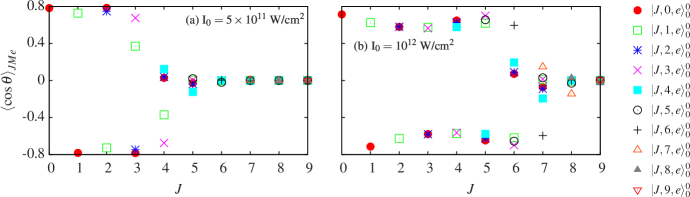
Figure 3: Orientation cosines $\langle\cos\theta\rangle_{JMl}$ at $t=0$ of the states $\left|J,|M|,e\right>^{0}$₀ versus the field-free rotational quantum number $J$. The Gaussian pulses have $\tau=10$ ns, and peak intensities (a) $\textup{I}_{0}=$5\text{\times}{10}^{11}\text{\,}\mathrm{W}\text{/}{\mathrm{cm}}^{2}$$ and (b) $\textup{I}_{0}=${10}^{12}\text{\,}\mathrm{W}\text{/}{\mathrm{cm}}^{2}$$. The field configuration is $\text{E}_{\textup{s}}=$300\text{\,}\mathrm{V}\text{/}\mathrm{cm}$$ and $\beta=0^{\circ}$.

Now, we consider that the electric field is tilted an angle $\beta=30^{\circ}$ with respect to the polarization axis of the laser pulse, that is the LFF $Z$-axis. For several field configurations, we present in Fig. 4 the orientation cosine of the thermal ensemble as a function of the temperature for $\text{E}_{\textup{s}}=$300\text{\,}\mathrm{V}\text{/}\mathrm{cm}$$.

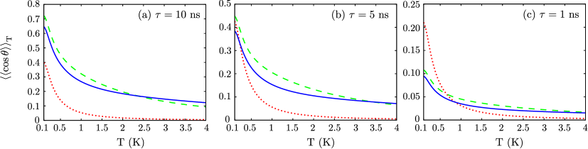
Figure 4: Same as Fig. 2 but for $\beta=30^{\circ}$.

Compared to the parallel field case, the orientation is reduced. For tilted fields, there are two main sources of nonadiabatic effects in the field-dressed dynamics: i) the transfer of population taking place when the quasidegenerate pendular doublets are formed as the laser intensity is increased; ii) at weak laser intensities, there is also population transfer due to the splitting of the states within a $J$-manifold now having the same symmetry. In addition, avoided crossings might be encountered as $I(t)$ is enhanced. The diabatic or adiabatic character of these avoided crossings depends on the field configuration and on the state. Hence, for a certain field configuration, the orientation of the individual states is smaller for $\beta=30^{\circ}$ than for $\beta=0^{\circ}$. This reduction of the orientation is illustrated for the rotational states $\left|J,M,e\right>^{0}$₀ in Fig. 5 for two $10$ ns Gaussian pulses. For $\textup{I}_{0}=$5\text{\times}{10}^{11}\text{\,}\mathrm{W}\text{/}{\mathrm{cm}}^{2}$$, only the states $\left|0,0,e\right>^{0}$₀ and $\left|3,1,e\right>^{0}$₀ present a strong orientation with $|\langle\cos\theta\rangle_{JMl}|>0.6$, whereas for $\textup{I}_{0}=${10}^{12}\text{\,}\mathrm{W}\text{/}{\mathrm{cm}}^{2}$$ only the ground state is strongly oriented. The other levels present a moderate or even small orientation. Due to the population redistribution within a $J$-manifold at weak intensities, the two levels forming a pendular doublet do not possess the same orientation $|\langle\cos\theta\rangle_{JMl}|$ but in opposite directions as occurs in the parallel field configuration.

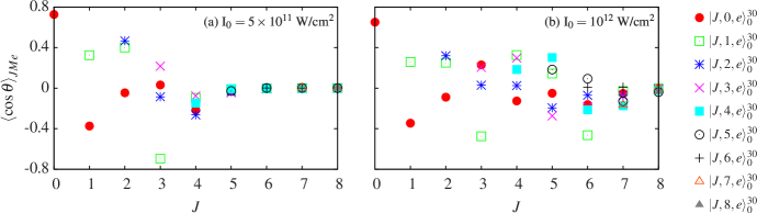
Figure 5: For the states $\left|J,|M|,e\right>^{30}$₀, orientation cosines $\langle\cos\theta\rangle_{JMl}$ at $t=0$ versus the field-free rotational quantum number $J$. The Gaussian pulses have $\tau=10$ ns and peak intensities (a) $\textup{I}_{0}=$5\text{\times}{10}^{11}\text{\,}\mathrm{W}\text{/}{\mathrm{cm}}^{2}$$ and (b) $\textup{I}_{0}=${10}^{12}\text{\,}\mathrm{W}\text{/}{\mathrm{cm}}^{2}$$. The field configuration is $\text{E}_{\textup{s}}=$300\text{\,}\mathrm{V}\text{/}\mathrm{cm}$$ and $\beta=30^{\circ}$.

For the state $\left|2,0,e\right>^{30}$_t, we illustrate its rotational dynamics by presenting the projections of the time-dependent wave function in terms of the adiabatic states in Fig. 6(a) for a $10$ ns pulse with $\textup{I}_{0}=${10}^{12}\text{\,}\mathrm{W}\text{/}{\mathrm{cm}}^{2}$$. The switching on of the electric field has been adiabatic and the level $\left|2,0,e\right>_{\text{p}}^{30}$ is the only one populated when the laser pulse is turned on. At weak laser intensities, the three states with the same symmetry in the $J=2$ manifold, that is $\left|2,0,e\right>_{\text{p}}^{30}$, $\left|2,1,e\right>_{\text{p}}^{30}$ and $\left|2,2,e\right>_{\text{p}}^{30}$, are driven apart: $|C_{20e}(t)|^{2}$ decreases as $\textup{I}(t)$ is increased, whereas $|C_{21e}(t)|^{2}$ and $|C_{22e}(t)|^{2}$ increase. For a wide range of laser intensities, these three coefficients keep their values constant. Around $\textup{I}(t)\approx$2.84\text{\times}{10}^{10}\text{\,}\mathrm{W}\text{/}{\mathrm{cm}}^{2}$$, the states $\left|2,1,e\right>_{\text{p}}^{30}$ and $\left|2,2,e\right>_{\text{p}}^{30}$ suffer an avoided crossings, which is crossed diabatically and the population of these two adiabatic levels is interchanged. Another diabatic avoided crossing is encountered around $\textup{I}(t)\approx$1.09\text{\times}{10}^{11}\text{\,}\mathrm{W}\text{/}{\mathrm{cm}}^{2}$$, and the involved states $\left|2,0,e\right>_{\text{p}}^{30}$ and $\left|3,3,e\right>_{\text{p}}^{30}$ interchanged their population. Upon further increasing $\textup{I}(t)$, the pendular doublets start to form, the coupling between the two involved states increases, and there is a new population redistribution. In this figure, it is appreciated how the different pendular doublets are formed sequentially according to their energy. The first one involves the states $\left|1,0,e\right>_{\text{p}}^{30}$ and $\left|2,2,e\right>_{\text{p}}^{30}$, the next one $\left|2,1,e\right>_{\text{p}}^{30}$ and $\left|2,0,e\right>_{\text{p}}^{30}$, and the third one in this figure $\left|3,3,e\right>_{\text{p}}^{30}$ and $\left|3,2,e\right>_{\text{p}}^{30}$. At $t=0$, the contribution of the adiabatic states to the field-dressed wave function is $|C_{22e}(0)|^{2}=0.11$, $|C_{22e}(0)|^{2}=0.45$, $|C_{21e}(0)|^{2}=0.31$, $|C_{20e}(0)|^{2}=0.08$, $|C_{33e}(0)|^{2}=0.04$ and $|C_{32e}(0)|^{2}=0.01$. As a consequence of this population redistribution, at $t=0$ the state $\left|2,0,e\right>^{30}$₀ is weakly antioriented $\langle\cos\theta\rangle_{20e}=-0.089$, whereas in the adiabatic prediction present a strong anti-orientation $\langle\cos\theta\rangle_{20e}=-0.886$. Analogously, other features of the system such as the energy, alignment, and hybridization of the angular motion are also affected by this population redistribution and do not resemble the adiabatic results.

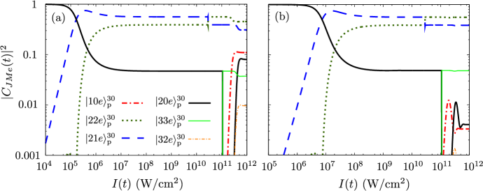
Figure 6: For the state $\left|2,0,e\right>^{30}$_t, we present the squares of the projections of the time dependent wave function onto the adiabatic pendular states versus the laser intensity $\textup{I}(t)$, for dc field strengths (a) $\text{E}_{\textup{s}}=$300\text{\,}\mathrm{V}\text{/}\mathrm{cm}$$ and (b) $\text{E}_{\textup{s}}=$2\text{\,}\mathrm{k}\mathrm{V}\mathrm{/}\mathrm{c}\mathrm{m}$$. The Gaussian pulse has $\tau=10$ ns and peak intensity $\textup{I}_{0}=${10}^{12}\text{\,}\mathrm{W}\text{/}{\mathrm{cm}}^{2}$$, and the fields are tilted an angle $\beta=30^{\circ}$.

For $\beta=30^{\circ}$, the orientation ratio $\text{N}_{\text{up}}/\text{N}_{\text{tot}}$ is presented in Fig. 7. To compute $\text{N}_{\text{up}}/\text{N}_{\text{tot}}$ we have used a probe laser linearly polarized along the vertical axis of the screen detector as in the experiments  nielsen:prl2012 . In these results, we have neglected the volume effect omiste:pccp2011 , we should mention that by including it the value of $\text{N}_{\text{up}}/\text{N}_{\text{tot}}$ will be reduced.

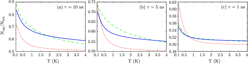
Figure 7: For the OCS thermal sample, we present the orientation ratio $\text{N}_{\text{up}}/\text{N}_{\text{tot}}$ as a function of the temperature for Gaussian pulses with FWHM $\tau=10$ ns, $\tau=5$ ns, and $\tau=1$ ns and peak intensities $\textup{I}_{0}=${10}^{12}\text{\,}\mathrm{W}\text{/}{\mathrm{cm}}^{2}$$ (thick solid line), $\textup{I}_{0}=$5\text{\times}{10}^{11}\text{\,}\mathrm{W}\text{/}{\mathrm{cm}}^{2}$$ (dashed line) and $\textup{I}_{0}=${10}^{11}\text{\,}\mathrm{W}\text{/}{\mathrm{cm}}^{2}$$ (doted line). The field configuration is $\text{E}_{\textup{s}}=$300\text{\,}\mathrm{V}\text{/}\mathrm{cm}$$ and $\beta=30^{\circ}$.

In recent experiments nielsen:prl2012 , for a state selected molecular beam of OCS, $92\%$ in $\left|0,0,e\right>^{0}$₀, $4\%$ in $\left|1,1,e\right>^{0}$₀ and $4\%$ in $\left|1,1,o\right>^{0}$₀, an orientation ratio of $\text{N}_{\text{up}}/\text{N}_{\text{tot}}=0.73$ was achieved using a $8$ ns YAG laser with $\textup{I}_{0}=$9.1\text{\times}{10}^{11}\text{\,}\mathrm{W}\text{/}{\mathrm{cm}}^{2}$$, $\text{E}_{\textup{s}}=$286\text{\,}\mathrm{V}\text{/}\mathrm{cm}$$ and $\beta=30^{\circ}$. Using a $10$ ns pulse, similar results for the orientation ratio of the thermal ensemble are reached if the rotational temperature is sufficiently low. For instance, $\text{N}_{\text{up}}/\text{N}_{\text{tot}}\gtrsim 0.73$ for $T\lesssim 0.65$ K and $0.46$ K with peak intensities $\textup{I}_{0}=$5\text{\times}{10}^{11}\text{\,}\mathrm{W}\text{/}{\mathrm{cm}}^{2}$$ and $\textup{I}_{0}=${10}^{12}\text{\,}\mathrm{W}\text{/}{\mathrm{cm}}^{2}$$, respectively. At $T=0.65$ K, the field-free thermal ensemble is formed by $38.56\%$ OCS in its ground state, $47.19\%$ in $J=1$ and $13\%$ in $J=2$; whereas for $T=0.46$ K, $51.08\%$ have $J=0$, $43.07\%$ $J=1$, and $5.7\%$ $J=2$. For $\tau=5$ ns, only when more than $95\%$ of OCS molecules are in the ground state and $\textup{I}_{0}=$5\text{\times}{10}^{11}\text{\,}\mathrm{W}\text{/}{\mathrm{cm}}^{2}$$ we obtain a similar orientation ratio as in the experiment. By reducing the FWHM to $1$ ns, the orientation ratio is significantly reduced.

An important ingredient to obtain realistic screen images and orientation ratios is the alignment selectivity of the probe laser, which depends on its polarization omiste:pccp2011 . Here, we consider a thermal sample in a laser pulse with $\tau=10$ ns and $\textup{I}_{0}=${10}^{12}\text{\,}\mathrm{W}\text{/}{\mathrm{cm}}^{2}$$, and electric field $\text{E}_{\textup{s}}=$300\text{\,}\mathrm{V}\text{/}\mathrm{cm}$$ and $\beta=30^{\circ}$. In Fig. 8, we present its orientation ratio using the probe pulse with three possible polarizations. For a probe pulse linearly polarized parallel to the vertical axis of the screen, $\text{N}_{\text{up}}/\text{N}_{\text{tot}}$ is the largest because such a pulse favors the Coulomb explosion of the oriented molecules. In contrast, if the probe pulse is linearly polarized perpendicular to screen, the probability of the Coulomb explosion for the oriented molecules is reduced, and, therefore, $\text{N}_{\text{up}}/\text{N}_{\text{tot}}$ presents the smallest values. The circularly polarized probe laser ensures that any molecule is ionized and detected with the same probability independently of the angle $\beta$, and provides the intermediate values of $\text{N}_{\text{up}}/\text{N}_{\text{tot}}$ for any temperature. For a given state, there is no analytical relation between its orientation $\langle\langle\cos\theta\rangle\rangle_{T}$ and the orientation ratio $\text{N}_{\text{up}}/\text{N}_{\text{tot}}$ of the 2D projection of its wave function, although the approximation $\text{N}_{\text{up}}/\text{N}_{\text{tot}}\approx(1+\langle\langle\cos\theta\rangle\rangle_{T})/2$ could be used to obtain an estimation. For instance, a $0.29$ K thermal sample presents an orientation of $\langle\langle\cos\theta\rangle\rangle_{T}=0.506$, and orientation ratios $\text{N}_{\text{up}}/\text{N}_{\text{tot}}=0.757$ and $0.774$ for a probe laser linearly polarized perpendicular and parallel to the screen detector, respectively, and $\text{N}_{\text{up}}/\text{N}_{\text{tot}}=0.761$ for a circularly polarized one. These results should be compared with the value $0.753$ given by this approximation, which provides a lower bound for these three polarizations.

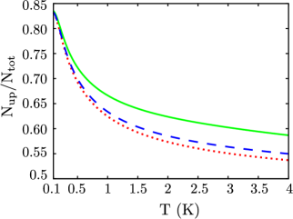
Figure 8: For a OCS thermal sample, we present the orientation ratio $\text{N}_{\text{up}}/\text{N}_{\text{tot}}$ using a probe pulse linearly polarized along the vertical axis of the screen (thick solid line), along the perpendicular axis to the screen (dashed line) and circularly polarized in a plane perpendicular to the screen (doted line). The field parameters are $\tau=10$ ns, $\textup{I}_{0}=${10}^{12}\text{\,}\mathrm{W}\text{/}{\mathrm{cm}}^{2}$$, $\text{E}_{\textup{s}}=$300\text{\,}\mathrm{V}\text{/}\mathrm{cm}$$ and $\beta=30^{\circ}$.

For parallel fields, if the electric field strength is increased, the energy splitting in a pendular doublet is increased, and as a consequence, the degree of adiabaticity in the molecular mixed-field orientation is also enhanced. However, this statement only holds for the ground state of the two irreducible representations if the fields are tilted. For an excited rotational state, a strong dc field does not ensure a large orientation because the coupling between levels with different field-free $M$ values becomes important, and this affects the molecular dynamics. In contrast, for a weak dc field, the mixing between these states is so small that $M$ can be considered as conserved.

In Fig. 9, we plot $\langle\langle\cos\theta\rangle\rangle_{T}$ and $\text{N}_{\text{up}}/\text{N}_{\text{tot}}$ for a thermal sample exposed to a $10$ ns pulse combined with a dc field of $\text{E}_{\textup{s}}=$2\text{\,}\mathrm{k}\mathrm{V}\mathrm{/}\mathrm{c}\mathrm{m}$$ tilted an angle $\beta=30^{\circ}$. For cold samples with $T\lesssim 0.74$ K and $T\lesssim 0.69$ K, we obtain $\langle\langle\cos\theta\rangle\rangle_{T}\gtrsim 0.5$ with $\textup{I}_{0}=${10}^{12}\text{\,}\mathrm{W}\text{/}{\mathrm{cm}}^{2}$$ and $5\text{\times}{10}^{11}\text{\,}\mathrm{W}\text{/}{\mathrm{cm}}^{2}$, respectively. For $\textup{I}_{0}=$5\text{\times}{10}^{11}\text{\,}\mathrm{W}\text{/}{\mathrm{cm}}^{2}$$ and ${10}^{12}\text{\,}\mathrm{W}\text{/}{\mathrm{cm}}^{2}$, we obtain $\text{N}_{\text{up}}/\text{N}_{\text{tot}}\gtrsim 0.73$ if the rotational temperature is $T\lesssim 1.1$ K. Thus, using this strong dc field the orientation of a thermal ensemble becomes comparable to the experimental value for a quantum-state selected molecular beam in a very weak electric field. For this strong electric field, the orientation of the quantum-state selected beam is $\text{N}_{\text{up}}/\text{N}_{\text{tot}}=0.99$ using a probe pulse linearly polarized along the vertical axis of the detector.

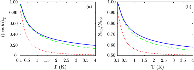
Figure 9: For a OCS thermal sample, we present (a) $\langle\langle\cos\theta\rangle\rangle_{T}$ and (b) $\text{N}_{\text{up}}/\text{N}_{\text{tot}}$ as a function of the temperature for a $10$ ns Gaussian pulse with peak intensities $\textup{I}_{0}=${10}^{12}\text{\,}\mathrm{W}\text{/}{\mathrm{cm}}^{2}$$ (thick solid line), $\textup{I}_{0}=$5\text{\times}{10}^{11}\text{\,}\mathrm{W}\text{/}{\mathrm{cm}}^{2}$$ (dashed line) and $\textup{I}_{0}=${10}^{11}\text{\,}\mathrm{W}\text{/}{\mathrm{cm}}^{2}$$(doted line). The field configuration is $\text{E}_{\textup{s}}=$2\text{\,}\mathrm{k}\mathrm{V}\mathrm{/}\mathrm{c}\mathrm{m}$$ and $\beta=30^{\circ}$.

In Fig. 10, we present the expectation value $\langle\cos\theta\rangle_{JMl}$ at $t=0$ for several rotational states in $10$ ns Gaussian pulses with $\textup{I}_{0}=$5\text{\times}{10}^{11}\text{\,}\mathrm{W}\text{/}{\mathrm{cm}}^{2}$$ and ${10}^{12}\text{\,}\mathrm{W}\text{/}{\mathrm{cm}}^{2}$, $\text{E}_{\textup{s}}=$2\text{\,}\mathrm{k}\mathrm{V}\mathrm{/}\mathrm{c}\mathrm{m}$$ and $\beta=30^{\circ}$. For both field configurations, the $\left|0,0,e\right>^{30}_{0}$ and $\left|3,1,e\right>^{30}_{0}$ states are strongly oriented and antioriented, respectively.

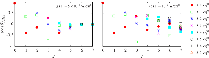
Figure 10: For the states $\left|J,M,e\right>^{30}$₀, we present the orientation cosines $\langle\cos\theta\rangle_{JMl}$ at $t=0$ versus the field-free rotational quantum number. The FWHM of the Gaussian pulses is $\tau=10$ ns and the peak intensities (a) $\textup{I}_{0}=$5\text{\times}{10}^{11}\text{\,}\mathrm{W}\text{/}{\mathrm{cm}}^{2}$$ and (b) $\textup{I}_{0}=${10}^{12}\text{\,}\mathrm{W}\text{/}{\mathrm{cm}}^{2}$$. The field configuration is $\text{E}_{\textup{s}}=$2\text{\,}\mathrm{k}\mathrm{V}\mathrm{/}\mathrm{c}\mathrm{m}$$ and $\beta=30^{\circ}$.

The remaining states show a moderate or weak orientation. The effect of doubling the peak intensity is not noticeable for the levels with field-free rotational quantum number $J\leq 3$, and, in addition, for a certain peak intensity, we encounter similar orientation using a Gaussian pulse of $10$ ns or $5$ ns. The rotational dynamics of the ground state is adiabatic for both pulses; whereas for the excited state, this phenomenon can be explained by the non adiabatic effects taking place at weak laser intensities. When the levels in a certain $J$ manifold are driven apart by the laser field, the process is nonadiabatic and there is a population transfer between them, already at weak laser intensities. Thus, the wave function of any excited level has contributions from adiabatic states which correspond to different pendular doublets. By further increasing the laser intensity, the molecular dynamics is affected by the avoided crossings with adjacent levels having different field-free magnetic quantum numbers $M$ and by the formation of these pendular doublets. The rotational dynamics in most of these crossings will be nonadiabatic and has to be analyzed for each specific state. When the electric field is strong, the energy splitting within the states in the pendular pair is sufficiently large, and, as a consequence, the population transfer when the doublets are formed is not significant.

For completeness, in Fig. 6(b) we present the field-dressed rotational dynamics of the state $\left|2,0,e\right>^{30}$_t in a $10$ ns pulse with $\textup{I}_{0}=${10}^{12}\text{\,}\mathrm{W}\text{/}{\mathrm{cm}}^{2}$$ and a strong dc field of $\text{E}_{\textup{s}}=$2\text{\,}\mathrm{k}\mathrm{V}\mathrm{/}\mathrm{c}\mathrm{m}$$. After an adiabatic switching on of the electric field, the states in the $J=2$ manifold are driven apart, $|C_{20e}(t)|^{2}$ decreases as $\textup{I}(t)$ is increased, whereas $|C_{21e}(t)|^{2}$ and $|C_{22e}(t)|^{2}$ increase. Compared to the weak dc field case in Fig. 6(a), this $J$-manifold splitting takes place at a stronger laser intensity, because the energy gap between the adiabatic states $\left|2,2,e\right>_{\text{p}}^{30}$, $\left|2,1,e\right>_{\text{p}}^{30}$ and $\left|2,0,e\right>_{\text{p}}^{30}$ is larger for $\text{E}_{\textup{s}}=$2\text{\,}\mathrm{k}\mathrm{V}\mathrm{/}\mathrm{c}\mathrm{m}$$ than for $\text{E}_{\textup{s}}=$300\text{\,}\mathrm{V}\text{/}\mathrm{cm}$$. Let us mention that by further increasing $\text{E}_{\textup{s}}$, the energy splitting within this $J$-manifold is increased, and, therefore, this population redistribution will be reduced omiste_nonadiabatic_2012 . The avoided crossing between the states $\left|2,1,e\right>_{\text{p}}^{30}$ and $\left|2,2,e\right>_{\text{p}}^{30}$ occurs at $\textup{I}(t)\approx$2.96\text{\times}{10}^{10}\text{\,}\mathrm{W}\text{/}{\mathrm{cm}}^{2}$$, whereas the one involving the levels $\left|2,0,e\right>_{\text{p}}^{30}$ and $\left|3,3,e\right>_{\text{p}}^{30}$ around $\textup{I}(t)\approx$1.09\text{\times}{10}^{11}\text{\,}\mathrm{W}\text{/}{\mathrm{cm}}^{2}$$. Again, both of them are crossed diabatically, and the population of the adiabatic states is interchanged. By further increasing $\textup{I}(t)$, the pendular doublets start to form. In this case, the dc field is stronger and the energy gap is larger but the coupling due to the ac field is the same, then the population transfer is reduced. Indeed, the adiabatic states $\left|1,0,e\right>_{\text{p}}^{30}$, $\left|2,0,e\right>_{\text{p}}^{30}$ and $\left|3,2,e\right>_{\text{p}}^{30}$, the partners in the pendular doublets of $\left|2,2,e\right>_{\text{p}}^{30}$, $\left|2,1,e\right>_{\text{p}}^{30}$ and $\left|3,3,e\right>_{\text{p}}^{30}$, respectively, show a small population, which is below $0.01$ once the peak intensity at $t=0$ is achieved. Thus, the population at $t=0$ for the field-dressed state $\left|2,0,e\right>^{30}_{0}$ is $|C_{22e}(0)|^{2}=0.56$, $|C_{21e}(0)|^{2}=0.39$, and $|C_{33e}(0)|^{2}=0.05$. These results are similar for the four pulses formed by combining $\tau=5$ ns and $10$ ns with $\textup{I}_{0}=$5\text{\times}{10}^{11}\text{\,}\mathrm{W}\text{/}{\mathrm{cm}}^{2}$$ and ${10}^{12}\text{\,}\mathrm{W}\text{/}{\mathrm{cm}}^{2}$.

IV Conclusions

In this work, we investigate the mixed-field orientation dynamics of a thermal sample of linear molecules. We solve the time-dependent Schrödinger equation within the rigid rotor approximation for a large set of rotational states. As prototype example, we use the OCS molecule. However, we stress that the above results could be used to describe the mixed-field orientation of a thermal ensemble of other polar linear molecules by rescaling the Hamiltonian ((1)) in terms of the rotational constant.

By considering prototypical field configurations with weak dc fields, as in current mixed-field orientation experiments, we have proven that the rotational temperature of the molecular beam should be smaller than $0.7$ K to achieve a significant orientation. Using a weak electric field, if the aim is a strongly oriented molecular ensemble, this should be as pure as possible in the ground state. Thus, it is required a quantum-state-selected molecular beam, unless the rotational temperature could be efficiently reduced below $1$ K. It is found that a significant orientation is achieved for $1$ K molecular samples when the electric field strength is increased.

References

References

- (1) Friedrich B and Herschbach D R 1999 J. Chem. Phys. 111 6157
- (2) Friedrich B and Herschbach D 1999 J. Phys. Chem. A 103 10280
- (3) Nielsen J H, Stapelfeldt H, Küpper J, Friedrich B, Omiste J J and González-Férez R 2012 Phys. Rev. Lett. 108 193001
- (4) Omiste J J and González-Férez R 2012 Phys. Rev. A 86 043437
- (5) Sakai H, Minemoto S, Nanjo H, Tanji H and Suzuki T 2003 Phys. Rev. Lett. 90 083001
- (6) Buck U and Fárník M 2006 Int. Rev. Phys. Chem. 25 583
- (7) Ghafur O, Rouzee A, Gijsbertsen A, Siu W K, Stolte S and Vrakking M J J 2009 Nat Phys 5 289–293
- (8) Holmegaard L, Nielsen J H, Nevo I, Stapelfeldt H, Filsinger F, Küpper J and Meijer G 2009 Phys. Rev. Lett. 102 023001
- (9) Filsinger F, Küpper J, Meijer G, Holmegaard L, Nielsen J H, Nevo I, Hansen J L and Stapelfeldt H 2009 J. Chem. Phys. 131 064309
- (10) Even U, Jortner J, Noy D, Lavie N and Cossart-Magos C 2000 J. Chem. Phys. 112 8068
- (11) Seideman T and Hamilton E 2006 Adv. Atom. Mol. Opt. Phys. 52 289
- (12) Feit M D, Fleck Jr J A and Steiger A 1982 J. Comp. Phys. 47 412
- (13) Bac̆ic̀ Z and Light J C 1989 Annu. Rev. Phys. Chem. 40 469
- (14) Corey G C and Lemoine D 1992 J. Chem. Phys. 97 4115
- (15) Offer A R and Balint-Kurti G G 1994 J. Chem. Phys. 101 10416–10428
- (16) Sánchez-Moreno P, González-Férez R and Schmelcher P 2007 Phys. Rev. A 76 053413
- (17) Härtelt M and Friedrich B 2008 J. Chem. Phys. 128 224313
- (18) Omiste J J, Gärttner M, Schmelcher P, González-Férez R, Holmegaard L, Nielsen J H, Stapelfeldt H and Küpper J 2011 Phys. Chem. Chem. Phys. 13 18815–18824