On the nature of the phase transitions in two-dimensional type II superconductors

Abstract

We have simulated the thermodynamics of vortices in a thin film of a type-II superconductor. We make the lowest Landau level approximation, and use quasi-periodic boundary conditions. Our work is consistent with the results of previous simulations where evidence was found for an apparent first order transition between the vortex liquid state and the vortex crystal state. We show, however, that these results are just an artifact of studying systems which are too small. There are substantial difficulties in simulating larger systems using traditional approaches. By means of the optimal energy diffusion algorithm we have been able to study systems containing up to about one thousand vortices, and for these larger systems the evidence for a first order transition disappears. By studying both crystalline and hexatic order, we show that the KTHNY scenario seems to apply, where melting from the crystal is first to the hexatic liquid state and next to the normal vortex liquid, in both cases via a continuous transition.

I Introduction

It was AbrikosovAbrikosov (1957) who first studied the phase transition from the normal fluid of vortices to the vortex crystal. In a layer of superconducting film of thickness $d$ such that than the effective penetration depthPearl (1964), $(2\lambda^{2}/d)$, is greater than the linear extent $L_{x}$ or $L_{y}$ of the film the Ginzburg-Landau expansion of the free energy can be very accurately approximated as Rosenstein and Li (2010),

$$\frac{F_{\text{GL}}}{k_{B}T^{\text{MF}}_{c}}=d\int d^{2}r\,\left[\alpha(T)|\Psi|^{2}+\frac{\beta_{\kappa}}{2}|\Psi|^{4}+\frac{1}{2m}|\boldsymbol{D}\Psi|^{2}\right],$$ (1)

where $\boldsymbol{D}=-i\hbar\boldsymbol{\nabla}-2e\boldsymbol{A}$, and the vector potential $\boldsymbol{A}$ is that appropriate for a field $B$ normal to the film, $\boldsymbol{A}=(0,Bx,0)$. The temperature-dependent coefficient in this expression, $\alpha(T)$, behaves near the mean-field critical point in zero magnetic field, $T^{\text{MF}}_{c}$, as

$$\alpha(T)=\alpha_{0}\left(T-T^{\text{MF}}_{c}\right).$$ (2)

Abrikosov found the mean-field solution for the functional in Eq. (1) in the LLL (Lowest-Landau-Level) approximation, by minimizing $F_{\text{GL}}$. This yields the solution $\Psi=0$ when $T>T^{\text{MF}}_{c}(B)$ and a solution corresponding to a lattice crystal of vortices when $T<T^{\text{MF}}_{c}(B)$. In his work Abrikosov assumed a crystal with square symmetry, but it was later shown Kleiner et al. (1964) that a triangular lattice has a slightly lower free energy. The transition at the magnetic-field dependent temperature $T^{\text{MF}}_{c}(B)$, which is normally called the $H_{c2}$ line, is a second order transition at mean-field level, and is a transition from a vortex liquid to the vortex crystal phase.

For conventional superconductors the mean-field solution is an excellent first approximation, but fluctuations around the mean-field can never be entirely neglected. The effect of fluctuations on the transition in various dimensions has been studied by renormalization group (RG) methods. An expansion about the upper critical dimension $6$ in $\epsilon$ (when the dimensionality is $6-\epsilon$) was carried out by Brézin, Nelson and Thiaville Brézin et al. (1985) within the LLL approximation. They could not find a stable fixed point and concluded that as a consequence the transition to the crystalline state from the vortex liquid state might be a first order transition. Later measurements of the specific heat of high-temperature superconductors in a field found strong evidence for a first order transitionSchilling et al. (1996) in three dimensional system. However, for the two-dimensional thin film system studied in experiments by Urbach et al.Urbach et al. (1992) there was no sign of a first order transition. On the other hand, a number of Monte Carlo simulations of thin films have indicated that there might be a first order phase transition after all Kato and Nagaosa (1993, 1993); Hu et al. (1994); Šášik and Stroud (1994); Šášik et al. (1995); Li and Nattermann (2003). There have been many other theoretical approaches to vortex lattice melting; these have been extensively reviewed by Rosenstein and LiRosenstein and Li (2010).

In this paper we revisit the problem of simulating two-dimensional superconducting films with quasi-periodic boundary conditions using a novel method Trebst et al. (2004); Bauer et al. (2010). As a consequence we are able to equilibrate larger systems than were studied previously, and have been able to investigate the behavior in more detail by using the microcanonical (constant energy) ensemble. We find that the evidence for a first order transition goes away as the number $N$ of vortices in the simulation is increased. We therefore attribute the apparent evidence for a first order transition in two dimensional superconducting films with quasi-periodic boundary conditions (which geometrically can be thought of as “the flat torus”) to finite size effects.

One of us (MAM) has been arguing for some years that there might be no freezing transition of the vortices in two and three dimensions, and that the correlation length of crystalline short-range order just grew as the temperature $T$ was reduced, reaching infinity only at $T=0$. This argument was partly based on approximate analytical calculations Yeo and Moore (1996, 1996) and general scaling arguments Moore (1997), but also on Monte Carlo simulations where the vortices moved on the surface of a sphere rather than a flat torus Dodgson and Moore (1997); Lee and Moore (1994); O’Neill and Moore (1992). In these simulations on the sphere there was no sign of a first order transition. Since the choice of boundary conditions should not affect thermodynamics in the limit of large $N$, this result is consistent with the finding in this paper that the previously reported first order transition with quasi-periodic boundary conditions is just a finite-size artifact. In the simulations which we are reporting in this paper, the correlation length of crystalline order obtained from the density-density correlation function grows similarly to that reported earlier for the sphere, in that in most of the liquid region, the correlation length seems to be diverging only as $T\to 0$, except that over a narrow temperature interval we find evidence that the hexatic correlation length is diverging to infinity at a finite temperature. This divergence was not observed in the earlier simulations as only the correlation length of crystalline order in the liquid was studied although later some limited evidence was found for a rapidly growing hexatic correlation length Kim and Stephenson .

The divergence at finite temperature of the hexatic correlation length suggests that the KTHNY scenario Halperin and Nelson (1978); Nelson and Halperin (1979); Young (1979) might be relevant. In this scenario the vortex crystal melts at a continuous transition involving the unbinding of dislocations as in the Kosterlitz-Thouless picture Kosterlitz and Thouless (1973) to a hexatic liquid, which in turn changes to a normal liquid at a higher temperature when the disclinations unbind. We believe that this scenario describes our simulations best, although the evidence for the transition from crystal to the hexatic state is not as clear as one might have hoped for, because of finite size effects (see Sec. VI). Recently a cut-down model for the crystal-hexatic transition has been studied Iaconis et al. (2010) which gives results which are also consistent with the KTHNY scenario.

Our interest in this whole topic was reawakened by the investigations of Bowell et al. on the specific heat of niobium Bowell et al. (2010). The niobium studied had a very high degree of purity. No evidence for a first order transition was found. Bossen and SchillingBossen and Schilling (2012) have reviewed the literature on vortex lattice melting of both low and high temperature superconductors and concluded that the first order transition should have been detectable for niobium if the conventional approach to vortex lattice melting applies to it. Our simulations being in two dimensions alas cast no direct light on this mystery. However, in three dimensions the KTHNY theory of the unbinding of topological defects does not apply and a hexatic state is not expected. The apparent absence of a first order transition in very clean niobium could indicate that the old approach of MooreMoore (1997) and the numerical studies in three dimensions Kienappel and Moore (1997) still have utility. The present study in two dimensions appears consistent with the growth predicted in Ref. Moore, 1997 of the correlation length of crystalline order in the vortex liquid phase, that is, it appears to diverge as $T\to 0$, and it only fails to work very close to the temperature at which the topological defects bind. In three dimensions there seems to be no analogue of KTHNY theory and it is possible therefore that the expectations of Ref. Moore, 1997 that there is no true transition in three dimensions remains valid. But we shall leave such speculations to be settled by future work and just concentrate for now on the case of two dimensions.

The three important approximations applied in this paper and commonly used in the large literature on the subject are: the description of a thin film as just a two-dimensional system, the restriction to the Lowest-Landau level and the assumption of a uniform $B$ field. An early paper discussing the first approximation in a theoretical framework is that of Ruggieri and Thouless Ruggeri and Thouless (1976), who argued that if the correlation length in the perpendicular direction, $\xi_{z}$, is larger than the layer thickness $d$, we get a dimensional reduction from three to two. Since this length is divergent at the zero-magnetic field critical temperature, there is always a regime where this approximation applies. The lowest-Landau level approximation has been discussed in detail in the work of Rosenstein and Li Rosenstein and Li (2010). Finally, the success of the analysis of the experimental data in papers such as that by Urbach et al. Urbach et al. (1992), where it is shown that experimental data at different magnetic fields $B$ and temperatures $T$ collapse onto a single curve as a function of the parameter $\alpha_{B}(T)$, (as in our Eq. (26)), shows that all three approximations are applicable to their arrangement of thin films. They used many stacked thin layers with a large separation between them. This means that the magnetic field $B$ is likely to be fairly uniform across the system, so that edge effects, such as fringing fields, can be ignored to a good approximation.

The plan of the paper is as follows. In Sec. II we set up the basis we use to simulate the superconducting film with quasi-periodic boundary conditions. This work is described in some detail (see also Appendix A) because we found it hard to obtain a consistent set of the detailed results needed for doing the simulations from the old literature. In Sec. III we explain how one can extract from the chosen basis set the actual positions of the vortices. This is necessary when we have to calculate the hexatic order parameter and its correlations. It is also needed to construct the Delaunay diagrams showing the topological defects present in the system at various temperatures. In the same section we also discuss the translational symmetry which quasi-periodic boundary conditions allows. We have noticed that for some values of $\sqrt{N}$ there are several distinct orientations possible for the lattice which have exactly the same ground state energy. This feature is studied as it plays a role in the form of the density-density correlation at non-zero temperatures. In Sec. IV and Appendix B we define the correlation functions which we study in the simulation: they include a modified form of the density-density correlation function and also the hexatic correlation function. We also give details of the formalism used to calculate the shear modulus of the system. In Sec. V and Appendices C and D are given details of the Monte Carlo methods which were used and why we found it necessary to use the optimal diffusion algorithm when studying large numbers of vortices. Results are finally discussed in Sec. VI, which is the heart of the paper. We conclude with a discussion of some of the key results in Sec. VII.

II Expansion in a basis

In this paper we choose to model the infinite system by applying quasi-periodic boundary conditions, i.e., by working on the flat torus. Here we shall follow the convention of Yoshioka et al. Yoshioka et al. (1983) and work on a domain of size $[0,L_{x}]\otimes[0,L_{y}]$ with quasi-periodic boundary conditions. Functions satisfying such quasi-periodic boundary conditions have also been considered in mathematics in the theory of $\theta$ functions, and this particular area of research goes by the name “theta-representation of the Heisenberg group” (see the book by Mumford Mumford et al. (2006)); indeed we shall see many of the results rely heavily on the properties of $\theta$ functions.

The most general quasi-periodic boundary conditions are of the form

$$\Psi(x+L_{x},y) =e^{i\theta_{x}}e^{i2\pi Ny/L_{y}}\Psi(x,y),$$ (3)

$$\Psi(x,y+L_{y}) =e^{i\theta_{y}}\Psi(x,y),$$ (4)

where $N$ is an integer, so that

$$\Psi(x+L_{x},y+L_{y})=e^{i(\theta_{x}+\theta_{y})}\Psi(x,y).$$ (5)

We can give a physical interpretation of the boundary conditions in terms of the quantization of the magnetic flux. Since the area for each flux quantum can be expressed in terms of the magnetic length $l_{B}$ as

$$2\pi l_{B}^{2} =h/(2eB),$$ (6)

the periodicity of the wave function requires that

$$L_{x}L_{y} =N2\pi l_{B}^{2}.$$ (7)

The integer $N$ thus specifies the number of vortices on the torus. With the specific choice of quasi-periodic boundary conditions made here, the center of mass of the exactly $N$ zeroes $z^{(0)}_{i}$ of $\Psi$ on the torus, which should be interpreted as the positions of the core of the vortices, is quantized to be Mumford et al. (2006); Haldane and Rezayi (1985)

$$\sum_{i=1}^{N}z^{(0)}_{i}=\left[(n_{x})N_{y}+\frac{\theta_{y}}{2\pi}\right]L_{x}+i\left[(n_{y})N_{x}+\frac{\theta_{x}}{2\pi}\right]L_{y}.$$ (8)

We expand the order parameter field $\Psi$ in terms of quasi-periodic basis functions,

$$\Psi(x,y)=\sum_{j=1}^{N}c_{j}\phi_{j}(x,y;\theta_{x},\theta_{y}),$$ (9)

with Yoshioka et al. (1983); Chung et al. (1997)

$$\phi_{j}(x,y;\theta_{x},\theta_{y}) =\sum_{s=-\infty}^{\infty}f_{j,s}(x)g_{j,s}(y),$$ (10)

where

$$f_{j,s}(x) =\frac{1}{\sqrt{l_{B}\sqrt{\pi}}}\exp\left(-\left(x-X_{js}\right)^{2}/\left(2l_{B}^{2}\right)\right),$$ (11)

$$g_{j,s}(y) =\frac{1}{\sqrt{L_{y}}}\exp\left(i\left(y+\frac{\theta_{x}}{2\pi N}L_{y}\right)X_{js}/l_{B}^{2}\right),$$ (12)

and

$$X_{js} =L_{x}\left[\left(j-\frac{\theta_{y}}{2\pi}\right)\frac{1}{N}+s\right].$$ (13)

This function can be re-expressed in terms of $\theta_{3}$, the Jacobi theta function, also denoted as $\vartheta$ or $\vartheta_{00}$ Mumford et al. (2006),

$$\phi_{j}(x,y;\theta_{x},\theta_{y}) =i\frac{1}{\sqrt{l_{B}L_{x}N\sqrt{\pi}}}\exp\left[\frac{-x^{2}}{2l_{B}^{2}}\right]\exp\left(\frac{\left(i\frac{\theta_{x}}{2\pi N}L_{y}+z\right)^{2}}{2l_{B}^{2}}\right)\theta_{3}\left(\pi\left[\frac{1}{L_{x}}\left(-z+\Theta\right)+\frac{j}{N}\right]\middle|\tau\right),$$ (14)

where

$$z =x+iy,$$ (15)

$$\Theta =\frac{1}{2\pi N}\left[L_{x}\theta_{y}-iL_{y}\theta_{x}\right],$$ (16)

$$\tau =\frac{i}{N}\frac{L_{y}}{L_{x}}.$$ (17)

These basis functions satisfy the boundary conditions

$$\phi_{j}(x+L_{x},y;\theta_{x},\theta_{y}) =e^{i\left(\theta_{x}+2\pi N\frac{y}{L_{y}}\right)}\phi_{j}(x,y;\theta_{x},\theta_{y}),$$ (18)

$$\phi_{j}(x,y+L_{y};\theta_{x},\theta_{y}) =e^{i\theta_{y}}\phi_{j}(x,y;\theta_{x},\theta_{y}),$$ (19)

provided that the quantization condition Eq. (7) is satisfied. It is most easy to interpret the basis functions $\phi_{j}$ by looking at Eqs. (10,11,12). We see that $f$ describes a Gaussian centered at the point $X_{js}$, and $g$ is a plane wave in $y$, with wave vector directly linked to $X_{js}$. Finally, the parameters $\theta_{x}$ and $\theta_{y}$ describe micro-shifts for the vortex positions by $z^{(0)}_{i}\rightarrow z^{(0)}_{i}+\Theta$.

Since the Hamiltonian, as derived below, can easily be show to be independent of the angles $\boldsymbol{\theta}$, we shall from now on take these angles to equal 0. We shall also work on a rectangle shaped to fit a triangular lattice, where

$$L_{y}=\frac{2\sqrt{\pi}l_{B}N_{y}}{\sqrt[4]{3}},\quad L_{x}=\sqrt[4]{3}\sqrt{\pi}l_{B}N_{x},$$ (20)

and the integers $N_{x}$ and $N_{y}$ multiply to give the number of vortices,

$$N_{x}N_{y}=N.$$ (21)

If we decompose the order parameter field in the basis functions (10)

$$\Psi=\mathcal{N}\sum_{j=0}^{N-1}c_{j}\phi_{j},$$ (22)

where $\mathcal{N}$ is a normalization constant, we find that the quadratic term reduces (using orthonormality of the $\phi$’s) to

$$d\sum_{j=0}^{N-1}|c_{j}|^{2}\left[\alpha_{0}\left(T-T^{\text{MF}}_{c}\right)+\frac{e\hbar B}{m}\right]\mathcal{N}^{2}.$$ (23)

This shows that it is useful to introduce a new coupling constant that depends on the magnetic field.

With the choice

$$\mathcal{N}=\pi l_{B}/\sqrt{\beta_{\kappa}},$$ (24)

we can absorb all of the dimensioned factors in a single dimensionless temperature-dependent coupling constant

$$\alpha_{B}(T)=\sqrt{2\pi d/\beta_{\kappa}}\,l_{B}\left(\alpha_{0}\left(T-T^{\text{MF}}_{c}\right)+\frac{e\hbar B}{m}\right),$$ (25)

where $\beta_{\kappa}$ is the strength of the effective quartic term in the GL functional. With a little work (see appendix A) we can now express the Ginzburg-Landau free energy in terms of the $N$ complex variables $c_{i}$,

$$F_{\text{GL}}(\{c\})/\left(k_{B}T^{\text{MF}}_{c}\right)=\frac{\pi}{2}\left(|\alpha_{B}(T)|^{2}\left(\text{sgn}\left(\alpha_{B}(T)\right)\sum_{n=0}^{N-1}|c_{n}|^{2}+\frac{\pi}{2^{3/2}3^{1/4}N_{y}}\sum_{n_{s}=0}^{2N-1}\left|Q_{n_{s}}\right|^{2}\right)\right),$$ (26)

where

$$Q_{n_{s}}=\sum_{n_{p}=0}^{2N-1}\delta_{n_{s}+n_{p},\text{even}}\left[\sum_{s_{p}=-\infty}^{\infty}e^{-\frac{\pi(n_{p}+2Ns_{p})^{2}}{\sqrt{3}N_{y}^{2}}}\right]c_{\left\lceil(n_{p}+n_{s})/2\right\rceil}c_{\left\lceil(n_{p}-n_{s})/2\right\rceil}$$ (27)

is the periodic analogue of a Gaussian weighted convolution between pairs of coefficients on a circle of circumference $N$.

We have introduced a short-hand notation for the periodic continuation of indices,

$$c_{\left\lceil k\right\rceil}\equiv c_{k~{}\text{mod}N}.$$

In summary, we have found that

$$\frac{F_{\text{GL}}(\{c\})}{kT^{\text{MF}}_{c}\,\alpha_{B}(T)^{2}}=E(\{c\})=E_{2}(\{c\})+E_{4}(\{c\}),$$ (28)

with the temperature independent scaled free energy $E$ split into a quadratic and quartic part,

$$E_{2}(\{c\}) =\frac{\pi}{2}\text{sgn}\left(\alpha_{B}(T)\right)\sum_{n=0}^{N-1}|c_{n}|^{2},$$ (29)

$$E_{4}(\{c\}) =\pi^{2}2^{-5/2}3^{-1/4}N_{y}^{-1}\sum_{n_{s}=0}^{2N-1}\left|Q_{n_{s}}\right|^{2},$$ (30)

where $Q_{n_{s}}$ is given in Eq. (27). The energy expression effectively describes the LLL vortex problem as $N$ complex ($2N$ real) coupled quartic oscillators on a circle of radius $N$, with an intermediate range interaction between the oscillators that acts over a distance $\propto N_{y}\sim\sqrt{N}$ along the circle.

We want to simulate the partition function for this model for $N$ vortices (or flux lines)

$$Z(T)=\int e^{-F_{\text{GL}}(\{c\})/kT^{\text{MF}}_{c}}d\{c\},$$ (31)

which can be written as

$$Z(\alpha_{B}(T))=\int e^{-\alpha_{B}^{2}(T)\left(E_{2}(\{c\})+E_{4}(\{c\})\right)}d\{c\}.$$ (32)

Here we use the notation

$$d\{c\}=\prod_{i=1}^{N}d^{2}c_{i}.$$ (33)

III Vortex positions

The wave function $\Psi$ is only an indirect measure of the vortex nature of the system; the square of its absolute value is the vortex density. As we shall see in the next section, we can evaluate density-density correlations directly from $\Psi$, but other important data on the behavior of the system, such as the hexatic order parameter requires that we know the position of the vortices, which are given by the zeroes of $\Psi$. We thus need to find an efficient way to relate a representation in terms of the order parameter wave function to one in terms of its zeroes, and vice-versa.

III.1 $\theta$ functions

It is known, see e.g. Ref. Mumford et al., 2006, that the number of zeroes in the fundamental domain of any quasi-periodic function satisfying the boundary conditions (3,4) is exactly $N$. It is not a trivial task to find their positions from the decomposition in terms of a sum of Jacobi theta functions $\theta_{3}$, Eqs. (14, 22). If we wish to formulate $\Psi$ in terms of its zeroes, it is better to use an alternative expression of $\Psi$ as the product of periodic functions with a single zero in the fundamental domain, i.e., Jacobi functions of the first kind, $\theta_{1}$.

Following Haldane and RezayiHaldane and Rezayi (1985) we thus write the order parameter wave function as a product of $N$ terms each with a zero at the position $z^{(0)}_{i}$,

$$\psi_{\text{prod}}(x,y) =\exp\left(-x^{2}/2l_{B}^{2}\right)$$

$$\quad\exp(ikz)\prod_{i=1}^{N}\theta_{1}\left(\pi(z-z^{(0)}_{i})/L_{x}\middle|\tau^{\prime}\right)$$

$$\equiv\exp(-x^{2}/2l_{B}^{2})\theta_{\text{prod}}(z|\{z^{(0)}\}),$$ (34)

where

$$\tau^{\prime}=i\frac{L_{y}}{L_{x}}$$ (35)

This leads to restrictions for $k$ and for the center of mass (see Ref. Haldane and Rezayi, 1985) [remember that we have chosen the parameters $\theta_{i}$ in Eq. (14), which correspond to the $\phi_{i}$’s in Ref. Haldane and Rezayi, 1985, equal to zero]

$$k=N(m+1)\pi/L_{x},\quad\frac{1}{N}\sum_{i=1}^{N}z^{(0)}_{i}=\frac{n}{N_{x}}L_{x}+i\frac{m}{N_{y}}L_{y}.$$ (36)

The equivalence between Eqs. (22) and (34), up to a normalization constant, will allow useful transformations to be performed.

III.2 Vortex positions from $c$’s

If we wish to determine the vortex positions give the $c$’s, we need to find the zeroes of the product form (34), given the coefficients in the linear “summation” form. To facilitate this calculation, we write, comparing Eq. (34) with Eq. (14),

$$\psi_{\text{sum}}(x,y) =\sum_{j=0}^{N-1}c_{j}\frac{i}{\sqrt{l_{B}L_{x}N\sqrt{\pi}}}\exp\left[\frac{-x^{2}}{2l_{B}^{2}}\right]$$

$$\quad\exp\left(\frac{z^{2}}{2l_{B}^{2}}\right)\theta_{3}\left(\pi\left[-\frac{1}{L_{x}}z+\frac{j}{N}\right]\middle|\tau\right)$$

$$=\exp(-x^{2}/2l_{B}^{2})\theta_{\text{sum }}(z|\{c\}).$$ (37)

We must now solve the equations

$$\theta_{\text{prod}}(z|\{z^{(0)}\})=\theta_{\text{sum}}(z|\{c\})$$ (38)

for the set $\{z^{(0)}\}$. This is a complex non-linear problem. We approach it by first using a contour-finding technique to determine all closed contours of $|\theta_{\text{sum}}|$ for a chosen value near zero. We then determine the center of gravity of each contour, which is usually already a very good approximation to the position of a zero. The position of each $z^{(0)}_{i}$ is then improved by using a root finding algorithm in the complex variable $z$, which normally converges quickly. The remaining normalization of $\theta_{\text{prod}}$ can be found by fixing the value at any point that does not coincide with a root. The most likely scenario for failure of the method is the occurrence of multiple or very close roots, and making small mistakes in the calculation of a vortex that is close to the boundary, thus misidentifying it as inside or outside the fundamental domain.

III.3 Determining $c$’s from vortex positions

Clearly, given only the vortex positions, we can only determine $\theta_{\text{prod}}$ up to a normalization. A change of normalization in the sum-representation (22) corresponds to a simultaneous scaling of all the $c$’s. In other words, the vortex positions alone define a one-dimensional manifold of fields. That means that we have just found that the linear equations stating that there are vortices at all the $z^{(0)}_{i}$’s, i.e., the set of equations ($1\leq j\leq N$)

$$\theta_{\text{sum}}(z^{(0)}_{j}|\{c\})=0,$$ (39)

must have a one-dimensional family of solutions $\{c\}$. This condition can thus be written as the determinantal condition $\det\left(M\right)=0,$ where the entries in the $N\times N$ matrix $M$ take the simple form

$$M_{ij} =\sum_{s=-\infty}^{s=\infty}\exp\left[-\frac{1}{2}\left[2\pi\left(j+Ns\right)\right]^{2}\frac{L_{x}}{L_{y}N}+2\pi\left(j+Ns\right)z^{(0)}_{i}/L_{y}\right].$$ (40)

The coefficients $c_{j}$ are obviously given, up to the unknown normalization constant, by the eigenvector for eigenvalue $0$ (the singular value) of the matrix $M$.

III.4 Symmetry breaking

Since we are studying a 2D system with an interaction of intermediate range, we expect the Mermin-Wagner theorem to hold, so that no spontaneous breaking of continuous symmetries can exist. In other words, the one-body densities satisfy these symmetries. Unfortunately, the flat torus – periodic boundary conditions – inherently breaks both rotational and translational symmetries, and we thus need to consider what spurious effects this may have.

III.4.1 Translations

Since the center-of-mass coordinate can only take a finite number $N$ of values, see Eq. (36), translational symmetry is broken to a discrete subgroup. The number of ground-states has $N$-fold degeneracy, and we could alternatively have used these as a basis for the calculations. This corresponds to the Eilenberger basis, a well-known alternative to the basis choice employed in this workEilenberger (1967).

III.4.2 Rotations

There is only limited room for restoring rotational symmetry on a torus. Whereas we have designed the shape of the fundamental domain to fit one triangular lattice, there are a few special cases where we can fit an the same equilateral-triangular lattice to a flat torus in a different way. Webber (1997); Giomi and Bowick (2008). However, we can easily find many ways to fit a general triangular lattice to a torus, some of which are very close in energy to the ground state. Enumerating the winding around the torus in the standard way for carbon nanotubes, but now in both $x$ and $y$ directions, we find that we can label such a lattice with two integer vectors $\boldsymbol{m}=(m_{1},m_{2})$ and $\mbox{$\boldsymbol{n}$}=(n_{1},n_{2})$, describing the periodic vectors along the $x$ and $y$ axes in terms of the lattice basis, see Fig. 1.

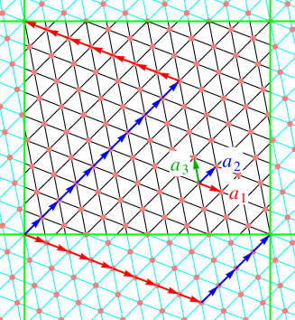
Figure 1: (Color online) A picture of the labeling of a periodic triangular lattice on the flat torus. The fundamental domain is inside the green rectangle, and the lattice connections are shown in black. Each such can be labeled uniquely by two vectors that wrap along the $x$ and $y$-axes, respectively, decomposed in the basis $\boldsymbol{a}_{1}$, $\boldsymbol{a}_{2}$. In the case shown here this label would be $\left(\left(8,4\right),\left(-7,9\right)\right)$.

Since the number of vortices in the fundamental domain is fixed, we find that the vectors satisfy the Diophantine equation

$$m_{1}n_{2}-m_{2}n_{1}=N_{x}N_{y}=N,$$ (41)

where we have added the (simplifying, but not strictly necessary) requirement that the determinant on the left-hand-side is positive. The case of negative determinant can be reached by a simple inversion of one of the the two vectors $\boldsymbol{m}$ or $\boldsymbol{n}$, i.e., a reflection in the $y$ or $x$ axis. There is an issue with the integer labels not being unique; we can choose any two out of the three vectors $\boldsymbol{a}_{i}$ as a basis, and multiply any of these vectors by an overall sign and get a different result for $\boldsymbol{n}$ and $\boldsymbol{m}$, without changing the crystal. The ordering principle we apply is that we always choose the two shortest vectors $\boldsymbol{a}_{i}$, and require that the largest components of each vector $\boldsymbol{a}_{1}$, $\boldsymbol{a}_{2}$ are positive.

An expression for the energy for a crystal of this type can be found in the literature, e.g., Eq. (77) in Ref. Rosenstein and Li, 2010, and can be written as

$$E/N=-\frac{1}{2\beta},$$ (42)

where the parameter $\beta$ is given by the lattice sum

$$\beta=\sum_{k,l=-\infty}^{\infty}\exp\left(-\frac{\pi}{A}\left|k\boldsymbol{a}_{1}+l\boldsymbol{a}_{2}\right|^{2}\right),$$ (43)

and $A$ is the area of the basic triangular unit cell of the crystal. There is an equivalent, but slightly less practical, expression in terms of the elliptic constant $\tau$ Aftalion et al. (2006). The triangular ground state is obtained for the well-known value

$$\beta=\beta_{A}=1.159595,$$ (44)

the “Abrikosov parameter”.

Since we shall always apply this on an $(N_{x},\frac{1}{2}\sqrt{3}N_{y})$ basic lattice (using $\sqrt[4]{3}\sqrt{\pi}l_{B}$ as the unit of length, see Eq. (20)), we find that

$$\left(\begin{array}[]{cc}m_{1}&m_{2}\\ n_{1}&n_{2}\end{array}\right)\left(\begin{array}[]{c}\boldsymbol{a}_{1}\\ \boldsymbol{a}_{2}\end{array}\right)=\left(\begin{array}[]{c}(N_{x},0)\\ (0,N_{y}\sqrt{3}/2)\end{array}\right),$$ (45)

or

$$\left(\begin{array}[]{c}\boldsymbol{a}_{1}\\ \boldsymbol{a}_{2}\end{array}\right) =\frac{1}{N_{x}N_{y}}\left(\begin{array}[]{cc}n_{2}&-m_{2}\\ -n_{1}&m_{1}\end{array}\right)\left(\begin{array}[]{c}(N_{x},0)\\ (0,N_{y}\sqrt{3}/2)\end{array}\right)$$ (52)

$$=\left(\begin{array}[]{c}(n_{2}/N_{y},-m_{2}/N_{x}\sqrt{3}/2)\\ (-n_{1}/N_{y},m_{1}/N_{x}\sqrt{3}/2)\end{array}\right).$$ (55)

The third vector $\boldsymbol{a}_{3}$ is the shortest of

$$((n_{2}\mp n_{1})/N_{y},(-m_{2}\pm m_{1})/N_{x}\sqrt{3}/2).$$ (56)

The lengths squared are thus

$$n_{2}^{2}/N_{y}^{2}+\frac{3}{2}m_{2}^{2}/N_{x}^{2},n_{1}^{2}/N_{y}^{2}+\frac{3}{2}m_{1}^{2}/N_{x}^{2}\\ \text{ and }(n_{1}\pm n_{2})^{2}/N_{y}^{2}+\frac{3}{2}(m_{1}\mp m_{2})^{2}/N_{x}^{2}.$$ (57)

There are two classes of solutions we shall be interested in: First of all states that are close to the crystal aligned with the boundary conditions, and secondly low energy states that are very differently orientated from the default crystal – in the most extreme scenario this will be another ground state with different orientation. In Sec. VI when discussing non-universal behavior we shall analyze the state of almost default orientation, and the solutions to the Diophantine equation (41) for small deformations of the ground state.

IV Correlations

The best way to study the structure of the phase diagram is to look at the correlations that are present. Most of the past Monte Carlo work concentrated on the crystalline correlations; there is some work on the shear modulus, which is linked to the hexatic-crystal phase transition. We shall look at these, but also include hexatic order correlations in our arsenal of analysis tools.

IV.1 Density-density correlations: the function $\Delta$

The most studied correlation function for the vortex problem is a modification of the density-density correlation. We start from

$$g(\boldsymbol{q)} \equiv\int d^{2}r\,d^{2}r^{\prime}e^{i\boldsymbol{q}.(\boldsymbol{r}-\boldsymbol{r}^{\prime})}$$

$$\times\left[\left\langle\left|\Psi(r)\right|^{2}\left|\Psi(r^{\prime})\right|^{2}\right\rangle-\left\langle\left|\Psi(r)\right|^{2}\right\rangle\left\langle\left|\Psi(r^{\prime})\right|^{2}\right\rangle\right]/\mathcal{N}^{4}$$

$$=\left\langle\left|\rho(\boldsymbol{q})\right|^{2}\right\rangle-\left|\left\langle\rho(\boldsymbol{q})\right\rangle\right|^{2},$$ (58)

with

$$\rho(\boldsymbol{q}) =\int d^{2}r|\Psi(r)|^{2}e^{i\boldsymbol{q}\cdot\boldsymbol{r}}/\mathcal{N}^{2}.$$ (59)

We choose

$$q_{y}=k_{y}/l_{B}=m_{y}2\pi/L_{y}=\frac{2\sqrt{\pi}m_{y}}{\sqrt[4]{3}l_{B}N_{y}},$$ (60)

and follow the approach set out in detail in Appendix B.

It is convenient to multiply $g(q)$ by the Gaussian factor $\exp(k^{2}l_{B}^{2}/2)$, to obtain the correlator

$$\Delta(\boldsymbol{k})=\left\langle\left|\delta(\boldsymbol{k})\right|^{2}\right\rangle-\left|\left\langle\delta(\boldsymbol{k)}\right\rangle\right|^{2},$$ (61)

with

$$\delta(\boldsymbol{k})=\sum_{j^{\prime}=0}^{N-1}\left(c_{\left\lceil j^{\prime}\right\rceil}\exp\left(\frac{2i\pi m_{x}j^{\prime}}{N}\right)\right)c_{\left\lceil j^{\prime}+m_{y}\right\rceil}^{*},$$ (62)

This is often normalized to

$$\tilde{\Delta}(\boldsymbol{k})=\Delta(\boldsymbol{k})/\left|\left\langle\delta(0)\right\rangle\right|^{2},$$ (63)

so that the results no longer depend on the normalization of the wave function. The periodicity of the expression (62) shows that both $m_{x}$ and $m_{y}$ take integer values from $0$ to $N-1$. Thus

$$0 \leq k_{x}\leq\frac{\sqrt[4]{3}\sqrt{\pi}\left(N-1\right)}{N_{x}},$$ (64)

$$0 \leq k_{y}\leq\frac{2\sqrt{\pi}(N-1)}{\sqrt[4]{3}N_{y}}.$$ (65)

IV.1.1 Extraction of the correlation length

We would like to use the density-density correlation function to extract a correlation length. The difficulty, as one can see later, e.g., in Fig. 18, is that there is no peak at $k=0$, i.e., there is a correlation hole. The first peaks when we have crystal, or the first ring when we have a liquid, occur at a finite $k$ value. There are various ways to extract a correlation length from these features.

In a liquid, we can take the circular average of the density-density correlation function, and either fit a Lorentzian to the first peak, or look at the curvature of the peak near the top, assuming it is Lorentzian. We find that both of these approaches lead to a very similar value for a correlation length.

In a state where we can see discrete Bragg peaks, the situation is much more complex. Even though the angular average gives the best statistics, it appears to be a less sensible approach. Several of the discrete Bragg peaks correspond to states that are not aligned with the natural crystal axes, and therefore must have some defects or vacancies and some deformation of the remaining crystal structure to fit the simulation box. Thus both the direction and magnitude of the $k$-vector changes. This tends to broaden the apparent peaks, and leads to an underestimate of the correlation length when mixing discrete points at different angles.

Since at least one of the crystalline ground states aligns with the $x$-axis, we instead look at the width near the maximum along this axis in $k$ space, as well as the two lines making an angle $\pi/3$ with this axis. We then determine the correlation length by the curvature at the top of the peak. This measure is sensible both in liquid and crystal-like states, as long as we take account of the fact that the position of the peak in $k$ space varies a little with temperature.

IV.2 Hexatic order parameter

The standard model of 2D melting is the KTHNY scenario, where there is an intermediate phase with hexatic ordering between crystal and liquid. In order to see whether this plays a role, it would be useful to measure the hexatic order parameter $\Psi_{6}$ and its correlation function. If we know the vortex positions, we just need to determine the positions of the nearest neighbors of each vortex, which can be obtained from a Delaunay triangulation, which will give us access to the local coordination number of each vortex of the lattice, as well as a list of $N_{\text{nn}}(\boldsymbol{r}_{i})$ nearest neighbors. We then define an order parameter

$$\Psi_{6}(\boldsymbol{r}_{i})=\frac{1}{N_{\text{nn}}(\boldsymbol{r}_{i})}\sum_{k=1}^{N_{\text{nn}}(\boldsymbol{r}_{i})}\exp(i6\theta_{k}),$$ (66)

where $\theta_{k}$ is the angle between the vector pointing from the vortex at $\boldsymbol{r}_{i}$ to its $k$-th nearest neighbor and the $x$-axis. Notwithstanding the obvious bias in its definition, this quantity is commonly used in the analysis of colloidal systems. We define the hexatic correlation function as

$$\chi_{6}(\boldsymbol{q})=\left\langle\sum_{ij}\Psi_{6}^{*}(\boldsymbol{r}_{i})e^{i\boldsymbol{q}\cdot(\boldsymbol{r}_{j}-\boldsymbol{r}_{i})}\Psi_{6}(\boldsymbol{r}_{j})\right\rangle.$$

A hexatic length parameter is found through the standard Ballesteros-type analysis Ballesteros et al. (2000), and define the correlation length by the width of $\chi_{6}$ as determined by the curvature at the top of the curve,

$$\xi_{6}\equiv\sqrt{(\chi_{6}(0)/\chi_{6}(\boldsymbol{k})-1)}/(2\sin(k/2)).$$ (67)

The only difference with the standard approach, is that we take the average over $\boldsymbol{k}$ as the first allowed reciprocal lattice vector in the $x$ and $y$ directions.

IV.3 Shear Modulus

If we shear the crystal by an angle $\theta$, the shear modulus can be evaluated to be expressed as Šášik and Stroud (1994),

$$\mu =-(k_{B}T/N)\left[\partial_{\theta,\theta}\ln Z(a_{B}(T),\theta)\right]_{\theta=0}$$

$$=\frac{k_{B}T}{N}\biggl{[}\alpha_{B}(T)^{2}\left\langle\partial_{\theta,\theta}E(\{c\},\theta)\right\rangle_{\theta=0}-$$

$$\qquad\alpha_{B}(T)^{4}\left\langle\left(\partial_{\theta}E(\{c\},\theta)\right)^{2}\right\rangle_{\theta=0}\biggr{]}.$$ (68)

We shall refer to $\left\langle\left(\partial_{\theta}E(\{c\},\theta)\right)^{2}\right\rangle_{\theta=0}$ as the shear susceptibility, and $\left\langle\partial_{\theta,\theta}E(\{c\},\theta)\right\rangle_{\theta=0}$ as the shear stiffness, since these labels give a sensible interpretation of these two quantities. We shall see below that it is the shear susceptibility that gives us information about the phases of the system; the shear stiffness is almost temperature independent.

With the choice of boundary conditions as in Eqs. (3,4) the easiest way to implement shearing is in the $y$ direction. As discussed by Šášik et al Šášik and Stroud (1994); Šášik et al. (1995), such a sheared system can be described by the transformation $\Psi(x,y)\rightarrow\Psi(x,y+x\sin\theta)$. The transformation can be absorbed in a change of the basis functions

$$\phi^{\theta}_{j}(x,y) =\phi_{j}(x,y+x\sin\theta)$$

$$=\frac{1}{\sqrt{L_{y}}}\frac{1}{\sqrt{l_{B}\sqrt{\pi}}}\exp\left(-\left(x-X_{js}\right)^{2}/\left(2l_{B}^{2}\right)\right)\exp\left(i\left(y+x\sin\theta\right)X_{js}/l_{B}^{2}\right)$$

$$=\frac{1}{\sqrt{L_{y}}}\frac{1}{\sqrt{l_{B}\sqrt{\pi}}}\exp\left(-\left[{X_{js}}^{2}-{X^{\theta}_{js}}^{2}\right]/\left(2l_{B}^{2}\right)\right)\exp\left(-\left(x-X_{js}^{\theta}\right)^{2}/\left(2l_{B}^{2}\right)\right)\exp\left(iyX_{js}/l_{B}^{2}\right),$$ (69)

where

$$X_{js}^{\theta}=X_{js}(1-i\sin\theta).$$ (70)

If we wrap around the torus in the $x$ direction, we obtain an additional phase in the wave function

$$\phi^{\theta}_{j}(x+L_{x},y) =\sum_{s=-\infty}^{s=\infty}f_{j,s}(x)\exp\left(i\sin\theta L_{x}X_{js}/l_{B}^{2}\right)\frac{1}{\sqrt{L_{y}}}\exp\left(iy\,X_{js}/l_{B}^{2}\right).$$ (71)

It is rather straightforward to obtain the $\theta$ dependence of the scaled free energy

$$E(\{c\},\tan\theta) =\frac{\pi}{2}\sum_{n=0}^{N-1}\left|c_{n}\right|^{2}\text{sgn}\left(\alpha_{B}(T)\right)+\pi^{2}2^{-5/2}3^{-1/4}N_{y}^{-1}\sum_{n_{s}=0}^{2N-1}\left|Q_{n_{s}}(\tan\theta)\right|^{2},$$ (72)

$$Q_{n_{s}}(\tan\theta) =\sum_{n_{p}=0}^{2N-1}\delta_{n_{s}+n_{p},\text{even}}\left[\sum_{s_{p}=-\infty}^{\infty}e^{-\frac{\left(\pi-i\tan(\theta)/2N\right)(n_{p}+Ns_{p})^{2}}{\sqrt{3}N_{y}^{2}}}\right]c_{\left\lceil(n_{p}+n_{s})/2\right\rceil}c_{\left\lceil(n_{p}-n_{s})/2\right\rceil}.$$ (73)

This allows us to calculate the first and second derivatives at $\theta=0$ by

$$\left.\partial_{\tan\theta}E(\{c\},\tan\theta\right|_{\theta=0} =\pi^{2}2^{-5/2}3^{-1/4}N_{y}^{-1}\sum_{n_{s}=0}^{2N-1}(-2)\operatorname{Im}\left(Q_{n_{s}}^{\prime}Q_{n_{s}}^{*}\right),$$

$$\left.\partial_{\tan\theta}^{2}E(\{c\},\tan\theta)\right|_{\theta=0} =\pi^{2}2^{-5/2}3^{-1/4}N_{y}^{-1}\sum_{n_{s}=0}^{2N-1}\left|Q_{n_{s}}^{\prime}\right|^{2}-2\operatorname{Re}\left(Q_{n_{s}}^{\prime\prime}Q_{n_{s}}^{*}\right),$$ (74)

with

$$Q_{n_{s}}^{\prime}=\left[\partial_{\theta}Q_{n_{s}}(\tan\theta)\right]_{\theta=0},\quad Q_{n_{s}}^{\prime\prime}=\left[\partial_{\theta}^{2}Q_{n_{s}}(\tan\theta)\right]_{\theta=0}.\quad$$ (75)

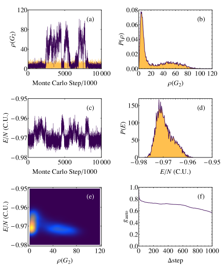
Figure 2: (Color online) An example of a standard Monte Carlo simulation for $\alpha_{B}(T)^{2}=91$, for a system of $16\times 16$ vortices. In (a) we show both a measure of the density-correlation (purple) and average density (yellow) at the point $G_{2}$ – the second smallest $k$ vector in the reciprocal crystal lattice – as a function of the Monte Carlo time. To the right of this (b) we show the probability distribution for the density-density correlation at this point. On the second row we have similar plots for the energy (c) and (d). The final row shows a density plot of $E$ vs. $\rho(G_{2})$ (e), and to the right of this, (f), we show the energy auto-correlation function as a function of the number of Monte Carlo steps.

V Monte Carlo Techniques

As discussed in great detail in Appendix C, C, we have studied the application of three different Monte Carlo techniques: The standard canonical Metropolis algorithm, and two microcanonical ones (sometimes referred to as “broad-histogram techniques”), the Wang-Landau and the optimal energy diffusion algorithm.

The reason we have not persisted with the use of the standard Metropolis sampling of the Boltzmann factor, is that, as shown below, there appear to be serious difficulties with obtaining reproducible results. This points to a long time scale associated with diffusion through the abstract configuration space, especially at certain temperatures. Such behavior is commonly associated with a phase transition.

To really study the detailed behavior in the interesting temperature range, one might use parallel tempered Monte Carlo Neuhaus et al. (2007). In such simulations one often reverts to “reweighting” the results to a single temperature to get the temperature dependent probability distribution $P(E,T)$. We follow a different route that gives us more direct access to the underlying density of state.

As we shall show below, most of the relevant information is actually contained in the microcanonical density of states $g(E)$, and especially the derivative of its logarithm,

$$S_{\text{mc}}(E)=\frac{d}{dE}\ln g(E).$$ (76)

There is a very powerful algorithm that directly determines $g(E)$, the Wang-Landau algorithm Wang and Landau (2001). As discussed in Appendix C, it is very different from a standard Monte Carlo algorithm, since the simulation weights are being updated as the simulation progresses, finally converging to the density of states.

As argued cogently in Ref. Wu et al., 2005, this algorithm can run into difficulties if there are barriers to the Monte Carlo process, modeled as a random walk as a function of energy. In the problem we are considering these barriers appear to be substantial – which is closely linked to the apparent first order nature of the phase transition for smaller system sizes. Also, it is not very simple to write parallel versions of the Wang-Landau algorithm.

The approach from Ref. Trebst et al., 2004, where we optimize the current in the random walk between the extremes in energy, seems to give the best of both worlds. It is microcanonical, and the diffusion becomes optimal as the simulation progresses. As a by-product we obtain an understanding where barriers to energy diffusion are – and there are clear links between the barriers and the associated phase structure.

As will be shown below, the optimal energy diffusion algorithm proved the most illuminating for the problem studied here.

VI Results

In the results reported in this section, we use a unit of energy where the crystalline state for $N$ vortices has a natural value $E=-N$; this means that we scale the energy as defined in Eqs. (28,30) by twice the Abrikosov parameter (44), i.e., we multiply these expressions by $2\beta_{A}$. Expressed in these units, the crystalline state thus has energy $E(\{c_{\text{crystal}}\})/N=-1$. Such units will be denoted as “C.U.” below.

Our first set of simulations uses the classical Metropolis Monte Carlo algorithm without optimizations. We obtain results of similar quality to those which can be found in the literature for lattice sizes of up to about 14 by 14 – we find that around that point results have rather limited reproducibility with a sensible length of simulation. A typical example of a set of simulations just beyond that size is shown in Fig. 2. Here we analyze a system with $256$ vortices (boundary conditions are chosen such that the lowest energy state is a triangular lattice of 16 rows of 16 vortices each). In that figure we show both energy and the density fluctuations at a suitably chosen point of the triangular lattice, for $\alpha_{B}(T)^{2}=91$, which is at a temperature where we see phase-coexistence. We can clearly see the density fluctuations suggestive of a two-phase system; the energy seems to behave similarly, even though the correlation between energy and density on the final row shows a more complicated picture. Nevertheless, it is entirely possible to pick out two populations. Finally the energy auto-correlation of the Monte Carlo process shows fast decay for a few steps, and then little or no decay. We were very concerned when we first saw this behavior, since it seems to invalidate the simulations. A simple statistical model with $P(E)$ the sum of two disjoint Gaussian probability distributions shows exactly this behavior, so it may be that energy autocorrelation is not a very good quality measure in an area of phase coexistence. The density plot of energy versus $\rho(G_{2})$ lends support to such a model.

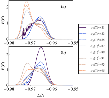
Figure 3: (Color online) The $P(E)$ curves for the $16\times 16$ system, rescaled to a single value of $\alpha_{B}(T)^{2}=90.1$. The curves are normalized to cross at a single point, $E/N=-0.968\ \text{C.U.}$, which is roughly in the middle of the two peaks. Panel (a) shows results for simulations with decreasing $\alpha_{B}(T)^{2}$; panel (b) for increasing values of this parameter.

The fact that we have two distinct populations means that we will find it difficult to simulate reliably near this temperature, as is shown in Fig. 3. There we show results from two groups of simulations. In each series of simulation we use the final configuration from a simulations for a previous value of $\alpha_{B}(T)$ to start the next simulation for a different coupling constant. In one group we increase the values of $\alpha_{B}(T)^{2}$ (starting from an initial random configuration), in the other we decrease $\alpha_{B}(T)^{2}$ (starting from an initial crystalline configuration). We extract an energy histogram from the Metropolis simulation, and reweigh these histograms to correspond to a single coupling constant,

$$n_{\text{RW}}(E)=\mathcal{N}\exp\left(-\left(\alpha_{B}(T_{0})^{2}-\alpha_{B}(T)^{2}\right)E\right)\,n(E).$$ (77)

We choose the normalization constant $\mathcal{N}$ so that the curves have the same height at one energy. We see a clear indication of two peaks, but the peak-heights are rather different – thus showing no real agreement between the simulations. Even though we can run the simulations for longer, the very long time scales from the autocorrelation function make convergence rather doubtful. This calls for an improved approach.

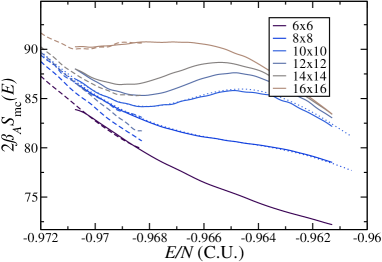
Figure 4: (Color online) The micro-canonical entropy as as a function of the energy in the system, obtained using the Wang-Landau method. The dashed, and solid curves show simulations in two different energy intervals; The dotted curves are simulations over a much larger energy interval.

We thus investigate the use broad histogram techniques; we first apply the one most widely reported in the literature, the Wang-Landau technique Wang and Landau (2001), which we have tested in quite a few variants. We find that the best way to represent the results is by using the micro-canonical entropy $d\ln g/dE$ versus $E$. From

$$\frac{d}{dE}P_{\beta}(E)=\frac{d}{dE}\left(g(E)e^{-\beta E}\right)=0,$$ (78)

we see that for an energy satisfying

$$2\beta_{A}d\ln g(E)/dE=\alpha_{B}(T)^{2}$$ (79)

we have an extremum of the probability density. When there is one solution this is the maximum; where there are multiple (as well shall see below, that usually means three) solutions we may have a first-order phase transition. Numerically the quality of the calculations can be slightly questionable, since we need to take a numerical derivative of the density of states. This latter quantity is obtained through a Monte Carlo technique, and thus has associated statistical errors, which are considerably amplified when taking derivatives, see the discussion in the Appendix. This means that we must impose a very high threshold to the convergence of the algorithm. As a consequence, we find questionable quality of the Wang-Landau results for system sizes beyond about 16 by 16, almost independent of the variant of the procedure we have applied, see Fig. 4. In that figure we see that we get good (but not perfect) overlap between the results in the various energy regions we have split the simulation in; we also see that $16\times 16$ is much flatter than all the other simulations, but needs better data to draw reliable conclusions.

The Wang-Landau procedure is different from a normal Monte Carlo procedure, since the acceptance criteria (i.e., the weights) change during a simulation. This means that it is difficult to run such simulations in parallel. Even if we could, the apparent long time scales associated with equilibration and phase coexistence suggest that we would rather use a method that only occasionally changes the Monte Carlo weights, such as the optimal energy diffusion (OED) algorithm we discuss in the previous section and in Appendix C.

Optimal Energy Diffusion results

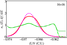
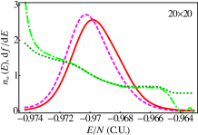
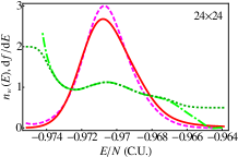
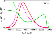
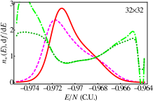
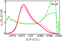
Figure 5: (Color online) Some typical results from optimal energy diffusion simulations. The plots differ in the value of $N=N_{x}\times N_{y}$ displayed in the top right-hand corner. In each plot, the solid red curve is a normalized probability histogram for walkers ($n_{w}(E)$), the dashed purple curve is (a smoothed version) of the derivative of positive direction walker density, $df/dE$. The light green curve shows the ratio between the red and purple curves, which should be one on convergence; the dark green curve gives a smoothed version of this ratio as described in the text, see Appendix C for the details. The difference between largest and smallest values of the red and purple curves is about 200 for the largest system size shown.

We show a typical result from one iteration of the OED algorithm in our implementation in Fig. 5. We see that we obtain reasonable convergence for the weights, and seem to have optimized the current well, since the two relevant curves ($n_{w}(E)$ and $df/dE$, see the discussion around Eq. (105) for details) almost coincide. The peak in these curves shows a pronounced minimum in energy diffusivity (typically the difference between largest and smallest values grows with system size, and is about 200 for the largest system size shown). As we go to larger system sizes, there seems to be a trend that is highly suggestive of the development of two peaks in the inverse diffusivity. If we link such peaks to features in the energy landscape that give rise to phase transitions, this might be the first indication of the pair of transitions predicted in the KTHNY picture.

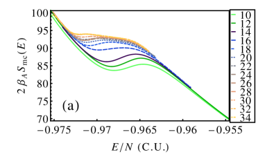
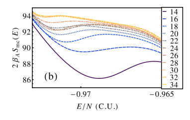
Figure 6: (Color online) The microcanonical entropy (the derivative of the logarithm of the density of states), as a function of the energy in the system. The values on the vertical axis have been scaled by $2\beta_{A}$ so that their values equal the value of $\alpha_{B}(T)^{2}$ that makes the probability density peak at the energy for each point. The label of each curve is $\sqrt{N}$. Figures (a) and (b) show the same data on different scales

We show the microcanonical entropy $S_{\text{mc}}(E)\equiv\frac{d}{dE}\ln g(E)$ for all simulations we have performed in Figs. 6. The advantage of that quantity, when expressed in natural energy units by multiplication of the energy by $2\beta_{A}$, is that it allows us to read off the value of $\alpha_{B}(T)^{2}$ that gives us the peak (or, in a few cases peaks) in the canonical probability at that energy directly from the graph. Having one intersection corresponds to a single peak of $P_{\beta}(E)$, and three intersections corresponds to two peaks and a minimum in between. As we can see the separation and depth of the peaks moves rapidly together – actually at the largest values of $\sqrt{N}$ it is debatable whether we even have three intersections (see also Fig. 12 below).

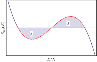
Figure 7: (Color online) The Maxwell construction for the microcanonical entropy. The red dashed line shows a typical finite size result, that is not convex. The best model of the large $N$ limit is obtained by a Maxwell construction, where the two parts cut from the entropy curve are of equal area $A$, and we thus get the solid blue curve as the best possible equation of state. The size of the cut areas, $A$, will naturally scale with $1/\sqrt{N}$ [and thus scales with $\sqrt{N}$ as a function of $E$], and provides us with a measure of the interface free energy.

Of course in the thermodynamic limit we cannot have multiple intersections. Since $S_{\text{mc}}$ is convex, the best approximation to the thermodynamic limit is obtained by a Maxwell construction, Fig. 7. Here we draw a straight line across the dip region, such that the area between the curves between the first to second intersection equals that between the second to third intersection. This area, suitably scaled, is actually just the interface free energy, which we expect to go to a non-zero constant if there is a first order transition. Since we plot $S_{\text{mc}}$ as a function of $E/N$, this would mean that the area on the graph scales like $1/\sqrt{N}$, and thus the interface free energy scaled with the interface length scales as $F_{S}/\sqrt{N}=A$, with $A>0$.

Interface free energy

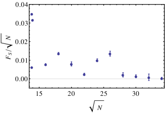
Figure 8: (Color online) Interface free energy per unit length as a function of the size of the system. The two additional high-lying points near $\sqrt{N}=14$ are $N_{x}\times N_{y}=16\times 12$ and $12\times 16$.

The behavior we find is quite different – we seem to be unable to extract a reliable trend for the interface free energy from the results as shown in Fig. 8. The results for the largest systems seem to suggest that the interface free-energy $A$ converges to zero, compatible with a total absence of a first order phase transition for the larger system sizes, but with substantial oscillatory behavior before that limit is reached. So the question is now: is there any evidence for a phase transition at all? The results shown in Fig. 5 suggest that there is one, and reasonably likely a second, bottleneck in energy diffusivity. Studies of the technique applied to spin models have shown that such results are usually linked with a phase transition – in most cases continuous transitions associated with diverging correlation lengths and their associated diverging timescales. We shall now argue that there is a clear indication that we have one and possibly two continuous phase transitions in the narrow energy range studied in Fig. 6.

Shear modulus and $C_{V}$

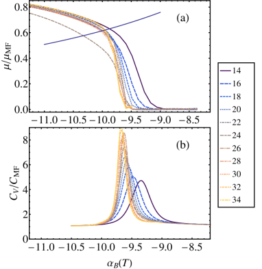
Figure 9: (Color online) (a) The value of the shear modulus $\mu$ divided by its mean-field value as a function of $\alpha_{B}(T)$ in the canonical ensemble. The solid blue line is the KT critical line, see Eq. (9) in Ref. Šášik and Stroud, 1994. The lowest $\alpha_{B}(T)$ results rely on an extrapolation of the data, partially using the crystalline density of state [Appendix D] (b) Specific heat divided by its mean-field value as a function of $\alpha_{B}(T)$ in the canonical ensemble. As usual Rosenstein and Li (2010) we make the approximation that all other temperature dependencies are replaced by $T_{c}^{\text{MF}}$.

The natural alternative to a first order phase transition is the KTHNY Kosterlitz and Thouless (1973); Halperin and Nelson (1978); Nelson and Halperin (1979); Young (1979) scenario. The normal liquid to hexatic transition is supposed to be in the universality class of the Kosterlitz-Thouless (KT) transition of the XY model and is associated with the binding of the free disclinations. In order to show a comparison with the classical picture of such transitions, we have used our results, reported later in this paper, to obtain the specific heat in the canonical ensemble, see Fig. 9. There is a peak in the specific heat which seems to grow with the number of vortices. This is rather similar to what can be seen for the XY modelVan Himbergen and Chakravarty (1981), but from the data it is unclear whether the peak in the specific heat saturates with $N$ – as it does for the XY model – or continues to grow (as it would if the transition were first order as discussed in, e.g., Refs. Janke, 1990; Bittner and Janke, 2005. Another striking feature of the specific heat is that the region associated with the peak is small and there seem to be no noticeable precursors of it on the high-temperature side of the transition. It seems to spring up from nowhere. The critical region in $\alpha_{B}(T)$ associated with the hexatic transition seems to be very narrow. The entropy in this peak, obtained by subtracting the mean-field contribution and integrating over $\alpha_{B}(T)$ seems to be almost independent of system size and is plotted in Fig. 10a. We calculate the entropy in the approximation

$$\delta S=\int_{T_{0}}^{T_{1}}(C_{V}-C_{MF})/\alpha_{B}(T_{c}^{\text{MF}})d\alpha_{B}(T).$$ (80)

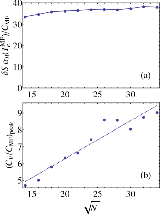
Figure 10: (Color online) Entropy (a) and peak height (b) contained in the “peak” of the specific heat relative to a mean-field crystal background. As usual Rosenstein and Li (2010) we make the approximation that all other temperature dependencies apart from $\alpha_{B}(T)$ are replaced by $T_{c}^{\text{MF}}$.

The value of the specific heat at its peak shows conflicting trends (see Fig. 10b) as a function of system size. For the smaller systems the peak height increases roughly as $\sqrt{N}$. Such rapid growth is more characteristic of a system undergoing a first-order phase transition. Indeed if we only had data up to $\sqrt{N}\leq 26$ (see below for further discussions of this point) then we might have concluded that there was a genuine first order transition. But at the larger system sizes studied there is evidence that the growth in the specific heat has stopped its rise with $\sqrt{N}$ and is saturating to a finite value, which is the expected behavior at the XY transition.

The other signature of KT transitions are jumps in a modulus from zero to a finite value at the transitionŠášik and Stroud (1994). In Fig. 9a data for the shear modulus is displayed. The (universal) jump from zero to a finite value as the temperature is reduced through the hexatic phase into the crystalline phase arises when the free dislocations in the hexatic liquid bind together. Apart from the case $N=24\times 24$ (see below for discussion of this case), we see the expected convergence to a finite value at the critical point and to zero on the high temperature side of the phase transition.

Maxwell analysis

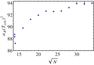
Figure 11: (Color online) A plot of the parameter $\alpha_{B}(T_{\text{crit}})^{2}$ for the temperature $T_{\text{crit}}$ where the two peaks in $P_{\beta}(E)$ are of identical height.

Now we have found some evidence that suggests the KTHNY scenario might apply, let us analyze the Maxwell construction a little further. In Fig. 11 we have plotted the critical value of $\alpha_{B}(T)$ where the two peaks in $P_{\beta}(E)$ are of the same height. But there is more striking behavior of the intersection points determined in the Maxwell construction and its uncertainty plotted in Fig. 12. The width of the Maxwell construction shrinks rapidly (possibly to zero) with increasing $N$. This is not what would be expected for a genuine first order phase transition, as seen for instance in hard-disk systems Bernard and Krauth (2011). One would have expected the width to saturate to the energy difference between the liquid and crystal states.

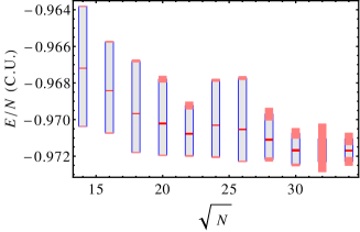
Figure 12: (Color online) Representation of the full range of the Maxwell construction , with the midpoints and uncertainty (red); full range (blue) and endpoints with range of uncertainty as an orange bar.

Extrapolation

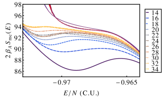
Figure 13: (Color online) Similar to Fig. 6b, with two naive $[1/1]$ Padé extrapolations [see main text for details] to $N\rightarrow\infty$ (one including all data from $N=14^{2}$ and up, the other from $N=16^{2}$ and up). The width of the extrapolated curves is a measure of the uncertainty, obtained by excluding the case $N=34^{2}$.

One way to try and gain an understanding of the thermodynamic limit of the entropy is by an approximate extrapolation. A naive extrapolation using a $[1/1]$ Padé approximant,

$$S_{\text{mc}}(E,\sqrt{N})=(a(E)+b(E)/\sqrt{N})/(1+c(E)/\sqrt{N}),$$ (81)

fitted to the entropy curves, as in Fig. 13, shows again that even though the set of curves is too limited to completely determine the density of states in the phase transition region, a trend can nevertheless be seen there. For lower energies (and for higher ones as well, but we show no results here) the extrapolation is actually quite stable. Also, the results of a $[2/2]$ extrapolation do not look appreciably different.

Understanding nonuniversal behavior

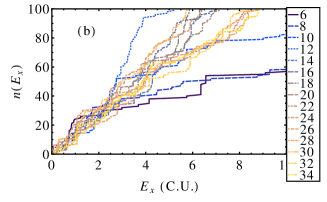
Figure 14: (Color online) The number of crystalline states below the excitation energy $E_{x}$ on a torus of $\sqrt{N}l_{B}$ by $\sqrt{3N}l_{B}/2$ for various values of $\sqrt{N}$. (a) shows the data as a function of the excitation energy per particle $E_{x}/N$ over a wide range; (b) shows the results as a function of $E_{x}$, which enters the Boltzmann factor.

One of the questions we need to ask ourselves, is why does the process of increasing $N$ lead to such large changes in the apparent nature of the phase transition from one size to the next as seen, e.g., in Fig. 12. These differences we believe have a topological origin, and are related to the occurrence of degenerate ground states, which have some influence on the results. We now solve the Diophantine equations (41) with the help of Mathematica, see Fig. 14.

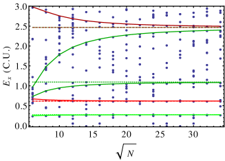
Figure 15: (Color online) Excitation energy of lowest energy crystalline states as a function of the number of vortices. The solid green and solid red lines connect excitations in two families that described small deformations of the triangular crystal; the dashed line are the thermodynamic limit of these energies.

	$14\times 14$	$16\times 16$
more liquid
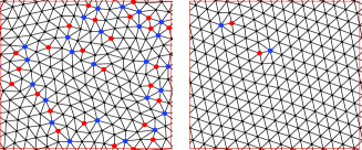
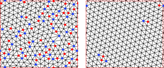
more crystalline

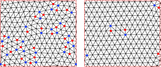
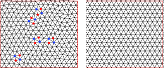
Figure 16: (Color online) Snapshots and steepest descent minimization: a few typical examples. Left column for $14\times 14$ vortices, right $16\times 16$. The top row is at a slightly higher energy (more liquid like). Each pair of pictures shows two related Delaunay diagrams of the vortex lattice. The left picture is a direct image from a snapshot (a single configuration in a simulation); the right picture is the result from a steepest descent minimization based on the snapshot. In each case a red dot shows 5-fold coordination, a blue dot 7-fold.

The picture that emerges seems rather complex. We see a density of states that roughly increases with system size, but there are obvious exceptions. The low-energy spectrum, which is the only part with any relevance to the simulations, is highly complex. The most telling analysis is shown in Fig. 15. There we see that for $\sqrt{N}=14,26,28$ we have a degenerate ground state (actually, since the additional groundstates come in pairs inequivalent under reflection, the degeneracy is three). The neighboring points, $\sqrt{N}=12,16,24,30$ have exceptionally low energy states ($E_{x}=0.065$ and $0.066\ \text{C.U.}$ for $\sqrt{N}=12$, $0.071$ for $\sqrt{N}=16$, $0.067$ for $\sqrt{N}=24$, and $0.070$ for for $\sqrt{N}=30$, respectively) that almost behave like an additional ground state. For $\sqrt{N}=26$ we have both a degenerate ground state, and a close-by set of states at $E_{x}=0.067$ and $0.070\ \text{C.U.}$. The green and red solid lines in Fig. 15 connect families of states that describe small deformations of the original equilateral lattice (the dashed lines shows the large-$N$ limit). If we restrict ourselves to the case $N_{x}=N_{y}=\sqrt{N}$, we find that in this limit these typical excitations energies are given by

$$E=-N+\delta_{i}\,k^{2},$$ (82)

with $k=1,2,\ldots$ and $\delta_{1}=0.274$ and $\delta_{2}=9/4\,\delta_{1}$. (These are the horizontal dashed lines in Fig. 15). Also note the enormous growth in the number density of crystalline states as $N$ increases revealed in Fig. 14.

Defects

One of the very important aspects of the KTHNY mechanism is the role of defects, and their (un)binding. Early on in our work, we decided to look at the topological nature of some of the states in the simulations, by looking at configurations (snapshots), and letting these relax through a steepest descent minimization to determine better their topological content. We produced a Delaunay triangulation to examine the topological content of the states. In Fig. 16, we present a few interesting examples of this work. The snapshots themselves mainly show grain boundaries, apart from the lowest energy $16\times 16$ picture, which shows bound defect pairs. What we see in the crashes is rather typical: we have a “misaligned crystal” due to a few bound defect pairs.

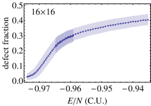
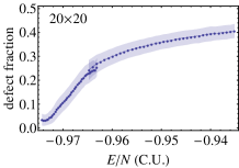
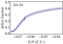
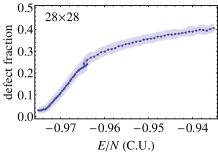
Figure 17: (Color online) Density of defects, defined as the fraction of points in the Delaunay diagram without 6-fold coordination, as a function of energy per vortex $E/N$ for four different system sizes, labeled as $N_{x}\times N_{y}$. The width of each band is a measure for the standard deviation in the answers. There appears to be clear evidence that apart from at extremely low energies, where we may be seeing a sharp feature developing, the density of defects is largely independent of $N$. (Breaks in the lines are caused by overlaying two separate simulations).

As we shall explain below, we have done a large number of calculations of the vortex positions. Unfortunately, a visual analysis in terms of Delaunay diagrams is practically impossible, but one thing we can do is plot the density of defects (any point that is not 6-fold coordinated) as a function of energy, as in Fig. 17. We find a sharp fall at low energies in the simulations. The conclusion appears to be that for energies down to $E/N=-0.96$ the phase-diagram is dominated by grain boundaries; at lower energies we find (mostly bound) pairs of defects. There appears to be some (but rather insubstantial) evidence of a further potential phase transition at the lowest possible energies, $E/N<-0.97$.

Density-Density Correlations

$N=16^{2}$	$N=20^{2}$	$N=24^{2}$	$N=28^{2}$

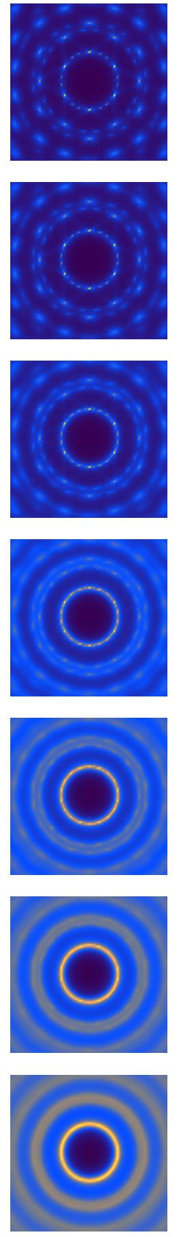
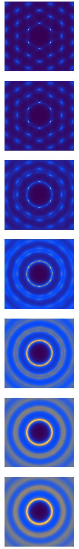
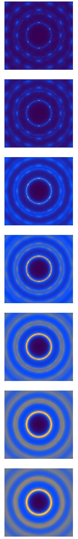
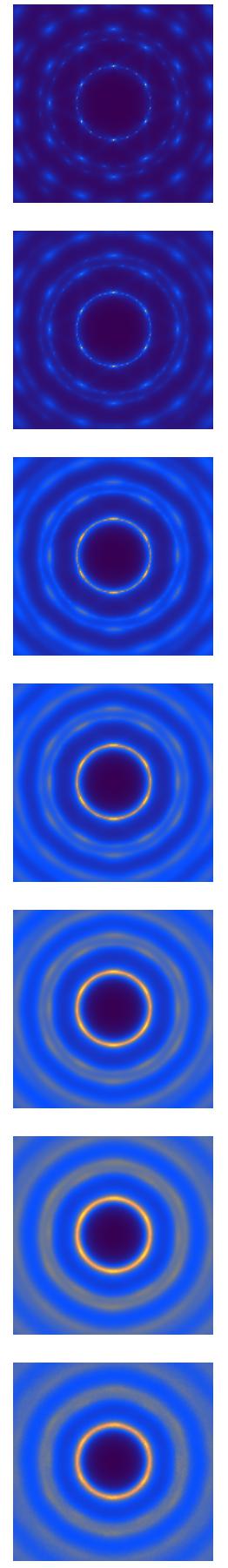
Figure 18: (Color online) Density-density correlation functions for four different system sizes ($16^{2}$, $20^{2}$, $24^{2}$, and $28^{2}$). The energy increases from top to bottom, but all values are in the flat region of the entropy curve (first row: $E/N=-0.9738$, second: $-0.9723$, third: $-0.9706$, fourth: $-0.9691$, fifth: $-0.9675$, sixth: $-0.9658$, and last row: $-0.9643$.)

A convenient measure for the extent of crystalline order in the liquid state can be obtained by the density-density correlations discussed in Sec. IV.1. We have plotted a few selected images for the four standard system sizes in Fig. 18. We see in that figure that as we increase the energy the system goes from a crystalline Bragg-like pattern to a typical liquid pattern with rotational invariance. The Bragg-like patterns will not consist of true delta function Bragg peaks because we can have only quasi-crystalline order in 2D systems according to the Mermin-Wagner theorem.

Notice the differences even at the lowest energies between $N=20^{2}$ and the other sizes. The other sizes are much less strongly modulated. This could be due to the fact that all of the other sizes in that figure have either an anomalously low-lying deformed crystalline state, or even a degenerate ground state. This could have important consequences for correlations at the lowest energies used in Fig. 3. But there are also other mechanisms at play which act to restore rotational invariance.

There is a competition between the ordering into the perfect low-energy structure(s) favored by the periodic boundary conditions and the misalignments induced by dislocations (bound $7-5$ defect pairs). The energy cost of defects can be partially balanced by the entropy gain from the large number of positions available for them. The width of the peaks in $P(E)$ in Fig. 3 shows that many types of defects could be present and as a consequence several mechanisms can be at work in restoring the rotational symmetry of the liquid state at the system sizes we can study. But at energies which correspond to the crystalline and hexatic states, the central ring is clearly being modulated, indicating that at these energies the defects have not yet fully restored the rotational invariance. For the hexatic state at least, one expects that in the thermodynamic limit there will be full rotational invariance; it is a liquid (see also Sec. VII).

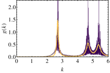
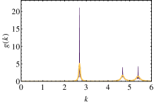
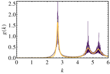
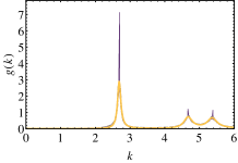
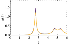
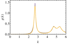
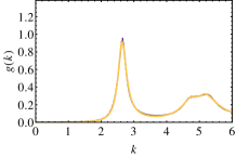
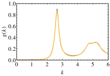
Figure 19: (Color online) Correlation length-sample evaluation for $N=26\times 26$, and energies (from top to bottom) $E/N=-0.974431$, $-0.971131$, $-0.967831$, $-0.964531$. The left column shows the angular average of the density-density correlations function; the right column shows the same for a narrow ray of width $\delta\theta=\pi/30$ about the crystalline axes. In each curve the thin dark purple curve is the data, and the thick orange curve is the result with a fit of a smoothed version of the data with a sum of Lorentzians multiplied with $k^{2}$ to take care of the correlation hole. Note that for the column at the right we use the width at the top, rather than the Lorentzian fit, to determine the correlation length.

Correlation lengths

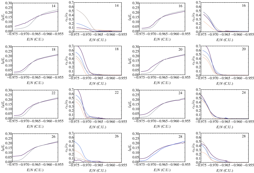
Figure 20: (Color online) Inverse crystalline correlation lengths (solid line: bulk and dashed line: on-axis) and “first-ring” Fourier components ($c_{6i}$: $i=1$ solid black, $i=2$: dashed gray, $i=3$: long-dashed blue, $i=4$: dotted orange).

We find it hard to extract a crystalline correlation length from the simulation data – especially near the crystalline states. If we collapse the data shown in Fig. 18 onto the radial axis by performing an angular integration – which in is just a sum over a finite number of grid points – we typically obtain data such as that shown in the left column of Fig. 19.

One approach which we use to extract a correlation length is to fit this data with a sum of Lorentzians, multiplied with a factor of $k^{2}$ to take into account the correlation hole. We then take the length scale for the inverse width of the lowest peak as an estimate of the crystalline correlation length. This choice seems rather obvious, but gives what is likely to be an overestimate of the width (and thus an underestimate of the correlation length) at energies at which the the rings are modulated. An alternative definition of the correlation length, would be to consider correlations only along (or very near) the three “natural” crystal axes, aligned with the simulation cell. We then fit a Lorentzian peak through 5 points at the top of the first peak of the correlation function, and we get a correlation length that is substantially larger at low energies than that obtained from the angular average, but rather similar at higher energy. We shall call this the “on-axis correlation length”, and use this as our preferred measure of a crystalline correlation length. Both definitions of the correlation length are plotted in Fig. 20.

Dependence of the correlation length on energy

We now can try to analyze the behavior of the correlation lengths as a function of energy. In the left column of Fig. 20 we see that the correlation lengths decrease quickly in the liquid as the energy $E/N$ increases, and behaves at the crystal end – very much like the behavior of the density of defects shown in Fig. 17. It once again shows three regions of behavior: liquid behavior, which we shall argue below is linear in energy; a sudden change at about $E/N=-0.965$, and a second change for $E/N\simeq-0.972$. This latter change is hard to interpret, because at that point the correlation length is much larger than the system size, as we can see more clearly in Figs. 21 and 22.

We have also examined the modulation of the first ring by constructing the Fourier analysis along the first ring of the density-density correlation function. In other words we have looked at the azimuthal intensity profile $I(\phi)=\sum_{n}c_{6n}\cos 6n\phi$; see Fig. 20. The modulation sets in around an energy $E/N\approx-0.965$, but the form it takes seems to be sensitive to the value of $\sqrt{N}$, indicating again that low-lying crystalline states might be playing a significant role.

Scaling analysis

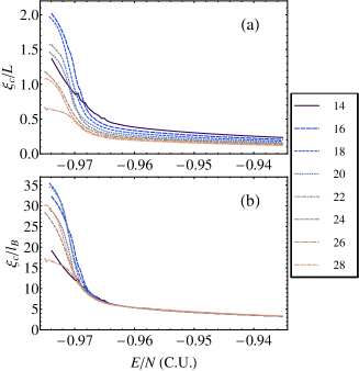
Figure 21: (Color online) Crystalline correlation lengths as a function of energy; (a): in units of the system size, $L=\sqrt{N}l_{B}$, (b): in units of the magnetic length $l_{B}$.

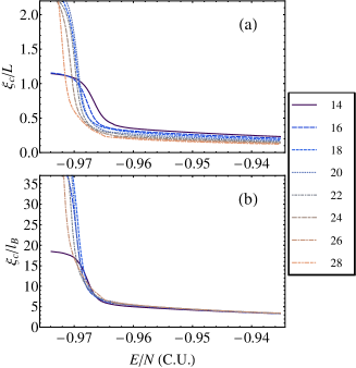
Figure 22: (Color online) On-axis crystalline correlation lengths as a function of energy; (a): in units of the system size, $L=\sqrt{N}l_{B}$, (b): in units of the magnetic length $l_{B}$.

One possible way to see whether there is any sign of a phase transition in the crystal data is to perform a scaling analysis, and plot the data as a function of the system size, taken as $L=\sqrt{N}l_{B}$. As we can see in Figs. 21 and 22 neither of the definitions scales as one would expect if there was a phase transition, when plots of $\xi_{c}/L$ should cross at the critical value of the energy.

We can perform a similar analysis for the hexatic correlation length. These are expensive to calculate, and we have thus limited the results to a few examples. In each case we have applied the contour finding and improvement method on the data for the order parameter field. Depending on energy, we had to reject between 15-25% of our results due to lack of or misidentification of (usually one) vortex, and there thus is a possibility of a bias in the data. From the positions we can through standard ways determine the hexatic correlation length (essentially, the width of the peak at $\boldsymbol{k}=0$.)

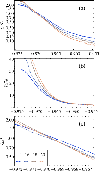
Figure 23: (Color online) Hexatic correlation lengths $\xi_{6}$ as a function of energy; (a): divided by $L=\sqrt{N}l_{B}$, (b): divided by the magnetic length $l_{B}$; (c) zooms in on the detail of the crossing in (a).

As we can see in Fig. 23, the hexatic correlation lengths do show some of the behavior expected for a phase transition between liquid and hexatic liquid, which is in the universality class of the XY model; they even cross at values of $\xi_{6}/L$ similar to those of the XY model. Clearly, we have not reached convergence and we would benefit from additional results for larger systems, which are unfortunately prohibitively computationally expensive.

Extrapolation from the liquid

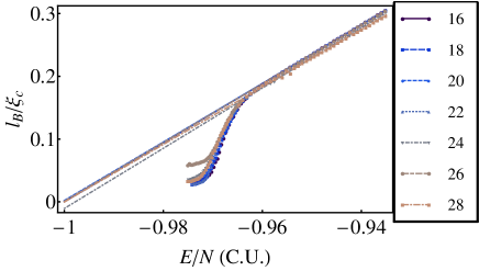
Figure 24: (Color online) Crystalline correlation lengths: Extrapolation of the liquid behavior. The symbols show the various data sets; the lines are the extrapolation from the higher energy part of the data.

It has been argued in the pastDodgson and Moore (1997); Lee and Moore (1994); O’Neill and Moore (1992) that the liquid might persist all the way down to zero temperature, when it forms the Abrikosov crystal. If we extrapolate the inverse correlation length $l_{B}/\xi_{c}$ in the liquid regime (which seem to satisfy a naive linear relation $l_{B}/\xi_{c}=c(E/N-E_{0})$), we find that all bar one of the cases extrapolate with $E_{0}=-1$ – and that the one exceptional case (at $\sqrt{N}=24$) is still close, see Fig. 24. The simulation data at the lower energies deviate rather strongly from the fit, showing a change of behavior for an energy around $E/N=-0.965$, presumably due to the transition to the hexatic phase. In the earlier simulations on the sphere the correlation length was found to grow as $\xi_{c}\sim|\alpha_{B}(T)|l_{B}$ within the canonical ensemble. Alas, we cannot confirm this result as we only collected data in the microcanonical ensemble over the energy range close to the transitions, but the results might be consistent with such a growth of $\xi_{c}$, at least until the topological defects start to bind. Notice that departures from the linear relation set in rather sharply, indicating that the critical region of the hexatic transition is small.

Shear Modulus (microcanonical)

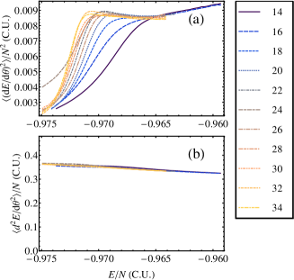
Figure 25: (Color online) The micro-canonical ingredients to the calculation of the shear modulus as a function of energy, for values of $\sqrt{N}$ from $14$ to $34$. In (a) we show the shear susceptibility, in (b) the shear stiffness.

In Fig. 25 we show the microcanonical ingredients that enter the calculation of the shear modulus. Clearly all of the structure in the shear modulus is caused by the shear susceptibility $\langle(dE/d\theta)^{2}\rangle$. Its behavior is once again suggestive of two places of changing behavior. The first change of behavior occurs again at $E/N\approx-0.965$, where the slope of the curve changes sign; the second change occurs at energy probably below $E/N=-0.9715$, where we see a sharp drop, and a change to crystalline behavior (where the shear susceptibility decays to zero). The first of these changes is much smoother than the second.

VII Discussion and Conclusions

Our main conclusion is that the old simulational evidence for a first order phase transition to the crystal state from the vortex liquid state is just an artifact of the rather small system sizes which were previously studied. The evidence for this statement is contained in Fig. 8. If we had only studied sizes up to $\sqrt{N}=26$, there would have been good evidence for a first order transition. However, the interface free energy shown in Fig. 8 collapses towards zero for larger systems, implying that the transition is just not first-order.

The apparent first-order transition reported in earlier numerical studies with quasi-periodic boundary conditions Kato and Nagaosa (1993, 1993); Hu et al. (1994); Šášik and Stroud (1994); Šášik et al. (1995); Li and Nattermann (2003) is, we suspect, both a finite size effect and a consequence of the use of periodic boundary conditions. When the vortices move on the surface of a sphere there was no evidence of a first-order transition Dodgson and Moore (1997); Lee and Moore (1994); O’Neill and Moore (1992). We now suspect that the transition between crystal and hexatic liquid is continuous, and this will occur according to the KTHNY picture when the bound dislocations in the crystalline state unbind. However, for quasi-periodic boundary conditions the system can prematurely lower its energy by going to the crystalline state (probably by an amount not of order $N$ but just of magnitude $k_{B}T^{\text{MF}}_{c}\alpha_{B}(T)^{2}$, see Eq.(82)), and this small amount of energy is sufficient to upset the delicate balance of free energies of liquid and crystal and produce the apparent first-order transition, seen for small systems. It is an interesting question which set of boundary conditions, quasi-periodic or spherical, converges to the thermodynamic limit faster, but the evidence of this paper is that at least in the liquid regime, spherical boundary conditions might have the advantage.

In the KTHNY scenario there should be two transitions: The first is the one from a normal liquid to an hexatic liquid phase, and the second transition is that from the hexatic liquid to the crystal. We believe that we have strong evidence for the liquid-hexatic transition, see Fig. 23. The crossing of the curves of $\xi_{6}/L$ occurs just as would be expected for a transition in the XY universality class. Alas, the equivalent curves of $\xi_{c}/L$ for the hexatic to crystal transition fail to show a similar crossing. This is at least partially due to the magnitude of the crystalline correlations for low energies, which substantially exceed the system size. Fortunately the shear modulus (see Fig. 25a), provides strong evidence for the expected jump in its value at the transition.

We suspect that the failure to see crossing of the plots of $\xi_{c}/L$ is another consequence of finite size effects, which are very noticeable in the hexatic phase. The density-density correlations as shown in Fig. 18 depends on the orientation of $\boldsymbol{q}$ with respect to the boundaries of the simulational cell and a detailed examination of this modulation is given in Fig. 20. In the hexatic phase Peterson and KagenerPeterson and Kaganer (1994) showed that will be no such modulation in the thermodynamic limit. They derived a formula for the length scale $L^{*}$ which, for sizes $L>L^{*}$, the modulation will disappear. In our notation $L^{*}\sim\xi_{c}\exp[c\alpha_{B}(T)^{2}]$, but the numerical constant $c$ is not known. The results in Figs. 18 and 20 indicate that in our studies of the hexatic phase we have not reached this limit and that therefore finite size effects might still play a significant role.

Taking all of the evidence together we estimate the crystal to hexatic transition to be at $E/N=-0.9725\pm 0.0005\text{ C.U.}$ and the hexatic to normal liquid one at $E/N=-0.9645\pm 0.0005\text{ C.U.}$. The latter corresponds to $\alpha_{B}(T_{hl})\approx-9.5$, in agreement with our calculations of the canonical specific heat and shear modulus. We can only put an upper bound on the hexatic to crystal value, $\alpha_{B}(T_{ch})<-9.7$.

One striking feature of our simulations is the pronounced but narrow peak in the specific heat seen in Fig. 10. Given its prominence, it is surprising that experiments like that of Urbach et al.Urbach et al. (1992) failed to see it. We would urge further experiments to understand this discrepancy, which we are inclined to attribute to variations in the thickness of their films, which would tend to smear out the peak in the specific heat.

Finally we make a comment on the Monte Carlo simulations. It is a tacit assumption of simulation that the sizes one can reach are sufficiently large that one can make useful statements about what happens in the thermodynamic limit. The old simulations with periodic boundary conditions were mainly done for $\sqrt{N}\leq 16$ and so were naturally reported as providing evidence for a first order transition. They could not anticipate the trend which sets in for $\sqrt{N}>26$. By the same token, large finite size effects are clearly still present in our work, and going to larger values of $N$ might still conceivably produce a different story. We already have substantially improved upon the sizes which were previously studied, not only by using better computers, but mainly by a better algorithm. Without the adoption of the optimal energy diffusion algorithm we would never have been able to converge the simulations. The main bottleneck to increasing the size of the system being simulated is the barrier to energy diffusion. So in order to do such simulations a better algorithm will have to be considered. We believe the most likely place improvements could be made is in the basic Monte Carlo step, but we have no alternative to propose at this stage.

Appendix A Quartic terms in the interactions

To calculate the quartic interaction terms in the Ginzburg-Landau functional we need to calculate the integral of $|\Psi|^{4}$ over the simulational cell. We again expand in the basis (10). First we integrate over $y$,

$$\int_{0}^{L_{y}}dy\,g_{j_{1},s_{1}}^{*}(y)g_{j_{2},s_{2}}^{*}(y)g_{j_{3},s_{3}}(y)g_{j_{4},s_{4}}(y)=\frac{1}{L_{y}}\delta_{j_{1}+j_{2}+N(s_{1}+s_{2}),j_{3}+j_{4}+N(s_{3}+s_{4})}\,,$$ (83)

and then simplify the calculation over $x$ using the Kronecker delta from the $y$ integral above to

$$\int_{0}^{L_{x}}dx\,f_{j_{1},s_{1}}^{*}(x)f_{j_{2},s_{2}}^{*}(x)f_{j_{3},s_{3}}(x)f_{j_{4},s_{4}}(x)=\frac{e^{-\frac{4\pi\left(n_{p_{1}}^{2}+n_{p_{2}}^{2}\right)}{\sqrt{3}N_{y}^{2}}}}{\pi l_{B}^{2}}\int_{0}^{L_{x}}dx\,\exp\left(-\frac{2N_{x}^{2}}{\sqrt{3}\pi N^{2}}\left(\theta_{y}+2\pi(n_{s}-Nx/L_{x})\right)^{2}\right),$$ (84)

where

$$n_{p_{1}} =j_{1}-j_{2}+N(s_{1}-s_{2}),$$

$$n_{p_{2}} =j_{3}-j_{4}+N(s_{3}-s_{4}),$$

$$2n_{s} =j_{1}+j_{2}+j_{3}+j_{4}+N(s_{1}+s_{2}+s_{3}+s_{4})=2(j_{1}+j_{2}+N(s_{1}+s_{2})).$$ (85)

We now perform the sum over the variables $s_{i}$ which is required in each of the basis functions, see Eq. (10). Changing the summation over $s_{i}$ to the variables $s_{p_{1}}$, $s_{p_{2}}$ and $s_{s}$, where we write

$$n_{\alpha}=\left\lfloor n_{\alpha}\right\rfloor+2Ns_{\alpha}$$ (86)

and $\left\lfloor n_{\alpha}\right\rfloor$ is an integer ranging from $0$ to $2N-1$, and the label $\alpha=p_{1},p_{2},s$. The variables $s_{\alpha}$ are three independent integers. We also see that $n_{p_{1}}$, $n_{p_{2}}$, $n_{s}$ are all integers, and that their pairwise sums must all be even. If we now perform the sum over $s_{s}$ in the expression (84), we find that we can write

$$\sum_{s_{s}=-\infty}^{\infty}\int_{0}^{L_{x}}dx\,f_{j_{1},s_{1}}^{*}(x)f_{j_{2},s_{2}}^{*}(x)f_{j_{3},s_{3}}(x)f_{j_{4},s_{4}}(x) =\frac{e^{-\frac{\pi\left(n_{p_{1}}^{2}+n_{p_{2}}^{2}\right)}{\sqrt{3}N_{y}^{2}}}}{\pi l_{B}^{2}}L_{x}\int_{-\infty}^{\infty}d\xi\,\exp\left(-\frac{2N_{x}^{2}}{\sqrt{3}\pi N^{2}}\left(\theta_{y}+2\pi(\left\lceil n_{s}\right\rceil-N\xi)\right)^{2}\right)$$

$$=\frac{e^{-\frac{\pi\left(n_{p_{1}}^{2}+n_{p_{2}}^{2}\right)}{\sqrt{3}N_{y}^{2}}}}{\pi l_{B}^{2}}\sqrt{\frac{\pi}{2}}l_{B}=\frac{e^{-\frac{\pi n_{p_{1}}^{2}}{\sqrt{3}N_{y}^{2}}}e^{-\frac{4\pi n_{p_{2}}^{2}}{\sqrt{3}N_{y}^{2}}}}{\sqrt{2\pi}l_{B}}.$$ (87)

Taking all of this together we get

$$\int dxdy\,\phi_{j_{1}}^{*}(x,y)\phi_{j_{2}}^{*}(x,y)\phi_{j_{3}}(x,y)\phi_{j_{4}}(x,y)\\ =\delta_{\left\lceil j_{1}+j_{2}-j_{3}-j_{4}\right\rceil,0}\sum_{s_{p_{1}}s_{p_{2}}=-\infty}^{\infty}\frac{e^{-\frac{4\pi\left(\left\lceil n_{p_{1}}\right\rceil+2Ns_{p_{1}}\right)^{2}}{\sqrt{3}N_{y}^{2}}}e^{-\frac{4\pi\left(\left\lceil n_{p_{2}}\right\rceil+2Ns_{p_{2}}\right)^{2}}{\sqrt{3}N_{y}^{2}}}}{\sqrt{2}\sqrt[4]{3}\pi l_{B}^{2}N_{y}}\\ =\delta_{\left\lceil j_{1}+j_{2}-j_{3}-j_{4}\right\rceil,0}\frac{\sqrt[4]{3}N_{y}}{4\sqrt{2}\pi l_{B}^{2}N^{2}}\theta_{3}\left(\frac{n_{p_{1}}\pi}{2N}\middle|e^{-\frac{\sqrt{3}N_{y}^{2}\pi}{4N^{2}}}\right)\theta_{3}\left(\frac{n_{p_{2}}\pi}{2N}\middle|e^{-\frac{\sqrt{3}N_{y}^{2}\pi}{4N^{2}}}\right).$$ (88)

The quartic term in the GL free energy is given by

$$E_{4}(\{c\}) =\frac{\pi^{2}}{2^{5/2}3^{1/4}\text{ }N_{y}}\sum_{n_{s}=0}^{2N-1}\left|\sum_{n_{p}=0}^{2N-1}\delta_{n_{s}+n_{p},\text{even}}\left[\sum_{s_{p}=-\infty}^{\infty}e^{-\frac{\pi(n_{p}+Ns_{p})^{2}}{\sqrt{3}N_{y}^{2}}}\right]c_{\left\lceil(n_{p}+n_{s})/2\right\rceil}c_{\left\lceil(n_{p}-n_{s})/2\right\rceil}\right|^{2}$$

$$=\frac{\pi^{2}}{2^{5/2}3^{1/4}\text{ }N_{y}}\sum_{n_{s}=0}^{2N-1}\left|Q_{n_{s}}\right|^{2}.$$ (89)

Here $Q_{n_{s}}$ is as given in Eq. (27).

A.1 Shear Modulus

To calculate the shear modulus we need to calculate the $\theta$ dependent energy. We expand in the basis Eq. (71). The $y$ integral gives the usual Kronecker delta, and it is really straightforward to show that the quadratic term in the energy is unchanged, whereas in the quartic term we can use the technique shown above to find

$$\sum_{s_{s}=-\infty}^{\infty}\int_{0}^{L_{x}}dx\,f_{j_{1},s_{1}}^{*}(x,\theta)f_{j_{2},s_{2}}^{*}(x,\theta)f_{j_{3},s_{3}}(x,\theta)f_{j_{4},s_{4}}(x,\theta) =\frac{e^{-\frac{(\pi-i\tan\theta/2)n_{p_{1}}^{2}}{\sqrt{3}N_{y}^{2}}}e^{-\frac{(\pi+i\tan\theta/2)n_{p_{2}}^{2}}{\sqrt{3}N_{y}^{2}}}}{\sqrt{2\pi}l_{B}}.$$ (90)

Thus the quartic term in the energy is as given in Eqs. (72,73).

Appendix B Evaluation of density-density correlation function

Here we evaluate the density-density correlation function. We start from

$$g(\boldsymbol{q)} \equiv\int d^{2}r\,d^{2}r^{\prime}e^{i\boldsymbol{q}.(\boldsymbol{r}-\boldsymbol{r}^{\prime})}$$

$$\quad\times\left[\left\langle\left|\Psi(r)\right|^{2}\left|\Psi(r^{\prime})\right|^{2}\right\rangle-\left\langle\left|\Psi(r)\right|^{2}\right\rangle\left\langle\left|\Psi(r^{\prime})\right|^{2}\right\rangle\right]/\mathcal{N}^{4}$$

$$=\left\langle\left|\rho(\boldsymbol{q})\right|^{2}\right\rangle-\left|\left\langle\rho(\boldsymbol{q})\right\rangle\right|^{2},$$ (91)

with

$$\rho(\boldsymbol{q}) =\left\langle\int d^{2}r|\Psi(r)|^{2}e^{i\boldsymbol{q}\cdot\boldsymbol{r}}\right\rangle/\mathcal{N}^{2}.$$ (92)

We now multiply by the normalization constant squared, since we are only interested in the relative magnitude of correlations. We now evaluate $\rho(\boldsymbol{q})$. We choose

$$q_{y}=k_{y}/l_{B}=m_{y}2\pi/L_{y}=\frac{2\sqrt{\pi}m_{y}}{\sqrt[4]{3}l_{B}N_{y}},$$ (93)

and find that that the $y$-integral in this quantity can easily be evaluated as

$$\int_{0}^{L_{y}}dy\,e^{iq_{y}y}g_{j_{1},s_{1}}(y)^{*}g_{j_{2}s_{2}}(y)=\delta_{n_{1}-n_{2},n_{y}}=\delta_{n_{p},m_{y}},$$ (94)

where $n_{i}=j_{i}+Ns_{i}$ is the “unrestricted” summation variable. Once again we can replace the summation variables by $n_{p}=n_{1}-n_{2}$, $n_{s}=n_{1}+n_{2}$.

This is also helpful with the $x$-integral, which can now be rewritten as

$$\int_{0}^{1}dt\,\frac{2N_{x}\exp\left(-\frac{4\pi\left(n_{p}^{2}/4+(n_{s}/2-Nt)^{2}\right)}{\sqrt{3}N_{y}^{2}}+\frac{2i\sqrt{\pi}lN_{x}q_{x}t}{\sqrt[4]{3}}\right)}{\sqrt[4]{3}},$$ (95)

where $t=x/L_{x}$. We still need to sum this result over all $n_{s}$; we write $n_{s}=j_{s}+N_{x}N_{y}s_{s}$, (where $j_{s}$ is still half-integral, but $s_{s}$ is integer) and sum over all $s_{s}$. Using the fact that we can combine $t$ with each $s_{s}$, which we can rewrite as a shift in the integration boundaries by $s_{s}$, we find we can replace the sum over $s_{s}$ with a change in the integration boundaries to

$$\int_{-\infty}^{\infty}dt\,\frac{2N_{x}\exp\left(-\frac{4\pi\left(n_{p}^{2}/4+(j_{s}/2-Nt)^{2}\right)}{\sqrt{3}N_{y}^{2}}+\frac{2i\sqrt{\pi}lN_{x}q_{x}t}{\sqrt[4]{3}}\right)}{\sqrt[4]{3}},$$ (96)

with

$$q_{x}=k_{x}/l_{B}=2\pi m_{x}/L_{x}=\frac{\sqrt[4]{3}\sqrt{\pi}m_{x}}{l_{B}N_{x}}.$$ (97)

The result of this integral is

$$\exp\left(\frac{i\pi j_{s}m_{x}}{N_{x}N_{y}}-\frac{\sqrt{3}\pi m_{x}^{2}}{4N_{x}^{2}}-\frac{4\pi n_{p}^{2}}{\sqrt{3}N_{y}^{2}}\right).$$

Now combining $x$ and $y$ integrals with the coefficients in expansion of the wave function

$$\rho(\boldsymbol{q}) = \sum_{j_{s}=0}^{2N-1}c_{\left\lceil\left(j_{s}+n_{y}\right)/2\right\rceil}^{*}c_{\left\lceil\left(j_{s}-n_{y}\right)/2\right\rceil}$$ (98)

$$\quad\times\exp\left(-\frac{\sqrt{3}\pi m_{x}^{2}}{4N_{x}^{2}}-\frac{\pi m_{y}^{2}}{\sqrt{3}N_{y}^{2}}\right)\exp\left(\frac{i\pi m_{x}j_{s}}{N}\right)$$

$$= \exp\left(-\frac{1}{4}\left(k_{x}{}^{2}+k_{y}{}^{2}\right)\right)$$

$$\times\sum_{j^{\prime}=0}^{N-1}c_{j^{\prime}}c_{\left\lceil j^{\prime}+m_{y}\right\rceil}^{*}\exp\left(\frac{2i\pi m_{x}(j^{\prime}+m_{y}/2)}{N}\right)$$

$$= \exp\left(-\frac{1}{4}\left(k_{x}{}^{2}+k_{y}{}^{2}\right)\right)\exp\left(\frac{ik_{x}k_{y}}{2}\right)$$

$$\times\sum_{j^{\prime}=0}^{N-1}\left(c_{j^{\prime}}\exp\left(\frac{2i\pi m_{x}j^{\prime}}{N}\right)\right)c_{\left\lceil j^{\prime}+n_{y}\right\rceil}^{*}.$$

Appendix C Monte Carlo techniques

C.1 “Normal” Monte Carlo Calculations

C.1.1 Prior art

The classical way to tackle the problem at hand has been to use a standard Metropolis algorithm to sample the free energy at a given value of $\alpha_{B}(T)^{2}$, which plays a role similar to the usual $\beta$ parameter in statistical physics problems. Such techniques rely on a probabilistic acceptance criterion for a “move” between two configurations, which is usually of the bi-local form

$$P(E\rightarrow E^{\prime})=\min\left(1,w(E^{\prime})/w(E)\right).$$ (99)

The standard form is to use the Boltzmann factor,

$$w(E)=e^{-\beta E},$$ (100)

or in our case

$$w(F)=e^{-F_{GL}/k_{B}T_{c}^{MF}}.$$ (101)

Simulations of such a nature Kato and Nagaosa (1993, 1993); Hu et al. (1994); Šášik and Stroud (1994); Šášik et al. (1995); Li and Nattermann (2003) usually find that in a certain range of “inverse temperatures” $\alpha_{B}(T)$ – with our definition of the coupling strength $-10\lessapprox\alpha_{B}(T)\lessapprox-9$ – where we find coexistence of long lived states.

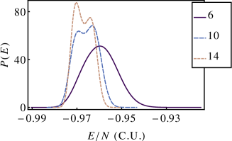
Figure 26: (Color online) A plot of the energy probability distribution near phase coexistence for Metropolis Monte Carlo simulations for systems containing $6^{2}$, $10^{2}$ and $14^{2}$ vortices.

For a given temperature, it is instructive to look at the distribution of energies contributing at that temperature. A typical example is shown in Fig. 26, where we see the double peak structure which is taken to be indicative of a first order phase transition. We can understand this as follows: We rewrite the partition function as an integral over a probability that the system has energy $E$,

$$Z(\beta)=\left\langle e^{-\beta E}\right\rangle=\int dE\,g(E)\,e^{-\beta E}=\int dE\,P_{\beta}(E).$$

This function $P_{\beta}(E)$ has extrema at an energy where the microcanonical entropy takes the value $\beta$,

$$S_{\text{mc}}(E)=\frac{d}{dE}\ln g(E)=\beta.$$ (102)

In the thermodynamic limit a first order phase transition thus occurs when there is a range of energies that satisfies (102), i.e., $S_{\text{mc}}(E)$ has a flat region. It is well-known that this not what is seen in finite system: In the finite size precursor we see a change in the slope of $S_{\text{mc}}(E)$ from negative to positive for a sort while, violating the convexity rules $S$ must satisfy in the thermodynamic limit. This gives rise to three intersections, corresponding to the two maxima and one minimum we see in Fig. 26. The best approximation of the convex thermodynamic limit can then be obtained from a Maxwell-type construction, where we replace the curve by a flat segment, for which the area above and below the curve must be equal, see Fig. 7. The size of this area is an estimate for the interface free energy for the first order phase transition, and since this is related to the area of the interface between the two phases, it should grow for two dimensions as the linear dimension of the system.

C.2 Broad histogram techniques

There are various broad-histogram techniques that sample the energy landscape directly Wang and Landau (2001); Trebst et al. (2004). An advantage of these is that we are able to get a more detailed view of the density of states, which reflects the nature of any phase transition more directly. In this work we concentrate on two such methods, the Wang-Landau techniqueWang and Landau (2001) and its variations and the Optimal Energy Diffusion (OED) Method Trebst et al. (2004). Both of these methods describe the statistical physics in the microcanonical ensemble, where the Monte Carlo aspect is a random walk in energy–and potentially a few other degrees of freedom, a case which we shall not consider here. The diffusion through the energy landscape – which we can of course completely describe as a high-dimensional configuration space – we prefer to parametrize by a few collective coordinates, one of which is energy. This low-dimensional projection can have all the complications, such as caustics, etc., we know from the topology of such reductions.

In all cases we shall assume that the transition probability used in the random walk will be chosen to depend on the projection coordinate (energy) only. The broad histogram that is used in these methods is an energy histogram. In the case of a continuous problem, this is obtained by dividing the energy into bins. If the energy is bounded from both above and below we can use the full range of energies, even though that is not always efficient. If the energy of the system is not bounded, or if there are certain areas in the range of energies that deserve more attention, we can carve out a restricted interval, and only look at energies within it. There is a serious danger if we make such intervals too small, however: suppose there is an (important) energy barrier just above the interval of interest. In that case, we would not be sampling all states for the energies we are considering, and may obtain an incorrect estimate for the density of states.

C.2.1 Wang-Landau

In the Wang-Landau algorithm Wang and Landau (2001) and its variants the random walk is driven directly by the logarithm of the density of state – the attempt is made to make the sampled histogram flat in all the projected directions. It is very easy to convince oneself that this is the case if the acceptance probability is given by the inverse of the (best estimate of the) density of states itself, i.e., $w(E)=1/g_{\text{est}}(E)$. For the continuous system considered here – most of the initial applications were to systems with discrete energy spectra – we divide the range of the interesting energy into bins, and start with an estimate of the density of states. Then, when the random walk visits an energy in a given bin, we update the estimate of $g$ in that bin by a factor $f>1$,

$$\ln g_{\text{est}}\rightarrow\ln g_{\text{est}}+\ln f.$$ (103)

When the histogram, the number of times we have visited each energy bin is suitably flat, we reduce the factor

$$f\rightarrow\sqrt{f},$$ (104)

or a similar reduction by another suitably chosen power-law. When $f$ becomes very small, $g_{\text{est}}$ will have converged to $g$.

There are various refinements one can make to this process Wu et al. (2005); Reynal and Diep (2005); Morozov and Lin (2007); Belardinelli and Pereyra (2007); Cunha-Netto et al. (2008); Zhou and Su (2008). In general, it has been shown that more complex patterns of choosing $f$ can lead to faster convergence. Also, we can choose to divide up the energy range into many small intervals that are easier to deal with – but this suffers from the risk that there will be important barriers that we are not treating well, and must always fail for a sufficiently complex energy landscape.

It is believed that the end-to-end transmission time, the simulation-time it takes for the random walk to move form the lowest part of the energy space, or vice-versa, is an important measure of the likelihood of success of the simulation. As has been shown in Ref. Dayal et al., 2004 there can be a serious issue with this end-to-end tunneling rate in real systems, with substantial slowing down of the process if there are funnels or barriers in the problem. Also, the use of Eq. (103) precludes the use of standard parallelization techniques usually applied to Monte Carlo simulations, since we update $\rho_{\text{est}}$ continuously.

C.2.2 Optimal energy diffusion

In the optimal energy diffusion method, one tries to optimize the current of random walkers between two extremal points in energy space Trebst et al. (2004); Wu et al. (2005); Bauer et al. (2010), by first building a simple model of this diffusion process, and choosing optimal parameters based on that model. The extrema can be the real bounds on energy, or the bounds of an interesting region – this must of course always be the case for continuous systems with energy unbound from above. We create two populations of walkers, one moving from the lowest to highest energy, the other from highest to lowest; in practice as soon as a walker reaches its final target, it is converted to a walker going in the opposite direction. If we take this as starting a new walker, we see that this is effectively an absorbing boundary condition. Walkers reaching the opposite boundary, the one that does not correspond to their target, are simply “reflected”, and keep their label. We record the position at each walker in two variables, $n_{w\pm}(E)$, where the $+$($-$) indicates the walker was released from the maximal (minimal) energy. The simulation process is started by releasing a walker from the boundary (if the states are known) or by starting with a walker without a label, which is absorbed and restarted when it reaches a boundary.

We now define the fraction of the walkers diffusing from the upper boundary as

$$f(E)=\frac{n_{w+}(E)}{n_{w}(E)},\quad n_{w}(E)=n_{w+}(E)+n_{w-}(E).$$ (105)

Clearly $f(E_{\text{min}})=0$ and $f(E_{\text{max}})=1$. The basic premise of the method is that we can use the simple model that in steady state, where the current $j$ of walkers will be independent of energy, we have a diffusion process for the current of $+$ walkers (which is equal in magnitude but opposite in sign to the current of $-$ walkers) described by the local process

$$j=D(E)n_{w}(E)\frac{df}{dE},$$ (106)

where $D(E)$ is an unknown function describing the local energy diffusivity. The expression (106) is a model of the process based on insight from diffusion, but clearly has no deep justification.

If we now optimize the current of walkers by the method of Lagrange multipliers, we find that it is maximal when

$$n_{w\text{opt}}(E)=w_{\text{opt}}(E)g(E)=\frac{df_{\text{opt}}}{dE}\propto\frac{1}{\sqrt{D(E)}}.$$ (107)

We now wish to use a standard Metropolis dynamics to find the optimal solution, which we take as sampling with the optimal choice of the weights $w$. We start from an initial set of weights $w(E)$, and use a standard Metropolis simulation to evaluate

$$D(E)\propto\left(n_{w}(E)\frac{df}{dE}\right)^{-1},$$ (108)

using

$$\frac{n_{w\,\text{opt}}(E)}{n_{2}(E)}=\frac{w_{\text{opt}}(E)}{w(E)}\propto\frac{1}{n_{w}(E)}\frac{1}{\sqrt{D(E)}}\propto\sqrt{\frac{df/dE}{n_{w}(E)}},$$ (109)

we find that up to a constant an improved estimate for the weights should be given by

$$\ln w_{\text{opt}}(E)=\ln w(E)+\frac{1}{2}\ln\frac{df}{dE}-\frac{1}{2}\ln n_{w}(E).$$ (110)

Of course that relies on both the model and the linearity in all the parameters – neither of which are perfectly true.

Since the Metropolis algorithm only depends on ratios of $w$’s, we do not need to know the value of the constant. At the same time, we see that the corresponding best estimate is

$$\ln g(E)=-\ln w(E)+\ln n_{w}(E).$$ (111)

Evidence seems to suggest that this approach is very powerful indeed. One of its main advantages is that it is a standard Metropolis calculation, which can be computationally optimized in the normal way for such approaches, including parallelization. The Wang-Landau algorithm, where weights change while we are simulating is much harder to fine tune in such a way. Also, as we have also seen in our work one can get stable results with weights that are not perfectly optimal.

C.2.3 Implementation

Since we are particularly interested in the derivative of the density of states (102), we have a slightly more complex task at hand than normally considered in the flat-histogram approaches. For all methods, we have to take numerical first and second derivatives of statistically fluctuating estimates of physical quantities, such as the density of states. For the Wang-Landau technique the approach is relatively straightforward; if we assume a limited correlation between the fluctuations in different bins, we can either apply a running average or fit a smooth curve to the weights to obtain a sensible estimate of the logarithm of the density of states, which can then be differentiated. The real problem with the Wang-Landau algorithm and its many variants is the difficulty in driving it to convergence; the simple decrease of the size of the update $\ln f$ in Eq. (103) by a factor is not very effective at convergence. There are a number of alternative approaches where we increase as well as decrease these updates in an suitable pattern Belardinelli and Pereyra (2007); Cunha-Netto et al. (2008); Komura and Okabe (2012); Morozov and Lin (2007); Reynal and Diep (2005); Wu et al. (2005); Zhou and Su (2008), many of which we attempted.

For the optimal energy diffusion method the smoothing task is more difficult, but also more critical: we need a sensible form for $f(E)$ to be able to differentiate it. We have typically applied this method to what we shall call the “interesting” region, containing the energy where the potential phase transition occurs. In that region we need to make a smooth approximation to the function $f(E)$ – as can be seen from the work of Ref. Bauer et al., 2010, that is no trivial task. We have chosen a rather different approach than that used in that reference, and used a sigmoid-like approximation for $f$,

$$f=\sum_{i=1}^{N_{\text{sig}}}\frac{a_{i}}{\left(1+\exp\left(-b_{i}(x-c_{i})\right)\right)^{i}},$$ (112)

which seems to be a very powerful model, and will guarantee the smoothness required of $f$, which needs to be differentiated twice. At the same time we expand the energy histogram $n(E)$ in a set of cubic B-spline polynomials to reach a smooth result (this is less critical, since we only need first derivatives).

The method is typically driven to “convergence” by increasing the number of Monte Carlo steps. The potential weakness, especially when the current of walkers is small, as it will be in our simulations, is that the update (110) does not converge, but is dominated by the numerical noise in the low-sample regions. To that end we have chosen to add a limiting function to the update,

$$\ln w_{\text{opt}}(E)=\ln w(E)+\frac{1}{2}\ln\left[\text{sm}\left(\frac{df}{dE}/n_{w}(E)\right)\right],$$ (113)

where we have used

$$\text{sm}(x)=\frac{1+2x^{3}}{2+x^{3}},$$ (114)

(any similar function as a ratio of polynomials with retrograde coefficients could have been used, since we have $\mbox{\text{sm}}(1/x)=1/\text{sm}(x)$, which links in with the logarithmic update, but the one chosen seems quite sensible.)

Appendix D Density of states in a crystal

The density of states for the crystalline state can be evaluated rather straightforwardly; for each of the $N$ crystal states, we can use the harmonic approximation to the potential

$$E\approx E_{0}+\frac{1}{2}\sum_{i=1}^{2N}\omega_{i}^{2}x_{i}^{2}.$$ (115)

The number of states below a certain energy $E$ can be found by simple integration and multiplication with the degeneracy factor $N$

$$n(E)=N\int\prod_{i}dx_{i}\theta\left(E-E_{0}-\frac{1}{2}\sum_{i=1}^{2N}\omega_{i}^{2}x_{i}^{2}\right),$$ (116)

which is simply the volume of an ellipsoid,

$$n(E)=N\prod_{i=1}^{2N}\frac{\sqrt{2(E-E_{0})}}{\omega_{i}}=N\frac{\left[2(E-E_{0})\right]^{N}}{\sqrt{\det E^{(2)}}},$$ (117)

where $E^{(2)}$ denotes the matrix of second derivatives at one of the crystal minima. If we express this in crystal units,

$$\mathcal{E}=\frac{2\beta_{A}}{N}E,$$ (118)

we find

$$n(\mathcal{E})=N\frac{\left[2(\mathcal{E}+1)\right]^{N}}{\sqrt{\det\mathcal{E}^{(2)}}}.$$ (119)

The density of states thus takes the form

$$g(\mathcal{E})=\frac{d}{d\mathcal{E}}n(\mathcal{E})=2N^{2}\frac{\left[2(\mathcal{E}+1)\right]^{N-1}}{\sqrt{\det\mathcal{E}^{(2)}}},$$ (120)

and

$$\ln g(\mathcal{E})=c+(N-1)\ln(\mathcal{E}+1),$$ (121)

with

$$c=\ln 2^{N}N^{2}-\frac{1}{2}\ln\det\mathcal{E}^{(2)}.$$ (122)

Thus finally,

$$S_{\text{mc}}=(N-1)/(\mathcal{E}+1).$$ (123)

References

- Abrikosov (1957) A. A. Abrikosov, Sov. Phys. JETP, 5, 1174 (1957).
- Pearl (1964) J. Pearl, Appl. Phys. Lett., 5, 65 (1964).
- Rosenstein and Li (2010) B. Rosenstein and D. Li, Rev. Mod. Phys., 82, 109 (2010).
- Kleiner et al. (1964) W. H. Kleiner, L. M. Roth, and S. H. Autler, Phys. Rev., 133, A1226 (1964).
- Brézin et al. (1985) E. Brézin, D. R. Nelson, and A. Thiaville, Phys. Rev. B, 31, 7124 (1985).
- Schilling et al. (1996) A. Schilling, R. A. Fisher, N. E. Phillips, U. Welp, D. Dasgupta, W. K. Kwok, and G. W. Crabtree, Nature, 382, 791 (1996).
- Urbach et al. (1992) J. S. Urbach, W. R. White, M. R. Beasley, and A. Kapitulnik, Phys. Rev. Lett., 69, 2407 (1992).
- Kato and Nagaosa (1993) Y. Kato and N. Nagaosa, Phys. Rev. B, 47, 2932 (1993a).
- Kato and Nagaosa (1993) Y. Kato and N. Nagaosa, Phys. Rev. B, 48, 7383 (1993b).
- Hu et al. (1994) J. Hu, A. H. MacDonald, and B. D. McKay, Phys. Rev. B, 49, 15263 (1994).
- Šášik and Stroud (1994) R. Šášik and D. Stroud, Phys. Rev. B, 49, 16074 (1994).
- Šášik et al. (1995) R. Šášik, D. Stroud, and Z. Tešanović, Phys. Rev. B, 51, 3042 (1995).
- Li and Nattermann (2003) M. S. Li and T. Nattermann, Phys. Rev. B, 67, 184520 (2003).
- Trebst et al. (2004) S. Trebst, D. A. Huse, and M. Troyer, Phys. Rev. E, 70, 046701 (2004).
- Bauer et al. (2010) B. Bauer, E. Gull, S. Trebst, M. Troyer, and D. A. Huse, J. Stat. Mech: Th. Exp., 2010, P01020 (2010).
- Yeo and Moore (1996) J. Yeo and M. A. Moore, Phys. Rev. B, 54, 4218 (1996a).
- Yeo and Moore (1996) J. Yeo and M. A. Moore, Phys. Rev. Lett., 76, 1142 (1996b).
- Moore (1997) M. A. Moore, Phys. Rev. B, 55, 14136 (1997).
- Dodgson and Moore (1997) M. J. W. Dodgson and M. A. Moore, Phys. Rev. B, 55, 3816 (1997).
- Lee and Moore (1994) H. H. Lee and M. A. Moore, Phys. Rev. B, 49, 9240 (1994).
- O’Neill and Moore (1992) J. A. O’Neill and M. A. Moore, Phys. Rev. Lett., 69, 2582 (1992).
- (22) S. Kim and A. Stephenson, private communication.
- Halperin and Nelson (1978) B. I. Halperin and D. R. Nelson, Phys. Rev. Lett., 41, 121 (1978).
- Nelson and Halperin (1979) D. R. Nelson and B. I. Halperin, Phys. Rev. B, 19, 2457 (1979).
- Young (1979) A. P. Young, Phys. Rev. B, 19, 1855 (1979).
- Kosterlitz and Thouless (1973) J. M. Kosterlitz and D. J. Thouless, J. Phys. C, 6, 1181 (1973).
- Iaconis et al. (2010) J. Iaconis, R. G. Melko, and A. A. Burkov, Phys. Rev. B, 82, 180504 (2010).
- Bowell et al. (2010) C. J. Bowell, R. J. Lycett, M. Laver, C. D. Dewhurst, R. Cubitt, and E. M. Forgan, Phys. Rev. B, 82, 144508 (2010).
- Bossen and Schilling (2012) O. Bossen and A. Schilling, Physica C: Superconductivity, 483, 201 (2012).
- Kienappel and Moore (1997) A. K. Kienappel and M. A. Moore, Phys. Rev. B, 56, 8313 (1997).
- Ruggeri and Thouless (1976) G. J. Ruggeri and D. J. Thouless, J. Phys. F: Metal Physics, 6, 2063 (1976), ISSN 0305-4608.
- Yoshioka et al. (1983) D. Yoshioka, B. I. Halperin, and P. A. Lee, Phys. Rev. Lett., 50, 1219 (1983).
- Mumford et al. (2006) D. Mumford, C. Musili, M. Nori, E. Previato, and M. Stillman, Tata Lectures on Theta I (Birkhäuser, 2006).
- Haldane and Rezayi (1985) F. D. M. Haldane and E. H. Rezayi, Phys. Rev. B, 31, 2529 (1985).
- Chung et al. (1997) M.-H. Chung, J. Hong, and J.-H. Kwon, Phys. Rev. B, 55, 2249 (1997).
- Note (1) That is true if the flux contained in the area is a constant. For slowly varying fields, these angles become time dependent, and describe electronic transport.
- Note (2) For values of satisfying the center-of-mass quantization condition, we have always found at least one singular value, and it is highly likely an existence proof can be given. In a few special cases there are even multiple solutions.
- Eilenberger (1967) G. Eilenberger, Phys. Rev., 164, 628 (1967).
- Webber (1997) W. T. Webber, Geom. Ded., 67, 31 (1997).
- Giomi and Bowick (2008) L. Giomi and M. J. Bowick, Eur. Phys. J. E, 27, 275 (2008).
- Aftalion et al. (2006) A. Aftalion, X. Blanc, and F. Nier, J. Funct. Anal., 241, 661 (2006).
- Ballesteros et al. (2000) H. G. Ballesteros, A. Cruz, L. A. Fernández, V. Martín-Mayor, J. Pech, J. J. Ruiz-Lorenzo, A. Tarancón, P. Téllez, C. L. Ullod, and C. Ungil, Phys. Rev. B, 62, 14237 (2000).
- Neuhaus et al. (2007) T. Neuhaus, M. P. Magiera, and U. H. E. Hansmann, Phys. Rev. E, 76, 045701 (2007).
- Wang and Landau (2001) F. Wang and D. P. Landau, Phys. Rev. E, 64, 056101 (2001).
- Wu et al. (2005) Y. Wu, M. Körner, L. Colonna-Romano, S. Trebst, H. Gould, J. Machta, and M. Troyer, Phys. Rev. E, 72, 046704 (2005).
- Van Himbergen and Chakravarty (1981) J. E. Van Himbergen and S. Chakravarty, Phys. Rev. B, 23, 359 (1981).
- Janke (1990) W. Janke, Int. J. Theor. Phys., 29, 1251 (1990).
- Bittner and Janke (2005) E. Bittner and W. Janke, Phys. Rev. B, 71, 024512 (2005).
- Bernard and Krauth (2011) E. P. Bernard and W. Krauth, Phys. Rev. Lett., 107, 155704 (2011).
- Peterson and Kaganer (1994) I. R. Peterson and V. M. Kaganer, Phys. Rev. Lett., 73, 102 (1994).
- Note (3) For a continuous system, one can either use a “staircase” type piecewise constant function, or a linear interpolation across the interval, or probably an even fancier parametrization. As long as there is an update rule that is consistent with this choice, these are all allowed.
- Reynal and Diep (2005) S. Reynal and H. T. Diep, Phys. Rev. E, 72, 056710 (2005).
- Morozov and Lin (2007) A. N. Morozov and S. H. Lin, Phys. Rev. E, 76, 026701 (2007).
- Belardinelli and Pereyra (2007) R. E. Belardinelli and V. D. Pereyra, Phys. Rev. E, 75, 046701 (2007).
- Cunha-Netto et al. (2008) A. G. Cunha-Netto, A. A. Caparica, S.-H. Tsai, R. Dickman, and D. P. Landau, Phys. Rev. E, 78, 055701 (2008).
- Zhou and Su (2008) C. Zhou and J. Su, Phys. Rev. E, 78, 046705 (2008).
- Dayal et al. (2004) P. Dayal, S. Trebst, S. Wessel, D. Würtz, M. Troyer, S. Sabhapandit, and S. N. Coppersmith, Phys. Rev. Lett., 92, 097201 (2004).
- Note (4) Strictly speaking, we need to release a random representative of the states occurring at this energy, if there is a degeneracy. For practical reasons, this is not taken into account in our simulations.
- Komura and Okabe (2012) Y. Komura and Y. Okabe, Phys. Rev. E, 85, 010102 (2012).