Nematicity as a probe of superconducting pairing in iron-based superconductors

Abstract

In several families of iron-based superconducting materials, a d-wave pairing instability may compete with the leading s-wave instability. Here we show that when both states have comparable free energies, superconducting and nematic degrees of freedom are strongly coupled. While nematic order causes a sharp non-analytic increase in $T_{c}$, nematic fluctuations can change the character of the s-wave to d-wave transition, favoring an intermediate state that does not break time-reversal symmetry but does break tetragonal symmetry. The coupling between superconductivity and nematicity is also manifested in the strong softening of the shear modulus across the superconducting transition. Our results show that nematicity can be used as a diagnostic tool to search for unconventional pairing states in iron pnictides and chalcogenides.

Two of the main themes in the current studies of iron-based superconductors are the possibility of unconventional forms of superconducting (SC) pairing magnetic (most likely mediated by spin fluctuations reviews_pairing ) and the importance of electronic nematic degrees of freedom Fisher10 ; ZXshen11 ; Matsuda12 ; Fisher12 ; Fernandes12 . Pairing interactions mediated by spin fluctuations promote both $s^{+-}$ and d-wave superconducting instabilities, with the former typically winning over the latter Kuroki09 ; Graser10 ; Maiti11 ; Thomale11 ; DHLee13 . The same spin fluctuations Fernandes12 , possibly combined with orbital degrees of freedom w_ku10 ; Devereaux10 ; Phillips12 ; Kontani12 , can give rise to an emergent electronically-driven breaking of rotational symmetry Kivelson ; Sachdev ; shear_modulus , often referred to as nematic order Fradkin_review . The interplay between $s^{+-}$ and d-wave superconductivity has been extensively studied Kuroki09 ; Graser10 ; Maiti11 ; CWu09 ; Thomale11 ; Maiti12 ; Fernandes13 as has the interplay between $s^{+-}$ and nematic order Nandi10 ; Moon12 ; Fernandes_SUST ; Fernandes_arxiv13 , but the coupling of all three seems not to have previously been considered. Here we show that such a coupling can have dramatic effects, qualitatively changing the phase diagram, increasing the SC transition temperature $T_{c}$, and helping to distinguish an $s$-$d$ competition from other proposed phases.

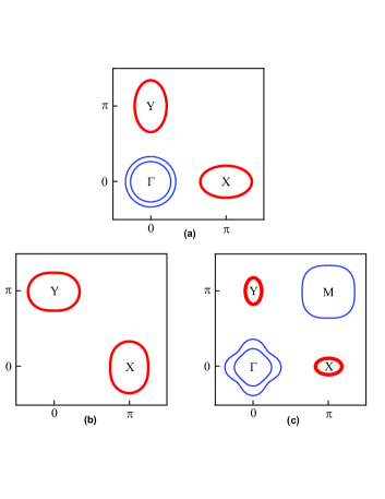
Figure 1: Schematic Fermi surfaces of three different systems where competing $s{}^{+-}$ and d-wave instabilities have been proposed CWu09 ; Fernandes13 ; Maiti12 ; s_plus_id_Khodas ; s_plus_id_Maier ; s_plus_id_Thomale . Thick/red (thin/blue) lines denote electron (hole) pockets. (a) In $\mathrm{Ba(Fe_{1-x}Mn_{x})_{2}As_{2}}$, the $s^{+-}$ state arise from $\left(\pi,0\right)/\left(0,\pi\right)$ stripe-type fluctuations, whereas the d-wave state comes from $\left(\pi,\pi\right)$ Neel-type fluctuations Fernandes13 . (b) In $A\mathrm{{}_{1-y}Fe_{2-x}Se_{2}}$ chalcogenides, a d-wave state appears due to the direct $XY$ interaction s_plus_id_Maier , whereas $s^{+-}$ is favored by FeAs hybridization s_plus_id_Khodas . (c) In strongly doped $\mathrm{(Ba_{1-x}K{}_{x})Fe_{2}As_{2}}$, the $s^{+-}$ state appears when small electron pockets emerge with doping, whereas a d-wave state can appear due to the $M$ intra-pocket interaction s_plus_id_Thomale ; Maiti12 .

While in most iron-based superconductors the pairing state is believed to be $s^{+-}$, both theoretical and experimental work suggests that a d-wave state may be nearby in free energy or even actually occur. In particular, in $\mathrm{(Ba_{1-x}K{}_{x})Fe_{2}As_{2}}$ and $\mathrm{Ba(Fe_{1-x}Mn_{x})_{2}As_{2}}$ pnictides and $A\mathrm{{}_{1-y}Fe_{2-x}Se_{2}}$ chalcogenides (see Fig. 1), calculations indicate that the a d-wave state may be tuned by varying the pnictogen height s_plus_id_Thomale , the $p-d$ orbital hybridization s_plus_id_Khodas , applied pressure Balatsky12 , and strength of Neel fluctuations Fernandes13 . Near the point where the $s$ and $d$ wave states cross in free energy, a time reversal symmetry breaking (TRSB) $s+id$ state has been predicted CWu09 ; Stanev10 . The experimental situation is not settled: in $\mathrm{(Ba_{1-x}K{}_{x})Fe_{2}As_{2}}$ the consensus is that at optimal doping $(x\approx 0.4)$ the state is fully gapped and of $s$ symmetry Shin_nodeless while in the $x=1$ compound thermal conductivity thermoconduct_KFe2As2 and ARPES measurements ARPES_KFe2As2 favor respectively a d-wave and a nodal $s^{+-}$ state. In $A\mathrm{{}_{1-y}Fe_{2-x}Se_{2}}$, inelastic neutron scattering Keimer_Fe2Se2 favors a d-wave state whereas ARPES indicates a nodeless s-wave state ARPES_Fe2Se2 . In the hole-doped $\mathrm{Ba(Fe_{1-x}Mn_{x})_{2}As_{2}}$, neutron scattering finds both Neel and stripe type magnetic fluctuations Mn_neutron – which favor d-wave and s-wave states, respectively – but no superconductivity has been observed. Raman scattering raman_mode in some of these materials indicate the existence of a Bardasis-Schrieffer mode, suggesting the presence of two competing SC instabilities. The unsettled experimental situation along with the compelling theoretical reasons to expect a proximal d-wave state motivates a more detailed examination of the physics associated with a change from $s$ to $d$-symmetry.

The change from $s^{+-}$ to d-wave superconductivity in the absence of nematicity CWu09 ; Stanev10 and the interplay between nematicity and a single SC order parameter Nandi10 ; Moon12 ; Fernandes_SUST have been studied. On general grounds, one expects that a single superconducting order parameter $\Delta$ couples to a nematic order parameter $\varphi$ via the biquadratic term $\Delta^{2}\varphi^{2}$ in the free energy Fernandes_arxiv13 . This coupling leads to a suppression of superconductivity in the presence of nematicity and vice-versa, as well as to a hardening of the shear modulus below $T_{c}$. These features have been reported in the $\mathrm{Ba(Fe_{1-x}Co_{x})_{2}As_{2}}$ materials Nandi10 ; shear_modulus .

The key new aspect of our analysis is that if both $s$ and $d$-symmetry superconductivity are important, then the free energy will contain also a tri-linear term

$$F_{\mathrm{SC-nem}}\propto\varphi\Delta_{s}\Delta_{d}\cos\theta$$ (1)

connecting the s-wave, d-wave, and nematic order parameters (here $\theta$ is the relative phase of the two SC order parameters). As we shall show this coupling implies that

• nematic order leads to an enhancement of the SC transition temperature;

• superconductivity can lead to the appearance of a nematic phase;

• an $s+d$ symmetry phase (similar to the one proposed in Ref. Livanas12 ) or a first-order transition can separate the pure $s^{+-}$ and d-wave states;

• a softening of the shear modulus below $T_{c}$ is an experimental signature of proximity to the regime where $s^{+-}$ and $d$-wave SC states are degenerate.

These results are robust and do not rely on any specific shape of the Fermi surface, as they follow from a general Ginzburg-Landau analysis based on a free energy that respects the gauge and rotational symmetries of the system:

$$F = F_{\mathrm{nem}}\left(\varphi^{2}\right)+\frac{t_{s}}{2}\Delta_{s}^{2}+\frac{t_{d}}{2}\Delta_{d}^{2}+\frac{\beta_{s}}{4}\Delta_{s}^{4}+\frac{\beta_{d}}{4}\Delta_{d}^{4}$$ (2)

$$+ \frac{1}{2}\Delta_{s}^{2}\Delta_{d}^{2}\left(\beta_{sd}+\alpha\cos 2\theta\right)+\lambda\varphi\Delta_{s}\Delta_{d}\cos\theta$$

Here $F_{\mathrm{nem}}$ is the free energy of the pure nematic phase, $t_{j}=a_{j}\left(T-T_{c,j}\right)$ with $a_{j}>0$ gives the distance to the SC transition temperatures in the $j=s^{+-},d$ channels, and $\lambda$, $\alpha$, and the $\beta_{i}$ are coupling constants. Note, the bi-quadratic couplings $\Delta_{s/d}^{2}\varphi^{2}$ are subleading near the s-d transition and are not written explicitly here. In the materials discussed above, $T_{c,s}$ and $T_{c,d}$ are tuned by the doping concentration $x$ due to different mechanisms: In $\mathrm{Ba(Fe_{1-x}Mn_{x})_{2}As_{2}}$ (Fig. 1a), increasing $x$ leads to stronger Neel fluctuations which favor the d-wave state Fernandes13 . In $A\mathrm{{}_{1-y}Fe_{2-x}Se_{2}}$ (Fig. 1b), changing $x$ modifies the Fe-As hybridization, which in turn favors either s-wave or d-wave s_plus_id_Khodas . In $\mathrm{(Ba_{1-x}K{}_{x})Fe_{2}As_{2}}$ (Fig. 1c), increasing $x$ gives rise to a large hole pocket at the $M$ point, which favors a d-wave state s_plus_id_Thomale ; Maiti12 . For illustration, in the Supplementary Material we derive this free energy from a BCS model appropriate for the system in Fig. 1a, but we emphasize that our conclusions are more general.

In the absence of significant nematicity, we find $\alpha>0$, implying that the free energy is minimized by setting $\theta=\pi/2$. We also find that $\left(\beta_{sd}-\left|\alpha\right|\right)^{2}<\beta_{s}\beta_{d}$, implying that the s-wave and d-wave states can be simultaneously present FernandesPRB10 . In this case, near the degeneracy point $T_{c,s}=T_{c,d}=T^{*}$, the two order parameters enter in the form $s+id$, breaking time-reversal symmetry. Note that microscopic models also found $s+id$ states in systems with the Fermi surfaces of Figs. 1b and 1c s_plus_id_Khodas ; s_plus_id_Thomale . The resulting phase diagram in the absence of nematicity is shown schematically in panel (a) of Fig. 2.

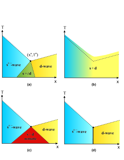
Figure 2: Schematic phase diagrams as function of temperature ($T$) and doping ($x$) for the interplay between $s^{+-}$-wave and d-wave superconductivity in iron pnictide materials. Dotted (solid) lines denote second (first) order phase transitions. Panel (a): no nematic order and weak nematic fluctuations ($\chi_{\mathrm{nem}}<2\alpha/\lambda^{2}$). The s-wave and d-wave states are separated by an intermediate time-reversal symmetry-breaking (TRSB) $s+id$ state. Panel (b): pre-existing nematic order. $T_{c}$ is enhanced with respect to the tetragonal case (dashed line), and the superconducting order parameter is characterized by the real combination $s+d$ and evolves smoothly with $x$ with no TRSB. Panel (c): no nematic order, but larger nematic fluctuations ($2\alpha<\lambda^{2}\chi_{\mathrm{nem}}<\beta_{sd}+\alpha+\sqrt{\beta_{s}\beta_{d}}$). The coexistence region is enhanced but the intermediate state is of $s+d$ character, spontaneously breaking rotational but not time reversal symmetry. Panel (d): no nematic order, but even larger nematic fluctuations ($\lambda^{2}\chi_{\mathrm{nem}}>\beta_{sd}+\alpha+\sqrt{\beta_{s}\beta_{d}}$). The s-wave to d-wave transition becomes first-order.

Including nematicity leads to significant changes. Consider first the case that a nematic phase transition occurs at a temperature far above the SC transition temperature. In this case, extremizing $F_{\mathrm{nem}}$ leads to a non-zero expectation value of the nematic order parameter $\left\langle\varphi\right\rangle=\varphi_{0}$ so the SC free energy contains an effective bilinear term $\lambda\varphi_{0}\Delta_{s}\Delta_{d}\cos\theta$. Diagonalizing the quadratic part of the free energy reveals that the energy minimum is at $\theta=0$ so the SC order parameter becomes a real admixture of $s$ and d-wave gaps, evolving smoothly across the degeneracy point (see Supplementary Material). $T_{c}$, determined from the solution of $t_{c}t_{d}=\lambda^{2}\varphi_{0}^{2}$, is enhanced relative to its tetragonal value $T_{c,s/d}$, with the enhancement being largest at the degeneracy point $T_{c,s}=T_{c,d}=T^{*}$ where we find the non-analytic behavior $T_{c}-T^{*}\propto\left|\varphi_{0}\right|$ and the maximal admixture between s-wave and d-wave states. Away from this point, $T_{c}-T_{c,s/d}\propto\varphi_{0}^{2}$. Figure 2(b) shows the phase diagram corresponding to this situation. We note that if the coupling $\lambda$ is not too strong, an $s+id$ phase may appear at lower temperatures s_plus_is .

We now consider that nematic order is absent but nematic fluctuations are important. In this case, we approximate $F_{\mathrm{nem}}=\frac{1}{2}\chi_{\mathrm{nem}}^{-1}\varphi^{2}$, where $\chi_{\mathrm{nem}}$ is the nematic susceptibility which would diverge at the nematic transition. Minimizing with respect to the nematic order parameter, we find $\varphi=-\lambda\chi_{\mathrm{nem}}\Delta_{s}\Delta_{d}\cos\theta$. Substituting back into Eq.  (2) yields:

$$\tilde{F} = \frac{t_{s}}{2}\Delta_{s}^{2}+\frac{t_{d}}{2}\Delta_{d}^{2}+\frac{\beta_{s}}{4}\Delta_{s}^{4}+\frac{\beta_{d}}{4}\Delta_{d}^{4}$$ (3)

$$+ \frac{1}{2}\Delta_{s}^{2}\Delta_{d}^{2}\left(\tilde{\beta}_{sd}+\tilde{\alpha}\cos 2\theta\right)$$

with $\tilde{\alpha}=\alpha-\frac{1}{2}\lambda^{2}\chi_{\mathrm{nem}}$ and $\tilde{\beta}_{sd}=\beta_{sd}-\frac{1}{2}\lambda^{2}\chi_{\mathrm{nem}}$. For weak nematic fluctuations, $\chi_{\mathrm{nem}}<2\alpha/\lambda^{2}$, $\tilde{\alpha}$ remains positive and the relative phase remains at $\theta=\pi/2$ so that the phase diagram retains the form displayed in Fig. 2(a), with $\varphi=0$.

As the nematic instability is approached, $\chi_{\mathrm{nem}}$ increases and eventually $\tilde{\alpha}$ changes sign so that the energy minimum shifts from $\theta=\pi/2$ to $\theta=0,\pi$. Note that the BCS calculations, which indicate that $\alpha<\beta_{sd}$, imply that the sign change in $\tilde{\alpha}$ happens before the condition for a second order phase transition is violated. Consequently, the SC state takes the real form $s\pm d$ and the nematic order parameter acquires a non-vanishing expectation value $\varphi=\pm\lambda\chi_{\mathrm{nem}}\Delta_{s}\Delta_{d}$ indicating a spontaneous breaking of tetragonal symmetry as shown in Fig. 2(c). Note that an $s\pm d$ state was also found in the $T=0$ numerical results of Ref. Livanas12 . As the nematic susceptibilty further increases, $\tilde{\beta}_{sd}$ changes sign and eventually the magnitude of $\left|\tilde{\beta}_{sd}-\tilde{\alpha}\right|$ becomes large enough that the transition between $s$ and $d$ becomes first order as shown in Fig. 2(d). An estimate for the critical nematic susceptibility above which $s\pm d$ emerges reveals that it corresponds to moderate fluctuations, which are reasonable to be expected in the real materials (see Supplementary Material). In this regard, note that shear modulus measurements have revealed the presence of significant nematic fluctuations in the phase diagrams of 122 compounds shear_modulus ; Yoshizawa12 .

The analysis so far has been based only on symmetry arguments, but it is of interest to demonstrate a mechanism and provide an estimate for the magnitude of the effect. We present a spin fluctuation Eliashberg calculation following Ref. Fernandes13 but including nematicity, for the system whose Fermi surface is displayed in Fig. 1(a), with hole pockets at the center of the Brillouin zone $\Gamma=\left(0,0\right)$ and electron pockets centered at $X=\left(\pi,0\right)$ and $Y=\left(0,\pi\right)$. Stripe spin fluctuations (peaked at $\mathbf{Q}_{X}=\left(\pi,0\right)$ and $\mathbf{Q}_{Y}=\left(0,\pi\right)$) induce repulsive $\Gamma-X$ and $\Gamma-Y$ interactions that favor an $s^{+-}$ state, whereas Neel fluctuations (peaked at $\mathbf{Q}_{N}=\left(\pi,\pi\right)$) induce a repulsive $X-Y$ interaction that favors a d-wave state Fernandes13 .

In the Eliashberg formalism, the pairing interactions are determined by the dynamic magnetic susceptibilities $\chi_{i}\left(\mathbf{Q}_{i}+\mathbf{q},\omega\right)$ with $i=X,Y,N$ (see Supplementary Material for more details). Neutron scattering experiments reveal that all of the relevant spin fluctuations are overdamped Mn_neutron , $\chi_{i}^{-1}\left(\mathbf{Q}_{i}+\mathbf{q},\omega\right)=\xi_{i}^{-2}+q^{2}-i\omega\gamma_{i}^{-1}$ and are characterized by two parameters: the magnetic correlation length $\xi_{i}$ and the Landau damping $\gamma_{i}$. As we have previously shown Fernandes13 , in the tetragonal phase where $\xi_{X}=\xi_{Y}=\xi_{S}$ the system undergoes a transition from an $s^{+-}$ to a d-wave SC state as the Neel correlation length $\xi_{N}$ increases from zero (see Fig. 3(a)).

In the presence of long-range nematic order, tetragonal symmetry is broken and the two stripe-type correlation lengths $\xi_{X}$ and $\xi_{Y}$ become different, with $\varphi=\ln\left(\xi_{X}/\xi_{Y}\right)$ Fernandes12 , implying that the pairing interaction is different between the $\Gamma-X$ and $\Gamma-Y$ pockets. In Fig. 3(a), we show the numerically calculated $T_{c}$ in the nematic phase. We observe a behavior similar to the schematic phase diagram of Fig. 2(b), with the maximum relative increase of $T_{c}$ at the s-wave/d-wave degeneracy point $\xi_{N}\approx 0.33\xi_{S}$. Far from this point, $T_{c}$ decreases as $\varphi^{2}$ for increasing nematic order, reflecting the usual competing bi-quadratic coupling $\varphi^{2}\Delta_{s}^{2}$ between orders that break different symmetries (Fig. 3b). As the degeneracy point is approached, the d-wave instability becomes closer in energy to the $s^{+-}$ one, and $T_{c}$ starts to increase with increasing nematic order as $\varphi^{2}$. In the vicinities of the degeneracy point, this behavior changes and we observe the increase of $T_{c}$ with $\left|\varphi\right|$ - a signature of the tri-linear coupling (1), as discussed within the Ginzburg-Landau model. From our numerical results, we can estimate the coupling constant $\lambda\approx 0.33$, i.e. making $\xi_{X}\approx 1.35\xi_{Y}$ leads to a $10\%$ enhancement of the relative transition temperature $\left(T_{c}-T_{c,0}\right)/T_{c,0}$.

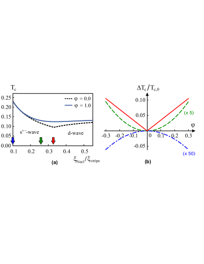
Figure 3: Dependence of $T_{c}$ on the Neel-type ($\xi_{\mathrm{Neel}}$) and stripe-type ($\xi_{\mathrm{stripe}}$) magnetic correlation lengths obtained from Eliashberg calculations as described in the text. Panel (a) shows the evolution of $T_{c}$ (in units of $\gamma_{\mathrm{stripe}}/2\pi$) as function of $\xi_{\mathrm{Neel}}/\xi_{\mathrm{stripe}}$ in the absence (dashed line) and presence of nematic order (solid line, $\varphi=1.0$). Panel (b) presents the variation of $T_{c}$, $\Delta T_{c}=T_{c}-T_{c,0}$, as function of the nematic order parameter $\varphi=\ln\left(\xi_{X}/\xi_{Y}\right)$, for three fixed values of the ratio $\xi_{\mathrm{Neel}}/\xi_{\mathrm{stripe}}$ indicated by the arrows in panel (a): $\xi_{\mathrm{Neel}}/\xi_{\mathrm{stripe}}=0.1$ (dotted-dashed, blue online), $\xi_{\mathrm{Neel}}/\xi_{\mathrm{stripe}}=0.26$ (dashed, green online), and $\xi_{\mathrm{Neel}}/\xi_{\mathrm{stripe}}=0.33$ (solid, red online).

Measurements of elastic anomalies across the superconducting transition can also reveal the strength of the tri-linear coupling. The idea, which goes back to the work of Testardi and others on the A-15 materials Testardi and was revisited in the context of the cuprates Millis_Rabe , is that within mean field theory, as the temperature is decreased below $T_{c}$, the free energy acquires an additional contribution

$$\Delta F=-\frac{1}{2}\frac{\Delta C}{T_{c}}\left(T-T_{c}(\varphi)\right)^{2}$$ (4)

Here $\Delta C$ is the specific heat jump across the transition. The crucial point is that the dependence of $T_{c}$ on the strain (proportional to $\varphi$) leads to new contributions to the elastic free energy which are singular at $T_{c}$ and proportional to the strain derivatives of $T_{c}$ and to $\Delta C$. Differentiating Eq. 4 twice with respect to strain and retaining only the most singular terms at $T_{c}$ gives discontinuities in the shear elastic modulus $C_{66}$ and its first temperature derivative

$$\Delta C_{66}\equiv C_{66}(T_{c}^{-})-C_{66}(T_{c}^{+}) = -\frac{\Delta C}{T_{c}}\left(\frac{\partial T_{c}}{\partial\varphi}\right)^{2}$$ (5)

$$\Delta\frac{dC_{66}}{dT} = \frac{\Delta C}{T_{c}}\frac{\partial^{2}T_{c}}{\partial\varphi^{2}}$$ (6)

In the nematic phase or at the $s-d$ degeneracy point in Fig. 2(c), because $T_{c}$ depends linearly on $\varphi$, the elastic modulus exhibits a downwards jump (softening) across $T_{c}$. In the tetragonal phase, $T_{c}$ depends quadratically on $\varphi$. Far from the $s-d$ degeneracy point, the $\varphi^{2}\Delta^{2}$ free energy term discussed in Nandi10 ; Fernandes_arxiv13 - present in the Eliashberg calculations but not explicitly written in Eq. (2) - gives a negative $\partial^{2}T_{c}/\partial\varphi^{2}$ (see Fig. 3b). This implies a hardening of $C_{66}$ below $T_{c}$, as observed in optimally doped $\mathrm{Ba(Fe_{1-x}Co_{x})_{2}As_{2}}$ shear_modulus ; Yoshizawa12 . However, as the d-wave state is approached, the tri-linear coupling leads to a positive contribution $\lambda^{2}/t_{d}$ to $\partial^{2}T_{c}/\partial\varphi^{2}$ which diverges at the degeneracy point, causing a softening in $C_{66}$. A softening of $C_{66}$ across $T_{c}$ is thus a clear signal of proximity between s-wave and d-wave states.

Compounds to which the considerations of this paper may be relevant include $A\mathrm{{}_{1-y}Fe_{2-x}Se_{2}}$ chalcogenides, where neutron scattering Keimer_Fe2Se2 and ARPES ARPES_Fe2Se2 seem to support different pairing states, and $\mathrm{KFe_{2}As_{2}}$, where experiment suggests a change in pairing state with applied pressure Taillefer_pressure . Further, in the optimally doped compound $\mathrm{BaFe_{2}(As_{1-x}P_{x})_{2}}$, recent detwinning experiments found an unexpected enhancement of $T_{c}$ with the applied strain Kuo12 , as expected if the tri-linear coupling is relevant.

The results here may also help to resolve a controversy concerning the superconducting state of the extremely overdoped pnictide compound $\mathrm{(Ba_{1-x}K{}_{x})Fe_{2}As_{2}}$, which is believed to possess the Fermi surface shown in Fig. 1(c). ARPES experiments ARPES_KFe2As2 support a scenario where the SC state evolves from nodeless $s^{+-}$ at optimal doping $x_{\mathrm{opt}}\approx 0.4$ towards nodal $s^{+-}$ at $x=1$ (with a possible intermediate TRSB $s+is$ state s_plus_is ). Thermal conductivity measurements thermoconduct_KFe2As2 support a transition from nodeless $s^{+-}$ at $x_{\mathrm{opt}}$ to d-wave at $x=1$. Calculations Thomale11 ; Maiti12 indicate that the two states have comparable transition temperatures. The results of this paper indicate that if the second state is d-wave then a structural/nematic “dome”, detectable by x-ray Nandi10 or torque magnetometry Matsuda12 , could appear in the vicinity of the critical $x$. Also, application of a stress field to induce long-range nematic order Fisher12 would cause a linear increase in $T_{c}$. A softening of the elastic modulus across the transition would further support a d-wave state.

In summary, our results unveil a unique feature of the interplay between nematicity and SC in iron-based materials. The tri-linear coupling (1) shows that at the same time that the d-wave and s-wave gaps work together as an effective field conjugate to the nematic order parameter, allowing for spontaneous tetragonal symmetry breaking in the superconducting state, nematicity leads to an effective attraction between the two otherwise competing states. This physics can also be expected in other situations where multiple SC instabilities are present, such as the ruthenates $\mathrm{Sr_{2}RuO_{4}}$, where a chiral triplet $p+ip$ state has been proposed, and the consequences for the elastic modulus discontinuties of tri-linear coupling $\varphi p_{x}p_{y}$ have been discussed Sigrist ; Walker02 .

Acknowledgments We thank A. Chubukov, E. Fradkin, S. Maiti, C. Meingast, J. Schmalian, and L. Taillefer for inspiring discussions. AJM was supported by NSF DMR 1006282.

Supplementary material for “Nematicity as a probe of superconducting pairing in iron-based superconductors"

I Microscopic derivation of the free energy

We consider the Fermi surface displayed in Fig. 1a of the main text, with hole pockets at the center of the Brillouin zone $\Gamma=\left(0,0\right)$ and electron pockets centered at $X=\left(\pi,0\right)$ and $Y=\left(0,\pi\right)$. For simplicity, we assume the two hole pockets to be degenerate and label the pockets by $i=\Gamma,X,Y$. Stripe-type spin fluctuations induce repulsive hole pocket-electron pocket interactions $\bar{U}_{\Gamma X}$ and $\bar{U}_{\Gamma Y}$, whereas Neel-type fluctuations give rise to a repulsive electron pocket-electron pocket interaction $\bar{U}_{XY}$. The free energy density $F$ is given by FernandesPRB10 ; s_plus_is :

$$F=\sum_{i,j}\Delta_{i}U_{ij}^{-1}\Delta_{j}^{*}-\sum_{i}\frac{1}{N_{i}}\left(\int_{k}G_{i,k}G_{i,-k}\right)\left|\Delta_{i}\right|^{2}+\sum_{i}\frac{1}{2N_{i}^{2}}\left(\int_{k}G_{i,k}^{2}G_{i,-k}^{2}\right)\left|\Delta_{i}\right|^{4}$$ (S1)

where $i=\Gamma,X,Y$ is the band index, $G_{i,k}^{-1}=i\omega_{n}-\varepsilon_{i,\mathbf{k}}$ is the bare Green’s function of band $i$, $k=\left(\omega_{n},\mathbf{k}\right)$ labels the momentum $\mathbf{k}$ and the fermionic Matsubara frequency $\omega_{n}=(2n+1)\pi T$, $\int_{k}=T\sum_{\omega_{n}}\int\frac{d^{d}k}{\left(2\pi\right)^{d}}$. The gap functions have been rescaled from the standard BCS definitions as $\Delta_{i}=\Delta_{i,0}\sqrt{N_{i}}$ where $N_{i}$ is the density of states of band $i$ and $U_{ij}$ are the components of the interaction matrix

$$\mathbf{U}=\left(\begin{array}[]{ccc}0&-\lambda_{X\Gamma}&-\lambda_{Y\Gamma}\\ -\lambda_{X\Gamma}&0&-\lambda_{XY}\\ -\lambda_{Y\Gamma}&-\lambda_{XY}&0\end{array}\right)$$ (S2)

where $\lambda_{ij}=\bar{U}_{ij}\sqrt{N_{i}N_{j}}$. In the tetragonal phase, $\lambda_{X\Gamma}=\lambda_{Y\Gamma}$; nematic order leads to a difference between the two coefficients and also makes $N_{X}\neq N_{Y}$.

Evaluation of the Green’s function products yields

$$F=\sum_{i,j}\Delta_{i}U_{ij}^{-1}\Delta_{j}^{*}-\ln\left(\frac{W}{T}\right)\sum_{i}\left|\Delta_{i}\right|^{2}+\sum_{i}\frac{u_{0}}{N_{i}}\left|\Delta_{i}\right|^{4}$$ (S3)

with $u_{0}=\frac{7\zeta\left(3\right)}{16\pi^{2}T^{2}}>0$ and $W$ a cutoff set by the smaller of the frequency cutoff of the interaction and the distance from the Fermi level to the band edge.

We begin our analysis of Eq. S3 by diagonalizing the quadratic term. In the tetragonal symmetry case, where $\lambda_{X\Gamma}=\lambda_{Y\Gamma}$, the three eigenvalues and corresponding eigenvectors of the $U$ matrix are (we define the basis as $\left(\Gamma,X,Y\right)$)

$$\Delta_{s^{++}} = \left(\begin{array}[]{c}\sin\Psi\\ \frac{1}{\sqrt{2}}\cos\Psi\\ \frac{1}{\sqrt{2}}\cos\Psi\end{array}\right);\leavevmode\nobreak\ \leavevmode\nobreak\ \lambda_{s^{++}}=-\sqrt{2}\lambda_{X\Gamma}\cot\Psi$$ (S7)

$$\Delta_{s^{+-}} = \left(\begin{array}[]{c}-\cos\Psi\\ \frac{1}{\sqrt{2}}\sin\Psi\\ \frac{1}{\sqrt{2}}\sin\Psi\end{array}\right);\leavevmode\nobreak\ \leavevmode\nobreak\ \lambda_{s^{+-}}=\sqrt{2}\lambda_{X\Gamma}\tan\Psi$$ (S11)

$$\Delta_{d} = \left(\begin{array}[]{c}0\\ -\frac{1}{\sqrt{2}}\\ \frac{1}{\sqrt{2}}\end{array}\right);\leavevmode\nobreak\ \leavevmode\nobreak\ \lambda_{d}=\lambda_{XY}$$ (S15)

with

$$\tan\Psi=\frac{\sqrt{8\lambda_{X\Gamma}^{2}+\lambda_{XY}^{2}}-\lambda_{XY}}{2\sqrt{2}\lambda_{X\Gamma}}$$ (S16)

The three solutions correspond, respectively, to the $s_{++}$ state (gap functions of equal sign in all the Fermi pockets), to the $s_{++}$ state (equal sign in the electron pockets, opposite sign in the hole pocket), and to the d-wave state (opposite signs in the electron pockets).

Inverting the equations to obtain expressions for the order parameter in the band basis yields:

$$\Delta_{\Gamma} = -\cos\Psi\Delta_{s^{+-}}+\sin\Psi\Delta_{s^{++}}$$

$$\Delta_{X} = \frac{1}{\sqrt{2}}\left(-\Delta_{d}+\sin\Psi\Delta_{s^{+-}}+\cos\Psi\Delta_{s^{++}}\right)$$

$$\Delta_{Y} = \frac{1}{\sqrt{2}}\left(\Delta_{d}+\sin\Psi\Delta_{s^{+-}}+\cos\Psi\Delta_{s^{++}}\right)$$ (S17)

which can be equivalently written in terms of the vectors $\boldsymbol{\Delta}_{\mathrm{band}}=\left(\begin{array}[]{ccc}\Delta_{\Gamma}&\Delta_{X}&\Delta_{Y}\end{array}\right)^{T}$, $\boldsymbol{\Delta}_{\mathrm{sym}}=\left(\begin{array}[]{ccc}\Delta_{s^{++}}&\Delta_{s^{+-}}&\Delta_{d}\end{array}\right)^{T}$, and transformation matrix:

$$\boldsymbol{\Lambda}=\left(\begin{array}[]{ccc}\sin\Psi&-\cos\Psi&0\\ \frac{\cos\Psi}{\sqrt{2}}&\frac{\sin\Psi}{\sqrt{2}}&-\frac{1}{\sqrt{2}}\\ \frac{\cos\Psi}{\sqrt{2}}&\frac{\sin\Psi}{\sqrt{2}}&+\frac{1}{\sqrt{2}}\end{array}\right)$$ (S18)

as:

$$\boldsymbol{\Delta}_{\mathrm{band}}=\boldsymbol{\Lambda}\boldsymbol{\Delta}_{\mathrm{sym}}$$ (S19)

Substituting this into the first two terms of Eq. S3, we obtain the quadratic term $F^{(2)}$:

$$F^{(2)}=\frac{t_{s^{++}}}{2}\left|\Delta_{s^{+-}}\right|^{2}+\frac{t_{s^{+-}}}{2}\left|\Delta_{s^{+-}}\right|^{2}+\frac{t_{d}}{2}\left|\Delta_{d}\right|^{2}$$ (S20)

with

$$t_{i}=\frac{1}{\lambda_{i}}-\ln\left(\frac{W}{T}\right)$$ (S21)

Therefore, the transition temperature is given by $T_{c}=W\exp\left(-1/\lambda_{\mathrm{max}}\right)$, where $\lambda_{\mathrm{max}}$ is the largest of the eigenvalues of the $U_{ij}$ interaction matrix. Since $\lambda_{s^{++}}<0$ always, the $s^{++}$ state is never realized, so we set $\Delta_{s^{++}}=0$ hereafter. Analyzing the eigenvalues, we find that, for $\lambda_{XY}<\lambda_{X\Gamma}$, the leading instability is towards an $s^{+-}$ state, whereas for $\lambda_{XY}>\lambda_{X\Gamma}$, it is towards a d-wave state. The phase diagram is shown in Fig. S1. Note that the $s^{+-}$/d-wave degeneracy point $\lambda_{XY}=\lambda_{X\Gamma}$ corresponds to $\tan\Psi=1/\sqrt{2}$, what implies $\cos\Psi=\sqrt{2/3}$ and $\sin\Psi=1/\sqrt{3}$.

To obtain the quartic term $F^{(4)}$ of the free energy, we substitute (S17) in the last term of the free energy (S3), obtaining:

$$\frac{F^{(4)}}{u_{0}}=\left(\frac{\cos^{4}\Psi}{N_{\Gamma}}+\frac{\sin^{4}\Psi}{2N_{X}}\right)\left|\Delta_{s^{+-}}\right|^{4}+\frac{1}{2N_{X}}\left|\Delta_{d}\right|^{4}+\frac{2\sin^{2}\Psi}{N_{X}}\left|\Delta_{s^{+-}}\right|^{2}\left|\Delta_{d}\right|^{2}\left(1+\frac{1}{2}\cos 2\theta\right)$$ (S22)

which can also be expressed in the form:

$$F^{(4)}=\frac{\beta_{s}}{4}\left|\Delta_{s^{+-}}\right|^{4}+\frac{\beta_{d}}{4}\left|\Delta_{d}\right|^{4}+\frac{1}{2}\left|\Delta_{s^{+-}}\right|^{2}\left|\Delta_{d}\right|^{d}\left(\beta_{sd}+\alpha\cos 2\theta\right)$$ (S23)

with the Ginzburg-Landau coefficients $\beta_{d}=2u_{0}/N_{X}$ and:

$$\beta_{s} = \beta_{d}\left(\frac{2N_{X}}{N_{\Gamma}}\cos^{4}\Psi+\sin^{4}\Psi\right)$$ (S24)

$$\beta_{sd} = 2\beta_{d}\sin^{2}\Psi$$ (S25)

$$\alpha = \frac{\beta_{sd}}{2}$$ (S26)

Here, $\theta$ is the relative phase between the d-wave and $s^{+-}$ gaps. Note that we have $\alpha>0$ and:

$$\frac{\left(\beta_{sd}-\alpha\right)^{2}}{\beta_{s}\beta_{d}}=\left(1+\frac{2N_{X}}{N_{\Gamma}}\cot^{4}\Psi\right)^{-1}<1$$

implying that there is an $s+id$ coexistence state below the $s^{+-}$/d-wave degeneracy point in the tetragonal-symmetric case. The expressions given in the main text are obtained by evaluating the equations above at the degeneracy point, where $\tan\Psi=1/\sqrt{2}$, and also assuming $N_{X}\approx N_{\Gamma}$.

The formulae given above are derived assuming tetragonal symmetry. In the nematic phase, the leading order effect of a tetragonal symmetry breaking is a change in the interaction matrix $\mathbf{U}\rightarrow{\mathbf{U}+\delta\mathbf{U}}$ with (in the $\Gamma,X,Y$ basis)

$$\delta\mathbf{U}=\frac{\zeta}{2}\left(\begin{array}[]{ccc}0&-\varphi&\varphi\\ -\varphi&0&0\\ \varphi&0&0\end{array}\right)$$ (S27)

where $\varphi$ is the nematic order parameter and $\zeta$ is a coupling constant describing how the interactions $\lambda_{ij}$ change in the presence of nematic order, i.e. $\lambda_{\left(X,Y\right)\Gamma}\rightarrow\lambda_{\left(X,Y\right)\Gamma}\pm\zeta\varphi$. Numerically, it is straightforward to obtain $T_{c}$ for a finite $\varphi$ by directly diagonalizing $\mathbf{U}+\delta\mathbf{U}$. The results, presented in figure S1, show that $T_{c}$ increases for a finite nematic order parameter, with a pronounced peak at the degeneracy point $\lambda_{X\Gamma}=\lambda_{Y\Gamma}$. Figure S1 shows that in the entire phase diagram, the eigenvector corresponding to the leading eigenvalue has contributions coming from all three components $s_{++}$, $s_{+-}$, and d-wave, with the latter being responsible for the main contributions.

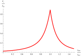
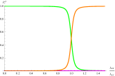
Figure S1: (upper left panel) $T_{c}$ (in units of the cutoff $W$) as function of the d-wave pairing interaction $\lambda_{XY}$ (in units of the s-wave interaction $\lambda_{X\Gamma}=0.2$) for $\varphi=0$ (blue curve) and $\varphi=0.05/\zeta$ (red curve). (upper right panel) Ratio between $T_{c}$ for $\varphi=0.05/\zeta$ and $T_{c,0}$ in the tetragonal phase ($\varphi=0$) as function of the d-wave pairing interaction $\lambda_{XY}$ (in units of the s-wave interaction $\lambda_{X\Gamma}=0.2$). (lower panel). As function of the d-wave pairing interaction $\lambda_{XY}$, we present the projection $P_{i}=\left\langle\Delta_{\varphi}\left.\right|\Delta_{i}\right\rangle$ of the eigenvector $\Delta_{\varphi}$ that diagonalizes the problem in the nematic phase ($\varphi=0.01/\zeta$) along the three eigenvectors $\Delta_{i}$ of the tetragonal phase: $s_{++}$ (magenta), $s_{+-}$ (green curve), and d-wave (orange).

To understand this increase in $T_{c}$, we use the transformation matrix $\boldsymbol{\Lambda}$ in Eq. (S18) to project the gap equation $\left(\mathbf{U+\delta U}\right)\ln\frac{W}{T_{c}}=\mathbf{1}$ onto the $s^{+-}$ and $d$ subspace, yielding:

$$1=\ln\frac{W}{T_{c}}\left(\begin{array}[]{cc}\lambda_{s^{+-}}&-\frac{\zeta\cos\Psi}{\sqrt{2}}\,\varphi\\ -\frac{\zeta\cos\Psi}{\sqrt{2}}\,\varphi&\lambda_{d}\end{array}\right)$$ (S28)

Diagonalizing this matrix, we find $T_{c}=W\exp\left(-1/\lambda_{\mathrm{max}}\right)$ with the leading eigenvalue

$$\lambda_{\mathrm{max}}=\left(\frac{\lambda_{s^{+-}}+\lambda_{d}}{2}\right)+\sqrt{\left(\frac{\lambda_{s^{+-}}-\lambda_{d}}{2}\right)^{2}+\frac{\zeta^{2}\cos^{2}\Psi}{2}\,\varphi^{2}}$$ (S29)

which is clearly greater than either $\lambda_{s^{+-}}$ or $\lambda_{d}$ if $\varphi\neq 0$, so that $T_{c}$ is increased in the nematic phase. In particular, at the degeneracy point $\lambda_{s^{+-}}=\lambda_{d}$ the increase is linear in $\left|\varphi\right|$; away from this point, the variation with $\varphi$ is quadratic. Note that the eigenvector is a real admixture of $s^{+-}$ and d-wave contributions, with equal weights at the degeneracy point.

To obtain the coupling between the nematic and the SC order parameters, we take the inverse $\left(\mathbf{U}+\delta\mathbf{U}\right)^{-1}\approx\mathbf{U}^{-1}-\mathbf{U}^{-1}\delta\mathbf{U}\,\mathbf{U}^{-1}$ to leading order in $\zeta$, substitute in the first term of Eq. (S3), and change basis via $\boldsymbol{\Lambda}$, yielding:

$$F\left(\varphi\right)=F\left(\varphi=0\right)-\boldsymbol{\Delta}\left(\boldsymbol{\Lambda}^{T}\mathbf{U}^{-1}\boldsymbol{\Lambda}\right)\left(\boldsymbol{\Lambda}^{T}\delta\mathbf{U}\>\boldsymbol{\Lambda}\right)\left(\boldsymbol{\Lambda}^{T}\mathbf{U}^{-1}\boldsymbol{\Lambda}\right)\boldsymbol{\Delta}^{*}$$ (S30)

Evaluation of the matrix products then yields the tri-linear term:

$$F\left(\varphi\right)=F\left(\varphi=0\right)+\left(\frac{\zeta\cos^{2}\Psi}{\lambda_{X\Gamma}\lambda_{XY}\sin\Psi}\right)\varphi\left|\Delta_{s^{+-}}\right|\left|\Delta_{d}\right|\cos\theta$$ (S31)

The tri-linear coupling constant reduces to $\lambda=2\zeta/\left(\sqrt{3}\lambda_{X\Gamma}^{2}\right)$ at the degeneracy point.

II Eliashberg equations for the interplay between $s^{+-}$, $d$-wave, and nematicity

We now generalize the weak-coupling BCS model of the previous section to an Eliashberg calculation that takes into account the explicit form of the dynamic spin fluctuation susceptibilities $\chi_{i}\left(\mathbf{Q}_{i}+\mathbf{q},\omega\right)$, where $\mathbf{Q}_{i}$ refers to either the magnetic stripe-state ordering vectors $\mathbf{Q}_{1}=\left(\pi,0\right)$ and $\mathbf{Q}_{2}=\left(0,\pi\right)$ or the Neel ordering vector $\mathbf{Q}_{3}=\left(\pi,\pi\right)$. In each channel, we have overdamped spin dynamics:

$$\chi_{i}\left(\mathbf{q}+\mathbf{Q}_{i},\Omega_{n}\right)=\frac{1}{\left|\Omega_{n}\right|\gamma_{i}^{-1}+q^{2}+\xi_{i}^{-2}}$$

where $\gamma_{i}$ is the Landau damping and $\xi_{i}$ is the magnetic correlation length (measured in units of the lattice parameter). When coupled to the electronic degrees of freedom, via coupling constants $g_{i}$, these magnetic fluctuations give rise to the repulsive electronic interactions responsible for $s^{+-}$ and $d$-wave pairing.

This model is a generalization of the 3-band Eliashberg formalism introduced by us in Ref. Fernandes13 . Following that notation, we define the effective SC coupling constants:

$$\lambda_{1} \equiv 2g_{1}^{2}\sqrt{N_{\Gamma}N_{X}}$$

$$\lambda_{3} \equiv g_{3}^{2}N_{x}$$ (S32)

and the ratio between the density of states $r\equiv N_{X}/N_{\Gamma}$. Then, the Eliashberg equations are given by:

$$\frac{Z_{\Gamma,n}\omega_{n}}{T} = \left(2n+1\right)+\frac{\lambda_{1}\sqrt{r}}{2}\sum_{m}\mathrm{sgn}\left(2m+1\right)\left(\xi_{1}a_{nm}^{(1)}+\xi_{2}a_{nm}^{(2)}\right)$$

$$\frac{Z_{X,n}\omega_{n}}{T} = \left(2n+1\right)+\sum_{m}\mathrm{sgn}\left(2m+1\right)\left(\frac{\lambda_{1}\xi_{1}}{\sqrt{r}}a_{nm}^{(1)}+\lambda_{3}\xi_{3}a_{nm}^{(3)}\right)$$

$$\frac{Z_{Y,n}\omega_{n}}{T} = \left(2n+1\right)+\sum_{m}\mathrm{sgn}\left(2m+1\right)\left(\frac{\lambda_{1}\xi_{2}}{\sqrt{r}}a_{nm}^{(2)}+\lambda_{3}\xi_{3}a_{nm}^{(3)}\right)$$ (S33)

as well as:

$$W^{\prime}_{\Gamma,n} = -\frac{\lambda_{1}}{2}T\sum_{m}\left[\frac{W^{\prime}_{X,m}}{Z_{X,m}\left|\omega_{m}\right|}\,\xi_{1}a_{nm}^{(1)}+\frac{W^{\prime}_{Y,m}}{Z_{Y,m}\left|\omega_{m}\right|}\,\xi_{2}a_{nm}^{(2)}\right]$$

$$W^{\prime}_{X,n} = -\lambda_{1}\xi_{1}T\sum_{m}\frac{W^{\prime}_{\Gamma,m}}{Z_{\Gamma,m}\left|\omega_{m}\right|}\,a_{nm}^{(1)}-\lambda_{3}\xi_{3}T\sum_{m}\frac{W^{\prime}_{Y,m}}{Z_{Y,m}\left|\omega_{m}\right|}\,a_{nm}^{(3)}$$

$$W^{\prime}_{Y,n} = -\lambda_{1}\xi_{2}T\sum_{m}\frac{W^{\prime}_{\Gamma,m}}{Z_{\Gamma,m}\left|\omega_{m}\right|}\,a_{nm}^{(2)}-\lambda_{3}\xi_{3}T\sum_{m}\frac{W^{\prime}_{X,m}}{Z_{X,m}\left|\omega_{m}\right|}\,a_{nm}^{(3)}$$ (S34)

where $Z_{i,n}$ and $W_{i}$ are the frequency-dependent normal and anomalous components of the self-energy, associated with the mass renormalization and the gap functions, respectively. These quantities correspond to averages around each Fermi pocket - note that the orbital content of the Fermi surface is incorporated in the coupling constants, as explained in Ref. Fernandes13 . Finally, notice that we rescaled the $W_{i}$ functions as $W{}_{X,Y}=W^{\prime}_{X,Y}\sqrt{N_{\Gamma}}$ and $W{}_{\Gamma}=W^{\prime}_{\Gamma}\sqrt{N_{X}}$. The Matsubara-axis interactions $a_{nm}^{(i)}$, generated by the spin fluctuation spectra, are given by:

$$a_{nm}^{(i)}=\frac{1}{\sqrt{1+\left|n-m\right|2\pi T\gamma_{i}^{-1}\xi_{i}^{2}}}$$ (S35)

The sums in the $Z$ functions can be evaluated analytically. By introducing the auxiliary function:

$$S_{i,n}=\frac{2\,\mathrm{sgn}\left(n\right)}{\sqrt{2\pi T\gamma_{i}^{-1}\xi_{i}^{2}}}\left[\mathrm{Hw}\left(\frac{1}{2},1+\frac{1}{2\pi T\gamma_{i}^{-1}\xi_{i}^{2}}\right)-\mathrm{Hw}\left(\frac{1}{2},\left|n\right|+\frac{\mathrm{sgn}\left(n\right)+1}{2}+\frac{1}{2\pi T\gamma_{i}^{-1}\xi_{i}^{2}}\right)\right]+\mathrm{sgn}\left(n\right)$$ (S36)

for $n\neq 0,-1$ and $S_{i,n}=2\,\mathrm{sgn}\left(n\right)+1$ for $n=0,-1$, where $\mathrm{Hw}(x)$ is the Huruwitz zeta function, we obtain:

$$\frac{Z_{\Gamma,n}\omega_{n}}{T} = \left(2n+1\right)+\frac{\sqrt{r}\lambda_{1}\xi_{1}}{2}S_{1,n}+\frac{\sqrt{r}\lambda_{1}\xi_{2}}{2}S_{2,n}$$

$$\frac{Z_{X,n}\omega_{n}}{T} = \left(2n+1\right)+\frac{\lambda_{1}\xi_{1}}{\sqrt{r}}S_{1,n}+\lambda_{3}\xi_{3}S_{3,n}$$

$$\frac{Z_{Y,n}\omega_{n}}{T} = \left(2n+1\right)+\frac{\lambda_{1}\xi_{2}}{\sqrt{r}}S_{2,n}+\lambda_{3}\xi_{3}S_{3,n}$$ (S37)

For the gap functions, we introduce $\bar{\Delta}_{i,n}\equiv\frac{W^{\prime}_{i,n}}{Z_{i,n}\left|\omega_{n}\right|}$, yielding:

$$\bar{\Delta}_{\Gamma,n}\frac{Z_{\Gamma,n}\left|\omega_{n}\right|}{T} = -\frac{\lambda_{1}}{2}\,\xi_{1}\sum_{m}\bar{\Delta}_{X,m}a_{nm}^{(1)}-\frac{\lambda_{1}}{2}\,\xi_{2}\sum_{m}\bar{\Delta}_{Y,m}a_{nm}^{(2)}$$

$$\bar{\Delta}_{X,n}\frac{Z_{X,n}\left|\omega_{n}\right|}{T} = -\lambda_{1}\xi_{1}\sum_{m}\bar{\Delta}_{\Gamma,m}a_{nm}^{(1)}-\lambda_{3}\xi_{3}\sum_{m}\bar{\Delta}_{Y,m}a_{nm}^{(3)}$$

$$\bar{\Delta}_{Y,n}\frac{Z_{Y,n}\left|\omega_{n}\right|}{T} = -\lambda_{1}\xi_{2}\sum_{m}\bar{\Delta}_{\Gamma,m}a_{nm}^{(2)}-\lambda_{3}\xi_{3}\sum_{m}\bar{\Delta}_{X,m}a_{nm}^{(3)}$$ (S38)

Thus, we can write the gap equations in matrix form as:

$$\sum_{m,\nu}\tilde{K}_{mn}^{\mu\nu}\tilde{\Delta}_{m}^{\nu}=0$$ (S39)

where $\mu,\nu=1,2,3$ and the matrices are given by:

$$\left(\tilde{\Delta}_{m}\right)\equiv\left(\begin{array}[]{c}\bar{\Delta}_{\Gamma,m}\\ \bar{\Delta}_{X,m}\\ \bar{\Delta}_{Y,m}\end{array}\right)$$ (S40)

and:

$$\left(\tilde{K}_{nm}\right)\equiv\left(\begin{array}[]{ccc}-\delta_{nm}\frac{Z_{\Gamma,n}\left|\omega_{n}\right|}{T}&-\frac{1}{2}\,\lambda_{1}\xi_{1}a_{nm}^{(1)}&-\frac{1}{2}\,\lambda_{1}\xi_{2}a_{nm}^{(2)}\\ -\lambda_{1}\xi_{1}a_{nm}^{(1)}&-\delta_{nm}\frac{Z_{X,n}\left|\omega_{n}\right|}{T}&-\lambda_{3}\xi_{3}a_{nm}^{(3)}\\ -\lambda_{1}\xi_{2}a_{nm}^{(2)}&-\lambda_{3}\xi_{3}a_{nm}^{(3)}&-\delta_{nm}\frac{Z_{Y,n}\left|\omega_{n}\right|}{T}\end{array}\right)$$ (S41)

The transition temperature is found when the largest eigenvalue of the $\tilde{K}$ matrix vanishes. Following Ref. Fernandes13 , we used the parameters $\lambda_{1}=0.4$, $\lambda_{2}=0.8$, $r=0.65$, $\gamma_{3}/\gamma_{1}=0.33$, $\gamma_{1}=25$meV, and $\xi_{0}=5$. All temperatures are given in units of $\gamma_{1}/2\pi$. In the tetragonal phase, we have $\xi_{1}=\xi_{2}=\xi_{0}$, and changing the Neel correlation length $\xi_{3}$ induces an $s^{+-}$ to d-wave transition, as shown in Fig. 3a of the main text.

In the nematic phase, long-range nematic order changes the magnetic spectrum, making the $\left(\pi,0\right)$ and $\left(0,\pi\right)$ correlation lengths unequal, $\xi_{1}\neq\xi_{2}$. To perform our calculations in the nematic phase, displayed in Fig. 3 of the main text, we used the model of Ref. Fernandes12 to relate the nematic order parameter $\varphi$ to the changes in the correlation lengths for a quasi-2D system, $\xi_{1,2}=\xi_{0}/\sqrt{\varphi\left(\coth\varphi\mp 1\right)}$, implying $\varphi=\ln\left(\xi_{1}/\xi_{2}\right)$.

III Estimate for the critical nematic susceptibility

In the main text, we derived the critical nematic susceptibility $\chi_{\mathrm{nem}}^{c}$ above which the system displays an $s\pm d$ state and spontaneously breaks tetragonal symmetry, $\chi_{\mathrm{nem}}^{c}\equiv 2\alpha\lambda^{-2}$. Using the results of the previous sections, we can estimate this critical value. We have $\alpha=\frac{2}{3N_{X}}\left(\frac{7\zeta\left(3\right)}{16\pi^{2}T_{c}^{2}}\right)$ and $\lambda\approx 0.33$, according to the numerical calculations presented in Fig. 3 of the main text. The density of states can be estimated as $N_{X}\approx\varepsilon_{0}^{-1}$ where $\varepsilon_{0}\approx 100$ meV is the Fermi energy of the Fermi pockets. Using $T_{c}\approx\Delta\approx 3$ meV, we obtain $\chi_{\mathrm{nem}}^{c}\approx 7$ meV^-1. To have an idea of how strong this susceptibility is, we can estimate the magnitude of the shear modulus softening caused by it. Using the expression of Ref. shear_modulus , the relative reduction in the high-temperature shear modulus $C_{s,0}$ is given by $\left(\frac{C_{s}}{C_{s,0}}\right)=\left(1+\frac{\lambda_{\mathrm{el}}^{2}\chi_{\mathrm{nem}}}{C_{s,0}}\right)^{-1}$, where $\lambda_{\mathrm{el}}$ is the magneto-elastic coupling. Using the values $C_{s,0}\approx 35$ GPa and $\lambda_{\mathrm{el}}\approx 30$ meV then gives a reduction of only $14\%$ of the shear modulus, i.e. the critical nematic susceptibility is rather modest and reasonable to be realized experimentally.

References

(1) I. I. Mazin, D. J. Singh, M. D. Johannes, and
M. H. Du, Phys. Rev. Lett. 101, 057003 (2008); A. V. Chubukov,
D. V. Efremov and I Eremin, Phys. Rev. B 78, 134512 (2008);
K. Kuroki, S. Onari, R. Arita, H. Usui, Y. Tanaka, H. Kontani, and
H. Aoki, Phys. Rev. Lett. 101, 087004 (2008); V. Cvetković
and Z. Tešanović, Phys. Rev. B 80, 024512 (2009); J.
Zhang, R. Sknepnek, R. M. Fernandes, and J. Schmalian, Phys. Rev.
B 79, 220502(R) (2009); A.F. Kemper, T.A. Maier, S. Graser,
H-P. Cheng, P.J. Hirschfeld and D.J. Scalapino, New J. Phys. 12,
073030 (2010).
(2) P. J. Hirschfeld, M. M. Korshunov, and
I. I. Mazin, Rep. Prog. Phys. 74, 124508 (2011); A. V. Chubukov,
Annu. Rev. Cond. Mat. Phys. 3, 57 (2012).
(3) J.-H. Chu, J. G. Analytis, K. De Greve, P. L.
McMahon, Z. Islam, Y. Yamamoto, and I. R. Fisher, Science 329,
824 (2010).
(4) M. Yi, D. Lu, J.-H. Chu, J. G. Analytis, A. P.
Sorini, A. F. Kemper, B. Moritz, S.-K. Mo, R. G. Moore, M. Hashimoto,
W. S. Lee, Z. Hussain, T. P. Devereaux, I. R. Fisher, Z.-X. Shen,
Proc. Nat. Acad. Sci. 2011 108, 6878 (2011).
(5) J.-H. Chu, H.-H. Kuo, J. G. Analytis, and I. R.
Fisher, Science 337, 710 (2012).
(6) S. Kasahara, H. J. Shi, K. Hashimoto, S. Tonegawa,
Y. Mizukami, T. Shibauchi, K. Sugimoto, T. Fukuda, T. Terashima, A.
H. Nevidomskyy, and Y. Matsuda, Nature 486, 382 (2012).
(7) R. M. Fernandes, A. V. Chubukov, J. Knolle,
I. Eremin, and J. Schmalian, Phys. Rev. B 85, 024534 (2012).
(8) K. Kuroki, H. Usui, S. Onari, R. Arita, and H.
Aoki, Phys. Rev. B 79, 224511 (2009).
(9) S. Graser, A. F. Kemper, T. A. Maier, H.-P. Cheng,
P. J. Hirschfeld, and D. J. Scalapino, Phys. Rev. B 81, 214503
(2010).
(10) S. Maiti, M. M. Korshunov, T. A. Maier, P. J. Hirschfeld,
and A. V. Chubukov, Phys. Rev. B 84, 224505 (2011); ibid
Phys. Rev. Lett. 107, 147002 (2011).
(11) F. Yang, F. Wang, and D.-H. Lee, arXiv:1305.0605
(12) C. C. Lee, W. G. Yin, and W. Ku, Phys. Rev. Lett.
103, 267001 (2009).
(13) C.-C. Chen, J. Maciejko, A. P. Sorini, B. Moritz,
R. R. P. Singh, and T. P. Devereaux, Phys. Rev. B 82, 100504
(2010).
(14) W.-C. Lee and P. W. Phillips, Phys. Rev. B 86,
245113 (2012).
(15) S. Onari H. and Kontani, Phys. Rev. Lett. 109,
137001 (2012).
(16) C. Fang, H. Yao, W.-F. Tsai, J. Hu, and S. A.
Kivelson, Phys. Rev. B 77, 224509 (2008).
(17) C. Xu, M. Muller, and S. Sachdev, Phys. Rev. B
78, 020501(R) (2008).
(18) R. M. Fernandes, L. H. VanBebber, S. Bhattacharya,
P. Chandra, V. Keppens, D. Mandrus, M. A. McGuire, B. C. Sales, A.
S. Sefat, and J. Schmalian, Phys. Rev. Lett. 105, 157003
(2010).
(19) E. Fradkin, S. A. Kivelson, M. J. Lawler,
J. P. Eisenstein, and A. P. Mackenzie, Annu. Rev. Condens. Matter
Phys. 1, 153 (2010).
(20) W.-C. Lee, S.-C. Zhang, and C. Wu, Phys. Rev. Lett.
102, 217002 (2009).
(21) R. Thomale, C. Platt, W. Hanke, J. Hu, and B.
A. Bernevig, Phys. Rev. Lett. 107, 117001 (2011).
(22) S. Maiti, M. M. Korshunov, and A. V. Chubukov,
Phys. Rev. B 85, 014511 (2012).
(23) R. M. Fernandes and A. J. Millis, Phys. Rev.
Lett. 110, 117004 (2013).
(24) S. Nandi, M. G. Kim, A. Kreyssig, R. M. Fernandes,
D. K. Pratt, A. Thaler, N. Ni, S. L. Bud’ko, P. C. Canfield, J. Schmalian,
R. J. McQueeney, and A. I. Goldman, Phys. Rev. Lett. 104,
057006 (2010).
(25) E. G. Moon and S. Sachdev, Phys. Rev. B. 85,
184511 (2012).
(26) R. M. Fernandes and J. Schmalian, Supercond.
Sci. Technol. 25, 084005 (2012).
(27) R. M. Fernandes, S. Maiti, P. Wölfle,
and A. V. Chubukov, arXiv:1305.4670
(28) T. A. Maier, P. J. Hirschfeld, and D. J.
Scalapino, arXiv:1206.5235.
(29) C. Platt, R. Thomale, C. Honerkamp, S.-C.
Zhang, and W. Hanke, Phys. Rev. B 85, 180502(R) (2012).
(30) M. Khodas and A. V. Chubukov, Phys. Rev.
Lett. 108, 247003 (2012).
(31) T. Das and A. V. Balatsky, arXiv:1208.2468
(32) V. Stanev and Z. Tešanović, Phys. Rev. B 81,
134522 (2010).
(33) T. Shimojima, F. Sakaguchi, K. Ishizaka,
Y. Ishida, T. Kiss, M. Okawa, T. Togashi, C.-T. Chen, S. Watanabe,
M. Arita, K. Shimada, H. Namatame, M. Taniguchi, K. Ohgushi, S. Kasahara,
T. Terashima, T. Shibauchi, Y. Matsuda, A. Chainani, and S. Shin,
Science 332, 564 (2011).
(34) J.-Ph. Reid, M. A. Tanatar, A. Juneau-Fecteau,
R. T. Gordon, S. Rene de Cotret, N. Doiron-Leyraud, T. Saito, H. Fukazawa,
Y. Kohori, K. Kihou, C. H. Lee, A. Iyo, H. Eisaki, R. Prozorov, and
Louis Taillefer, Phys. Rev. Lett. 109, 087001 (2012); J.-Ph.
Reid, A. Juneau-Fecteau, R. T. Gordon, S. Rene de Cotret, N. Doiron-Leyraud,
X. G. Luo, H. Shakeripour, J. Chang, M. A. Tanatar, H. Kim, R. Prozorov,
T. Saito, H. Fukazawa, Y. Kohori, K. Kihou, C. H. Lee, A. Iyo, H.
Eisaki, B. Shen, H.-H. Wen, and Louis Taillefer, Supercond. Sci. Technol.
25, 084013 (2012).
(35) K. Okazaki, Y. Ota, Y. Kotani, W. Malaeb,
Y. Ishida, T. Shimojima, T. Kiss, S. Watanabe, C.-T. Chen, K. Kihou,
C. H. Lee, A. Iyo, H. Eisaki, T. Saito, H. Fukazawa, Y. Kohori, K.
Hashimoto, T. Shibauchi, Y. Matsuda, H. Ikeda, H. Miyahara, R. Arita,
A. Chainani, and S. Shin, Science 337, 1314 (2012).
(36) J. T. Park, G. Friemel, Yuan Li, J.-H. Kim,
V. Tsurkan, J. Deisen- hofer, H.-A. Krug von Nidda, A. Loidl, A. Ivanov,
B. Keimer, D. S. Inosov, Phys. Rev. Lett. 107, 177005 (2011);
G. Friemel, J. T. Park, T. A. Maier, V. Tsurkan, Yuan Li, J. Deisen-
hofer, H.-A. Krug von Nidda, A. Loidl, A. Ivanov, B. Keimer, D. S.
Inosov, Phys. Rev. B 85, 140511(R) (2012).
(37) M. Xu, Q. Q. Ge, R. Peng, Z. R. Ye, Juan Jiang,
F. Chen, X. P. Shen, B. P. Xie, Y. Zhang, and D. L. Feng, Phys. Rev.
B 85, 220504(R) (2012).
(38) G. S. Tucker, D. K. Pratt, M. G. Kim, S. Ran,
A. Thaler, G. E. Granroth, K. Marty, W. Tian, J. L. Zarestky, M. D.
Lumsden, S. L. Bud’ko, P. C. Canfield, A. Kreyssig, A. I. Goldman,
and R. J. McQueeney, Phys. Rev. B 86, 020503(R) (2012).
(39) F. Kretzschmar, B. Muschler, T. Böhm, A. Baum,
R. Hackl, H.-H. Wen, V. Tsurkan, J. Deisenhofer, and A. Loidl, Phys.
Rev. Lett. 110, 187002 (2013).
(40) M. A. Tanatar, E. C. Blomberg, A. Kreyssig, M.
G. Kim, N. Ni, A. Thaler, S. L. Bud’ko, P. C. Canfield, A. I. Goldman,
I. I. Mazin, and R. Prozorov, Phys. Rev. B 81, 184508 (2010).
(41) S. Maiti and A. V. Chubukov, Phys. Rev. B 87,
144511 (2013).
(42) R. M. Fernandes and J. Schmalian, Phys.
Rev. B 82, 014521 (2010).
(43) G. Livanas, A. Aperis, P. Kotetes, and G. Varelogiannis,
arXiv:1208.2881.
(44) L. R. Testardi, in Physical Acoustics, edited
by Warren P. Mason and R. N. Thurston (Academic, New York, 1973).
(45) A. J. Millis and K. M. Rabe, Phys. Rev. B 38,
8908 (1988).
(46) M. Yoshizawa, D. Kimura, T. Chiba, A. Ismayil,
Y. Nakanishi, K. Kihou, C.-H. Lee, A. Iyo, H. Eisaki, M. Nakajima,
and S. Uchida, J. Phys. Soc. Jpn. 81, 024604 (2012).
(47) F. F. Tafti, A. Juneau-Fecteau, M.-E.
Delage, S. Rene de Cotret, J.-Ph. Reid, A. F. Wang, X.-G. Luo, X.
H. Chen, N. Doiron-Leyraud, and L. Taillefer, Nature Phys. 9,
349 (2013).
(48) H.-H. Kuo, J. G. Analytis, J.-H. Chu, R. M. Fernandes,
J. Schmalian, and I. R. Fisher, Phys. Rev. B 86, 134507 (2012).
(49) M. Sigrist, Prog. Theor. Phys. 107, 917
(2002).
(50) M. B. Walker and P. Contreras, Phys. Rev. B 66,
214508 (2002).