The Influence of Dark Matter Halos on Dynamical Estimates of Black Hole Mass: Ten New Measurements for High-$\sigma$ Early-Type Galaxies

Abstract

Adaptive-Optics assisted SINFONI observations of the central regions of ten early-type galaxies are presented. Based primarily on the SINFONI kinematics, ten black hole masses occupying the high-mass regime of the $M_{\rm BH}$-$\sigma$ relation are derived using three-integral Schwarzschild models. The effect of dark matter inclusion on the black hole mass is explored. The omission of a dark matter halo in the model results in a higher stellar mass-to-light ratio, especially when extensive kinematic data are used in the model. However, when the diameter of the sphere of influence – computed using the black hole mass derived without a dark halo – is at least 10 times the PSF FWHM during the observations, it is safe to exclude a dark matter component in the dynamical modeling, i.e. the change in black hole mass is negligible. When the spatial resolution is marginal, restricting the mass-to-light ratio to the right value returns the correct $M_{\rm BH}$ although dark halo is not present in the model. Compared to the $M_{\rm BH}$-$\sigma$ and ${M_{\rm BH}}$-$L$ relations of McConnell et al. (2011), the ten black holes are all more massive than expected from the luminosities and seven black hole masses are higher than expected from the stellar velocity dispersions of the host bulges. Using new fitted relations which include the ten galaxies, we find that the space density of the most massive black holes ($M_{\rm BH}\gtrsim 10^{9}$ $M_{\odot}$) estimated from the ${M_{\rm BH}}$-$L$ relation is higher than the estimate based on the $M_{\rm BH}$-$\sigma$ relation and the latter is higher than model predictions based on quasar counts, each by about an order of magnitude.

1 Introduction

Accurate black hole mass measurements are important because they are the building blocks of the empirical relations between the central black hole and the properties of the host bulge, e.g. the stellar velocity dispersion $\sigma$ (Ferrarese & Merritt 2000; Gebhardt et al. 2000a) and the luminosity $L$ (Kormendy & Richstone 1995; Magorrian et al. 1998). The interpretations of the relations are crucial for understanding the growth of black holes, their density distribution and ultimately their roles in the formation and evolution of galaxies. It is therefore necessary to establish unbiased and well-defined correlations, to determine if there is truly a physical connection between the black hole and the host galaxy (see the recent review by Kormendy & Ho 2013).

The upper end of these relations is the most critical part. The galaxy sample that shapes the relations in this regime is still relatively sparse. Based on the black hole sample compiled in McConnell et al. (2011b), there are only 15 galaxies with $\sigma$ above 250 km s^-1. The $M_{\rm BH}$-$\sigma$ and ${M_{\rm BH}}$-$L$ relations contradict each other in predicting the mass function of the most massive black holes (Lauer et al., 2007a), with ${M_{\rm BH}}$-$L$ giving a higher density of black holes. In addition to that, the $M_{\rm BH}$-$\sigma$ relation implies that the largest black holes powering distant quasars are rare or absent in the local universe. Salviander, Shields, Gebhardt et al. (2008) find the highest $\sigma$ in SDSS DR2 galaxies at $z<0.3$ to be 444 km s^-1. According to the latest version of the $M_{\rm BH}$-$\sigma$ relation (McConnell et al., 2011b), $M_{\rm BH}$ of $>10^{10}$$M_{\odot}$ requires $\sigma\gtrsim 430$ km s^-1. These issues can be resolved if the $M_{\rm BH}$-$\sigma$ relation is curved upwards or has large intrinsic scatter at the high mass end. The very recent discovery of two black hole masses of $10^{10}$ $M_{\odot}$ in BCGs supports this view (McConnell et al., 2011b). The finding also implies that BCGs might be the host of quasar remnants. With these new indications, enlarging the size of the black hole sample at the high-$\sigma$ end becomes even more important. On top of that, the accuracy of the measurements also needs to be improved.

Recent publications on dynamical masses of black holes in the center of galaxies focus on the need for including a dark matter halo (DM) in the modeling (Gebhardt & Thomas 2009; Shen & Gebhardt 2010; McConnell et al. 2011a; Schulze & Gebhardt 2011; Gebhardt et al. 2011). These investigations were initiated by Gebhardt & Thomas (2009). They find that the black hole mass ($M_{\rm BH}$) estimate in M87 increases by more than a factor of two when the dark halo is taken into account. They argue that this is due to the degeneracy of the mass components, i.e. black hole, stars and DM. In dynamical modeling, only the total enclosed mass is constrained. Omitting the dark halo component in the model forces the actual stellar mass budget to account for the galaxy’s dark matter as well, i.e. increasing the stellar mass-to-light ratio ($\Upsilon$). Since $\Upsilon$ is assumed to be constant at all radii, $M_{\rm BH}$ has to decrease to compensate for the higher stellar mass. The effect of including DM is thought to be important for massive galaxies with shallow luminosity profiles in the center: the line-of-sight kinematics close to the black hole is more affected by the contribution from the stars at large radii where DM is dominant.

Subsequent papers have presented several new $M_{\rm BH}$ measurements with and without DM in the models and have shown how much $M_{\rm BH}$ changes with the inclusion of DM. The results vary. Shen & Gebhardt (2010) revisit NGC 4649 and see only a negligible increase in $M_{\rm BH}$. McConnell et al. (2011a) report a new measurement for NGC 6086 and observe that $M_{\rm BH}$ becomes larger by a factor of six when DM is included. Schulze & Gebhardt (2011) reanalyze $M_{\rm BH}$ of 12 galaxies, spanning a wide range of stellar velocity dispersions, and find an average increase of 20 percent; all the changes in $M_{\rm BH}$ are well within the measurement errors. M87 is remodeled by Gebhardt et al. (2011) using high-spatial-resolution data and they find similar $M_{\rm BH}$ with and without DM. The authors attribute the consistent $M_{\rm BH}$ to data which resolves the sphere of influence (SoI) and thereby breaks the degeneracy between $\Upsilon$ and $M_{\rm BH}$. The spatial resolution required to guarantee an unbiased $M_{\rm BH}$ without the need to include DM is, however, not clear. To avoid systematic biases in the black-hole bulge relations, understanding the effect of DM on $M_{\rm BH}$, and thereby providing unbiased $M_{\rm BH}$ measurements, is essential.

We present ten new black hole measurements, primarily based on integral-field unit (IFU) data obtained using SINFONI with adaptive optics. For each galaxy, we address the question of how $M_{\rm BH}$ would change when DM is present in the modeling. The ten galaxies increase the number of $M_{\rm BH}$ measurements at the very high mass end of the SMBH distribution. Nine of the galaxies have velocity dispersions greater than 250 km s^-1, while only one has a dispersion less than 200 km s^-1. They belong to a class of galaxies whose $M_{\rm BH}$ values are thought to be most affected by the inclusion or exclusion of DM halos in the models. This work provides the first direct measurements of the black hole masses for each galaxy in the sample. The galaxies and their properties are listed in Table 1.

The structure of the paper is as follows. The SINFONI observations and the data reduction are described in Section 2. We present SINFONI kinematics and describe the additional kinematic data that we use in the modeling in Section 3. The surface photometry and the light distribution are discussed in Section 4. The details of the dynamical modeling and how we include the DM halo can be found in Section 5. Section 6 presents the resulting black hole masses, together with the corresponding mass-to-light ratios. We discuss the influence of including the DM on $M_{\rm BH}$ and $\Upsilon$ in Section 7. The black hole-bulge scaling relations are addressed in Section 8. We conclude the paper by summarizing the results in Section 9.

Table 1: The Sample

Galaxy	Type	Distance (Mpc)	${\rm M_{B}}$ (mag)	${\rm M_{V}}$ (mag)	$R_{e}$ (″)	$\sigma_{0}$ (km s-1)	$\sigma_{e}$ (km s-1)
NGC 1374	E	19.23 ∗	-19.00	-20.37	24.4	$186.4\pm 3.9$	$166.8\pm 3.4$
NGC 1407	E	28.05 ∗	-21.49	-22.73	70.3	$270.6\pm 6.1$	$276.1\pm 1.8$
NGC 1550	E	51.57	-21.13	-22.30	25.5	$308.0\pm 6.2$	$270.1\pm 10.4$
NGC 3091	E	51.25	-21.76	-22.66	32.9	$321.4\pm 9.3$	$297.2\pm 11.7$
NGC 4472	E	17.14	-21.79	-22.86	225.5	$293.8\pm 2.9$	$300.2\pm 7.4$
NGC 4751	E/S0	26.92	-19.71	-20.75	22.8	$349.2\pm 10.3$	$355.4\pm 13.6$
NGC 5328	E	64.10	-21.76	-22.80	22.2	$313.4\pm 11.6$	$332.9\pm 1.9$
NGC 5516	E	58.44	-21.87	-22.87	22.1	$307.3\pm 11.9$	$328.2\pm 11.4$
NGC 6861	E/S0	27.30 ∗	-21.14	-21.39	17.7	$414.0\pm 20.0$	$388.8\pm 2.6$
NGC 7619	E	51.52 ∗	-22.01	-22.86	36.9	$322.4\pm 5.6$	$292.2\pm 5.0$

2 SINFONI Observations and Data Reduction

The primary data used in this work were obtained using SINFONI, mounted at the UT4 of the VLT. SINFONI (Spectrograph for INtegral Field Observations in the Near Infrared) consists of the near IR Integral Field Spectrograph SPIFFI (Eisenhauer et al., 2003) and the curvature-sensing adaptive optics module MACAO (Bonnet, Ströbele, Biancat-Marchet et al., 2003). The image slicer in SPIFFI divides the field of view (FoV) into 32 slitlets. Preslit-optics enable the observer to set the width of the slitlet (pixel scale) to 250 milli-arcsec (mas), 100 mas or 25 mas, corresponding to $8\times 8$ arcsec², $3\times 3$ arcsec², or $0.8\times 0.8$ arcsec² FoV, respectively. The velocity resolutions of the three pixel scales are 60 km s^-1 (250-mas), 53 km s^-1(100-mas) and 45 km s^-1 (25-mas). Each slitlet is imaged onto 64 detector pixels resulting in rectangular spatial pixels (spaxels). There are four gratings on the filter wheel covering J, H, K and H+K band.

Each galaxy was observed in multiple ten-minute exposures, following the Object-Sky-Object (O-S-O) pattern. Immediately before or after two pattern sets were completed, we observed a telluric standard star and a PSF standard star; the latter is used to estimate the point spread function (PSF) during the galaxy observation. The telluric stars were selected to be early-type stars (B stars) at approximately the same airmass as the galaxy. For the PSF star, a nearby (single) star with a similar brightness (R magnitude) and colour (B-R) was chosen. This star was observed following the O-S-O sequence as well with a typical exposure time of 1 minute. The resulting datacube was then collapsed along the spectral dimension to generate the PSF image. In the case of multiple observations we averaged the corresponding PSF star observations, weighted by the exposure time, and normalized the combined image to be used for the seeing correction in dynamical modeling and in the photometry (in the case of NGC 1550). The Object exposures of each galaxy and each PSF star were dithered by a few spaxels to achieve a full sampling of the spatial axis perpendicular to the slitlets, that is, sampling the rectangular spaxels into two square pixels.

We used only the K-band grating (1.95-2.45 microns) for all galaxies. For observations with adaptive optics, the seeing correction can be performed by using the nucleus of the galaxy as the natural guide star (NGS mode), or using the artificial/laser guide star (LGS mode) created by the laser system PARSEC (Rabien, Davies, Ott et al. 2004; Bonaccini et al. 2002). For the latter, the galaxy nucleus acts as the tip-tilt reference “star”. For galaxy nuclei that were bright enough ($R<14$ mag), we used the NGS mode. The PSF star corresponding to each galaxy was observed using the same mode.

The observations were carried out in four separate runs in 2008 and 2009. The majority of the observations used the 100-mas pixel scale which allowed us to resolve the expected SoI of the black hole and to achieve a sufficiently high signal-to-noise ratio (S/N) with a reasonable exposure time. When the weather condition worsened, we switched to the 250-mas pixel scale. These data are useful in providing kinematic constraints on a larger spatial scale for the dynamical models. The details of the observations are summarized in Table 2.

Most of the data reduction steps were performed using a custom pipeline which incorporated elements from the ESO SINFONI Pipeline (Modigliani et al., 2007), which was written based on the SPIFFI Data Reduction Software SPRED (Schreiber, Thatte, Eisenhauer et al. 2004; Abuter et al. 2006). The bias subtraction during the data processing left artifacts that appeared as dark stripes on SINFONI raw frames, both science and calibration frames. Using an IDL code provided by ESO, we removed these dark lines prior to the data reduction. We then used the recipes in the ESO pipeline for the standard reduction cascade, involving dark subtraction, correction for optical distortion and detector non-linearity, flat-fielding, wavelength calibration, sky subtraction (which includes a sky-subtraction method of Davies, 2007) on the science, PSF and the telluric standard frames and construction of datacubes. For the sky subtraction, we selected a sky frame that was observed closest in time for each standard and science frame. The science datacubes were further telluric-corrected using the reduced standard telluric star spectrum. This was done by first dividing out the stellar continuum using a blackbody curve, specified by the stellar temperature. After normalization, the resulting spectrum was used to divide the galaxy spectra. Finally, the individual science datacubes were combined into a single datacube, by taking into account the dither pattern during the observations. The telluric corrections and the cube-combining step were done using SPRED.

Table 2: Details of the Observation Runs

Galaxy	Date	Program ID	Instrument	Pixel	$T_{\rm exp}$	AO mode	PSF
			PA (∘)	scale (mas)	(min)		FWHM (″)
NGC 1374	2008 Nov 27	082.B-0037(A)	120.0	100	80	NGS	0.15
NGC 1407	2008 Nov 23,25	082.B-0037(A)	40.0	100	200	LGS	0.19
NGC 1550	2008 Nov 26,27	082.B-0037(A)	27.8	100	120	LGS	0.17
NGC 3091	2008 Nov 24,25	082.B-0037(A)	144.3	100	80	NGS	0.17
	2009 Apr 19,20,22	083.B-0126(A)	144.3	100	40	NGS	0.17
	2008 Nov 25,26,27	082.B-0037(A)	144.3	250	60	No AO	0.67
NGC 4472	2009 Apr 24	083.B-0126(A)	160.0	250	60	NGS	0.47
NGC 4751	2009 Mar 20,22	082.B-0037(B)	174.6	100	80	LGS	0.22
NGC 5328	2008 Mar 11	080.B-0336(A)	0.0	100	10	NGS	0.14
	2009 Mar 10	082.B-0037(B)	0.0	100	10	NGS	0.14
	2009 Apr 24,25	083.B-0126(A)	0.0	100	130	NGS	0.14
NGC 5516	2009 Mar 21,22,23	082.B-0037(B)	0.0	100	140	LGS	0.14
NGC 6861	2011 Jun 24,25, Aug 8	086.B-0085(A)	142.0	250	125	NGS	0.38
NGC 7619	2008 Nov 23,25,27	082.B-0037(A)	30.0	100	120	LGS	0.18

3 Kinematic Data

3.1 SINFONI kinematics

We spatially combined the spectra of individual pixels into radial and angular bins following Gebhardt et al. (2003) to improve S/N. The binning scheme divides each galaxy into four quadrants separated by the major and minor axes. Every quadrant consists of five angular bins whose centers are at the angles 5.8^∘(iv=1), 17.6^∘(iv=2), 30.2^∘(iv=3), 45.0^∘(iv=4) and 71.6^∘(iv=5). Each angular bin is divided into 7-12 radial bins, depending on the field of view (FoV), resolution and S/N (see Figs. 2-5). Using the combined spectra, we derived the kinematics non parametrically using a Maximum Penalized Likelihood (MPL) method (Gebhardt et al., 2000b), resulting in a line-of-sight velocity distribution (LOSVD) for each spatial bin. We fitted the first two CO bandheads with the convolved stellar template spectrum, which was a weighted combination of several stellar spectra. These were stars of K and M spectral type, observed with the same instrumental setup as the galaxy. Fig. 1 shows some examples of the binned SINFONI spectra.

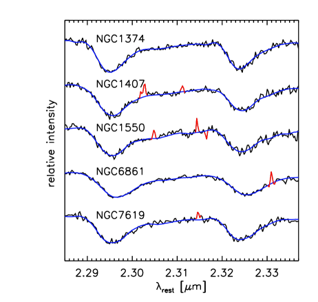
Figure 1: Examples of SINFONI spectra after spatial binning and continuum removal. For each galaxy above we display the spectrum derived from one of the central bins, with $\lambda_{\mathrm{rest}}$ denoting the rest-frame wavelength. The blue lines show the best fits, that are performed masking the red parts.

To avoid template mismatch, we chose only stars with equivalent width or line strength within the range of those derived from the galaxy spectra, i.e. we selected only stars that were representative of the stellar population of the galaxy. For this purpose, we used the line-strength index for the first CO band-head at 2.29 microns proposed by Mármol-Queraltó, Cardiel, Cenarro et al. (2008). This index definition has very little sensitivity to many aspects, most importantly S/N and velocity dispersion broadening (tested up to 400 km s^-1), which makes it well-suited for our work.

We derived the kinematics from the normalized spectra as follows. With the MPL method, an initial LOSVD was generated and then convolved with a linearly combined spectrum of template stars. The LOSVD and the weights of the template stars were iteratively adjusted until the convolved spectrum matched the galaxy spectrum, achieved by minimizing $\chi_{P}^{2}=\chi^{2}+\alpha P$, where $\alpha$ is the smoothing parameter and $P$, the penalty function, is the integral of squared second derivative of the LOSVD. To estimate the smoothing parameter, we created a large set of model galaxy spectra with an appropriate $\sigma$ and added varying amounts of noise to them. The smoothing required to recover the input LOSVD for each S/N was then used to infer the smoothing for the real galaxy spectra (see Appendix B of Nowak, Saglia, Thomas et al. (2008) for details).

The S/N was calculated after continuum normalisation as the inverse of the rms value obtained from the spectral fitting. For reliable kinematic results, we avoided having S/N smaller than 30 for each spatial bin. For an initial estimate of S/N we ran MPL using a fixed smoothing parameter for all spectra. The resulting fit (rms and thus the initial S/N) was then used to determine the appropriate smoothing parameter for each spectrum. When necessary, the binning was (re)adjusted to optimize the S/N.

The errors in the LOSVD were determined through a Monte Carlo simulation (Gebhardt et al., 2000b). The best-fitting combination of template spectra was convolved with the measured LOSVD and gaussian noise was added to create 100 different realizations of a galaxy spectrum. The LOSVDs of the realisations were measured and used to compute the 68 percent confidence interval. In Figs. 2-5, we present the two-dimensional kinematics of each galaxy, parametrised in the four Gauss-Hermite moments. The errors of the velocity and $\sigma$ measurements are about 10 km s^-1, while the uncertainties of $h_{3}$ and $h_{4}$ are around 0.02, on average.

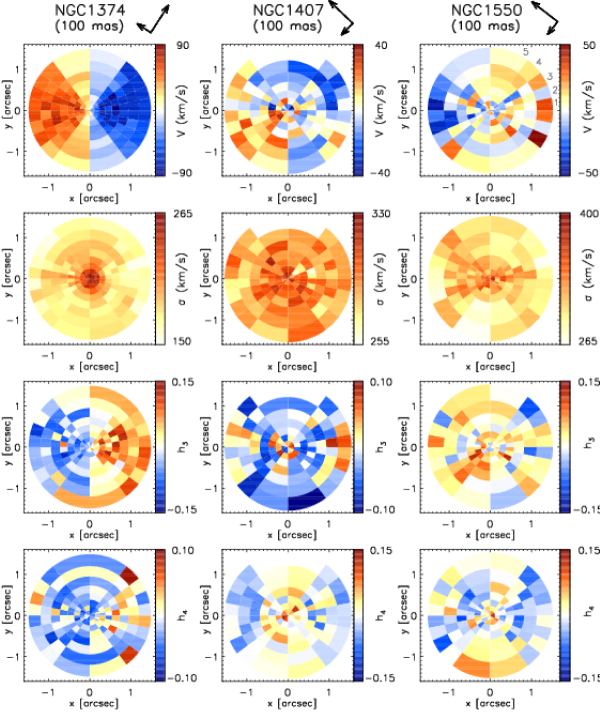
Figure 2: The two-dimensional kinematic maps of NGC 1374, NGC 1407 and NGC 1550, derived from SINFONI data and presented in terms of $V$, $\sigma$, $h_{3}$ and $h_{4}$. The major and minor axes of each galaxy are aligned with the abscissa and ordinate of the coordinate system. To identify the angular bins, we show the iv number in the velocity map of NGC 1550 with a grey color. The midpoint angles for iv=1 to iv=5 are 5.8^∘, 17.6^∘, 30.2^∘, 45.0^∘and 71.6^∘. The arrows next to the galaxy name indicate the North (long arrow) and East (short arrow) directions.

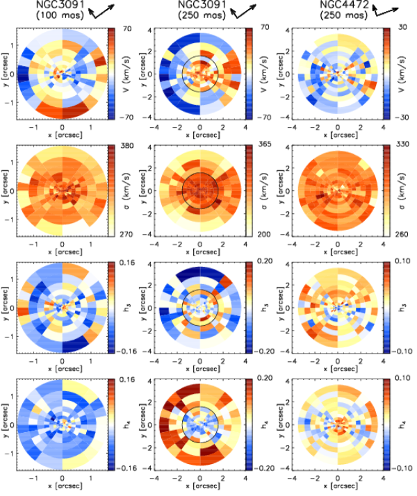
Figure 3: The same as Fig. 2 for NGC 3091 and NGC 4472. The scope of the 100-mas data of NGC 3091 is outlined in the 250-mas map (the black circle).

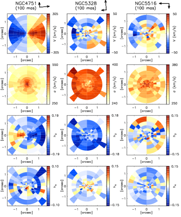
Figure 4: The same as Fig. 2 for NGC 4751, NGC 5328 and NGC 5516.

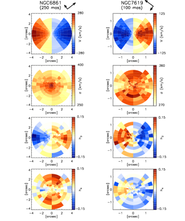
Figure 5: The same as Fig. 2 for NGC 6861and NGC 7619.

Four galaxies exhibit regular rotation: NGC 1374, NGC 4751, NGC 6861 and NGC 7619. In these galaxies, $h_{3}$ is anti-correlated with the rotational velocity, matching a widely observed trend (e.g. Bender, Saglia, & Gerhard 1994; Krajnović, Bacon, Cappellari et al. 2008; Krajnović et al. 2011; Fabricius, Saglia, Fisher et al. 2012). Of the four galaxies, NGC1374 has the lowest rotation; it also has the lowest velocity dispersion among the galaxies in the sample. The $\sigma$ profile of NGC 1374 shows a rather strong and clear gradient, peaking at around 260 km s^-1 in the center. NGC 4751 and NGC 6861 show the fastest rotation and the highest dispersion. A very steep gradient of $\sigma$ is seen in NGC 4751: from just below 500 km s^-1 in the center down to 250 km s^-1within the 1.5 arcsec radius. In NGC 7619, the velocity dispersion profile decreases more steeply along the major axis than along the minor axis and the majority of the LOSVDs are flat-topped as indicated by negative values in the $h_{4}$ map.

Five galaxies are dispersion-dominated with rotational velocity not more than 50 km s^-1 and no obvious rotation axis: NGC 1407, NGC 1550, NGC 4472, NGC 5328 and NGC 5516. In this group, NGC 1550, NGC 5328 and NGC 5516 have the highest $\sigma$, although none are higher than NGC 4751. In NGC 1550 and NGC 5516 $\sigma$ increases towards the centre, while in NGC 5328 it decreases. The $\sigma$ gradients in NGC 1407 and NGC 4472 are shallow. The lack of rotation in NGC 4472 is in agreement with van der Marel, Binney, & Davies (1990) who found no rotation within a radius of 5 arcsec.

For NGC 5328, the MPL fit yields a negative $h_{3}$ throughout the SINFONI FoV. This is atypical for early-type galaxies, regardless of whether they are rotating systems (where $h_{3}$ is usually anti-correlated with the velocity) or dispersion dominated systems ($h_{3}\sim 0$). With a systemic velocity of 4740 km s^-1, NGC 5328 has the largest redshift of all the galaxies in our sample. This means that the second CO bandhead is shifted into the red end of the SINFONI spectral range, which is significantly contaminated by residual OH emission. We therefore used only the first bandhead in the kinematic fitting. Given the single bandhead fit, we can not exclude the possibility that the negative $h_{3}$ may be the result of a faint sky emission line that is still strong enough to affect the extracted Gauss-Hermite moments. In the models, we therefore exclude the measured $h_{3}$ and $h_{4}$.

In some galaxies, like NGC 1407 and NGC 4472, one observes a slight trend for $h_{4}$ to increase towards the centre. In the analytical toy models of Baes, Dejonghe & Buyle (2005) (which, however, assume spherical symmetry and isotropy) $h_{4}$ tends to increase with the mass of the central black hole (relative to the rest of the system). However, the absolute values also depend on the steepness of the light profile and the increase in $h_{4}$ with the mass of the central black-hole is, even at central radii, not everywhere monotonic. It is therefore not clear if the observed central $h_{4}$ values are more indicative of the orbital or of the mass structure in the centres of the galaxies.

NGC 3091 displays a signature of a kinematically decoupled core. The stars at $r<1$ arcsec appear to be rotating in the opposite direction from the stars at larger radii. The $h_{4}$ within $\sim$1.5 arcsec is predominantly negative, but becomes positive outside this radius, which provides another evidence for a decoupled core. The 100-mas and 250-mas datasets for NGC 3091 overlap in the inner 1.5 arcsec radius. For the purpose of the modelling, we used only the data with higher spatial resolution up to the 6th radial bin ($r<0.65$″) and used the 250-mas data to cover the region with 0.65″$<r<$ 4″.

In Fig. 6 we show the $\lambda_{R}$ parameter of Emsellem, Cappellari, Krajnović et al. (2007) for our galaxies. A global classification into slow and fast rotators based on this plot is difficult due to the small field of view (e.g. Emsellem, Cappellari, Krajnović et al. 2011). Note also, that the field of view is not much larger than the PSF, which affects the derived $\lambda_{R}$ as seen clearly for NGC 3091.

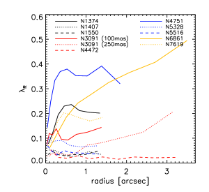
Figure 6: The $\lambda_{R}$ parameter of Emsellem, Cappellari, Krajnović et al. (2007) for the sample galaxies.

3.2 Additional kinematics

In addition to the SINFONI data, we used a set of ground-based kinematic data at larger radii for the dynamical modeling of each galaxy. These data were necessary to get a good handle on $\Upsilon$ and DM. Most of the datasets came in the form of long slit data and were taken from the literature. All these auxiliary data were available in the form of Gauss-Hermite moments with the respective errors. From these moments, we constructed the LOSVDs with the uncertainties measured through 100 Monte Carlo realizations. We used these LOSVDs in the modeling.

NGC 1374. The auxiliary dataset for this galaxy is long slit data along the major axis (up to $\sim$20 arcsec) taken with the EMMI spectrograph at the ESO NTT. For the details on the observation, reduction and the kinematic analysis, see Appendix A. There are other long slit data available in the literature, i.e. Longo, Zaggia, Busarello et al. (1994) and D’Onofrio, Zaggia, Longo et al. (1995). We did not attempt to include these data because they did not provide $h_{3}$ and $h_{4}$ information and the data were less extended than the long-slit data that we use in this work.

NGC 1407. We used the slit data from Spolaor et al. (2008a), who provided kinematics along the major axis up to 40 arcsec, a little more than 0.5$R_{e}$.

NGC 1550. We used long-slit kinematic data from Simien & Prugniel (2000), who provided only $V$ and $\sigma$ measurements. Using this dataset, we generated LOSVDs by setting $h_{3}$ and $h_{4}$ to zero with uncertainties of 0.1, allowing the models some extra freedom in fitting the LOSVD without biasing them into negative or positive $h_{3}$ and $h_{4}$ values. These data extend out to 26 arcsec along the major axis. The slit was placed at a position angle of 38^∘. The SINFONI data was adjusted to this PA to align the slit with the photometric major axis.

NGC 3091. For this galaxy, we obtained a set of new IFU data using VIRUS-W at the McDonald 2.7m telescope (see Appendix B). Each fiber has a size of 3.14 arcsec in diameter, much larger than the model bin size in the central 10 arcsec. We therefore ignored the data inside 10 arcsec. Since SINFONI data are available only out to 4 arcsec, the region between 4 and 10 arcsec is not covered by any data. Between 10 and 50 arcsec, where the S/N is sufficiently good, we averaged the spectra of the fibers that fell on the same model bin and derived the kinematics from these spectra. The VIRUS-W data was binned into radial and angular bins, like the SINFONI data.

NGC 4472. We used long slit data from Bender, Saglia, & Gerhard (1994), who presented kinematics of NGC 4472 out to $\sim 75$ arcsec along the major axis and out to 60 arcsec along the minor axis.

NGC 4751. As complementary data, we used an IFU dataset obtained using the Wide-Field Spectrograph WiFeS at the Siding Spring ANU 2.3m telescope (see Appendix C). In the modeling, the WiFeS datapoints were treated as multiple slits across the central part of the galaxy. They were parallel to each other and did not align with the major or minor axis. Due to the axisymmetry assumption we folded the four quadrants of the galaxy; LOSVDs with identical spatial position in the folded quadrant were averaged. This resulted in two sets of slit data which were different in spatial orientations. The first set of slits was positioned at an angle of 5^∘ and the second one at -5^∘, measured counter-clockwise (positive sign) from the major axis, each having 5 and 4 pseudo-slits, respectively (see Fig. 7 for clarity). WiFeS data overlapping with the SINFONI data were excluded from the orbit modelling.

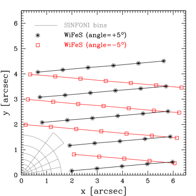
Figure 7: Spatial orientation of SINFONI and WiFeS datapoints in the folded quadrant of NGC 4751. The x and y-axes correspond to the abscissa and ordinate in Fig. 4. The grey lines outline the SINFONI bins. WiFeS datapoints are plotted as asterisks and rectangles, connected by solid lines with the corresponding colors to depict the “pseudoslits”. The red lines show the pseudoslits positioned at an angle of -5^∘and the black lines outline those the angle of 5^∘.

NGC 5328. As for NGC 3091 we obtained new IFU data using VIRUS-W (see Appendix B). But in this case we employed a Voronoi binning scheme which yields a median S/N per Å  of 25. The bins cover a region out to about 30 arsec along the major and out to 20 arcsec along the minor axis. The binning is illustrated in Fig. 8.

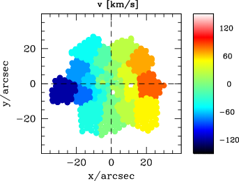
Figure 8: The velocity field of NGC 5328 as observed with VIRUS-W.

NGC 5516. The extended kinematic data for this galaxy were also observed using WiFeS (Appendix C). The data used in the model were limited up to 7 arcsec. Outside this radius the S/N was low, giving unreasonable kinematic moments or uncertainties. The WiFeS data were treated and folded in the same way as for NGC 4751. The two sets of “pseudo-”slit data were at angles of 72^∘ and 108^∘, measured counter-clockwise from the major axis. Each set consists of five parallel slits (see Fig. 9). We did not include WiFeS datapoints located inside the SINFONI FoV in the dynamical modelling.

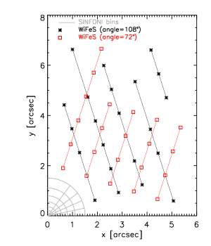
Figure 9: The same as Fig. 7 for NGC 5516. The red lines show the pseudoslits positioned at an angle of 72^∘and the black lines outline those at the angle of 108^∘.

NGC 6861. The additional dataset for this galaxy is long slit data along the major axis (up to $\sim$10 arcsec) taken using the EMMI spectrograph. For the details on the observation, reduction and the kinematic analysis, see Appendix A.

NGC 7619. For this galaxy, we used the kinematic data from Pu, Saglia, Fabricius et al. (2010) who provided $V$, $\sigma$, $h_{3}$ and $h_{4}$ out to 60 arcsec, almost twice the $R_{e}$, along both the major and minor axes. The spatial distribution of the original datapoints was dense, slowing down the computation while not increasing the significance of the results. We therefore spatially rebinned the data to create a dataset with fewer data points and used this in the modeling.

4 Light distribution

To put constraints on the spatial distribution of stars we performed surface photometry and deprojected this 2D information into a light density distribution. The deprojection was done axisymetrically using the code of Magorrian (1999). The seeing correction was included in the deprojection as described in Rusli, Thomas, Erwin et al. (2011), using a multi-gaussian profile as a representation of the actual PSF. We adopted an inclination of 90^∘ for each galaxy, unless stated otherwise (see Fig. 11)

For two galaxies, we used the photometry that was already available in the literature: the photometry for NGC 7619 was taken from Pu, Saglia, Fabricius et al. (2010), while for NGC 4472 we used the photometry published in Kormendy, Fisher, Cornell et al. (2009). We describe the photometry of the other galaxies below.

4.1 The photometry of NGC 1374

We used an HST image taken with ACS-WFC and the F475W filter (Proposal ID: 10911, PI: Blakeslee), and also an NTT EMMI image available from the ESO archive and taken with the filter ”SPEC RS” (Program ID: 56.A-0430, PI: Macchetto/Giavalisco). We calibrated the final profile to the B band, using the aperture photometry of Caon, Capaccioli, & D’Onofrio (1994). The isophotal analysis was carried out using the software of Bender & Moellenhoff (1987). The matching between the HST and the ground-based profiles was performed in the region $5<a<20$ arcsec, where $a$ is the semi-major distance from the center, and we used the ground-based profile for $a>20$ arcsec. The matching procedure (used also for all the following galaxies) consists in determining the scaling and sky value that minimize the magnitude square differences between the two profiles, assuming that the ground-based profile has the correct sky subtraction performed. (Determining the sky background value for the HST image in this fashion is necessary when the galaxy fills the HST FoV.) The rms residuals in the region of the matching are small, typically 0.01-0.02 mag. The appropriate PSF to use for deprojecting the photometry is that of the ACS/WFC. We used the TinyTim program, which for the ACS/WFC generates an “observed” (i.e., optically distorted) PSF. Since the isophotal analysis was performed on the distortion-corrected “drizzled” image, we applied the same process to the PSF image, using custom-written Python code. The PSF image output by TinyTim was copied into the flat-fielded (but still distorted) ACS/WFC image, replacing the center of the galaxy. The full image was then run through the same multidrizzle processing to produce a distortion-corrected WFC mosaic. The processed PSF was then cut out from the mosaic. To generate the PSF image with the TinyTim software, we used the position of the galaxy center on the detector and a K giant spectrum as input (also for the galaxies below when TinyTim is used).

4.2 The photometry of NGC 1407

We used an HST image taken with ACS/WFC and the F435W filter (Proposal ID: 9427, PI: William Harris) and a ground-based B-band image taken at the 40-inch telescope in Siding Spring equipped with the wide field imager. On 2001 October 19 we took 6 pointings, each with a 10-minute exposure. The images were reduced and combined using IRAF. The isophotal analysis was performed using the software of Bender & Moellenhoff (1987). The ground-based surface brightness profile was calibrated using photoelectric photometry of Burstein et al. (1987). We matched the HST profile to the ground-based data in the region $5<a<20$ arcsec, where $a$ is the semi-major axis of the galaxy, and merged the two dataset using the matched HST profile for $a<20$ arcsec. The PSF used in the deprojection was generated using the TinyTim and passed through the drizzle software.

4.3 The photometry of NGC 1550

We used an image from the Isaac Newton Telescope’s Wide Field Camera (INT-WFC), originally observed by Michael Pohlen. The observation was a 300 second exposure in the Sloan $r$ filter, taken on 2003 December 15; the pixel scale was 0.331 arcsec/pixel and the median seeing FWHM was 1.4 arcsec. We calibrated it to the Cousins $R$ using aperture photometry provided by Djorgovski (1985). Since there are no HST images of this galaxy, we used our $K$-band SINFONI image (generated by collapsing the reduced SINFONI datacube along the wavelength direction) for higher resolution in the central region of the galaxy. We perfomed the isophotal analysis on both images using the software of Bender & Moellenhoff (1987) and matched the SINFONI surface brightness profile to the ground-based profile in the region $0.8<a<1.6$ arcsec. The combined profile uses the SINFONI data at $a<1$ arcsec and the ground-based data for $a>1$ arcsec. The SINFONI PSF was used in the deprojection.

4.4 The photometry of NGC 3091

We used an HST ASC/WFC images taken using the F814W filter (Proposal ID: 10787, PI: Charlton). We calibrated them to the Cousins $I$ using the approach of Sirianni, Jee, Benítez et al. (2005) with the updated zero points available at the STSCI website, along with colors from the galaxy photometry compilation of Prugniel & Heraudeau (1998). Comparison with the aperture photometry of Reid, Boisson, & Sansom (1994) shows that there is a -0.03 mag difference to the Cousins I system. The isophotal analysis was performed using the software of Bender & Moellenhoff (1987). The PSF used in the deprojection was generated using the TinyTim software (Krist et al., 2011) and passed through the drizzle software.

4.5 The photometry of NGC 4751

We used an HST image taken with the NICMOS2 imager and the F160W filter (Proposal ID: 11219, PI: Alessandro Capetti) and a ground-based R-band image taken at the ESO-MPG 2.2m telescope in La Silla equipped with the wide field imager (WFI). The ground-based data (4 exposures of 5 minutes each) were taken on 2010 July 8. They were reduced (as all the WFI images described below) using the mupipe software developed at the University Observatory in Munich (Gössl & Riffeser, 2002). After the initial bias and flat-field corrections, cosmic rays and bad pixels were masked, and the images were resampled to a common grid and stacked. A constant sky value was estimated from empty regions distant from the galaxy and subtracted from the stacked image. The calibration was performed using the photoelectric aperture photometry in the R band of Poulain & Nieto (1994). The HST profile was matched to the ground-based one in the region $2^{\prime\prime}<a<5^{\prime\prime}$, and used for $a<5^{\prime\prime}$. The PSF was generated using TinyTim.

4.6 The photometry of NGC 5328

We used the 60sec exposure EFOSC2 image taken at the 3.6m ESO telescope with the R filter (Grützbauch et al., 2005) that we downloaded from the archive. After the standard reduction, the calibration was performed using the photoelectic photometry in the V band from Hyperleda. Since there are no HST images of this galaxy, we used our $K$-band SINFONI image (generated by collapsing the reduced SINFONI datacube along the wavelength direction) for higher resolution in the central region of the galaxy. We perfomed the isophotal analysis on both images using the software of Bender & Moellenhoff (1987) and matched the SINFONI surface brightness profile to the ground-based profile in the region $0.8\arcsec<a<1.9\arcsec$. The combined profile uses the SINFONI data at $a<1.2\arcsec$ and the ground-based profile ground-based data for $a>1.2\arcsec$. The SINFONI PSF is used in the deprojection.

4.7 The photometry of NGC 5516

We used an HST image taken with the PC of WFPC2 and the F814W filter (Proposal ID: 6579, PI: John Tonry) and a ground-based R-band image taken at the ESO-MPG 2.2m telescope in La Silla equipped with the Wide Field Imager. The ground-based data (4 exposures of 230 seconds each) were taken on 2010 July 10 and were reduced as for NGC 4751. The calibration was performed using the photoelectric photometry in the R band from Poulain & Nieto (1994). The HST profile was matched to the ground-based one in the region 3 arcsec $<a<$ 10 arcsec, and used for $a<8.9$ arcsec. The PSF was generated using TinyTim.

4.8 The photometry of NGC 6861

We used an HST image taken with WFPC2 and the F814W filter (Proposal ID: 5999, PI: Andrew Philip) and a ground-based R-band image taken at the ESO-MPG 2.2m telescope in La Silla equipped with the wide field imager. The ground-based data (4 exposures of 230 seconds each) were taken on 2010 July 13 and were reduced as for NGC 4751 and NGC 5516. We calibrated the HST profile of the Cousins I-band using the measured (F555W-F814W) colour and the equations of Holtzman, Burrows, Casertano et al. (1995). We matched the ground-based profile to the HST one in the region $10^{\prime\prime}<a<85^{\prime\prime}$ and used the profile at $a>21.3^{\prime\prime}$. The PSF was generated using TinyTim.

5 Dynamical models

The dynamical modeling was performed using the axisymmetric orbit superposition technique (Schwarzschild, 1979), described in Gebhardt et al. (2000b), Thomas, Saglia, Bender et al. (2004) and Siopis et al. (2009). This technique was implemented as follows. First, the gravitational potential was calculated from the prescribed total mass distribution using the Poisson equation. This total mass distribution is defined as $\rho=\Upsilon\times\nu+M_{\mathrm{BH}}\times\delta(r)+\rho_{\rm DM}$ where $\Upsilon$ is the mass-to-light ratio of the stars, $\nu$ is the luminosity density distribution of the stars and $\rho_{\rm DM}$ is the dark halo density. Then, thousands of time-averaged stellar orbits were generated in this potential. Each of their weights was calculated such that the orbit superposition reproduced the luminosity density and fitted the kinematics as good as possible. For each potential we calculated about 24,000 orbits. We derived the best-fitting set of parameters by setting up a parameter grid in the modeling, with each gridpoint representing a trial potential. The best-fit model was chosen based on the $\chi^{2}$ analysis. For all galaxies except NGC 5328 the $\chi^{2}$ is computed by comparing the LOSVDs derived by the model to the measured non-parametric LOSVDs and their uncertainties.

As described above (Sec. 3.1), the shapes of the SINFONI LOSVDs for NGC 5328 might be systematically affected by a faint sky emission line and we consider only the measured $V$ and $\sigma$ to be reliable. When we compute the $\chi^{2}$ difference between the models and the SINFONI data, we therefore do not use the full LOSVDs. Instead, for each model bin with SINFONI data we compute the Gauss-Hermite moments $h_{1},\ldots,h_{4}$ of the respective model LOSVD. The series expansion is done based on the measured $V$ and $\sigma$, rather than using the values of the corresponding best-fitting Gaussian to the model LOSVD. Hence, $h_{1}$ and $h_{2}$ will be non-zero unless a Gaussian fit to the model LOSVD yields the measured $V$ and $\sigma$. For the comparison between model and SINFONI data we therefore calculate the $\chi^{2}$-difference in $h_{1}$ and $h_{2}$, using $h_{1}=h_{2}=0$ as “data” (e.g. Cretton et al. 1999). The corresponding errors $dh_{1}$ and $dh_{2}$ were derived from the measured $dV$ and $d\sigma$ through MC simulations. Leaving all the $h_{n}$ unconstrained for $n>2$ results in unrealistically noisy model LOSVDs. To reduce the noise, we extend the $\chi^{2}$-sum over $h_{3}$ and $h_{4}$ as well. However, the measured $h_{3}$ and $h_{4}$ are likely biased (Sec. 3.1) and instead of trying to reproduce them by a model fit, we use $h_{3}=h_{4}=0$ as “data”. We artificially increase the uncertainties to $dh_{3}=dh_{4}=0.1$, in order not to bias the models too strongly towards any particular values, while still keeping them within a plausible range. In early-type galaxies, $\pm 0.1$ is the typical range of observed $h_{3}$ and $h_{4}$. Using $h_{1}$ to $h_{4}$ for the $\chi^{2}$ as described above allows us to constrain the models towards the observed $V$ and $\sigma$ with reasonably smooth LOSVDs, but without a strong bias towards any particular LOSVD shape, as parameterised by $h_{3}$ and $h_{4}$. The best-fitting $V$, $\sigma$, $h_{3}$ and $h_{4}$ are shown in Fig. 26. For the outer VIRUS-W data, we compare model and data using the full LOSVDs as for the other galaxies.

Along with the axisymmetry assumption in the modeling, we folded the four quadrants of each galaxy into one. For the SINFONI and VIRUS-W data, the folding was done by averaging the LOSVDs of four bins at the same angular and radial position. For the slit data, we fitted both sides of the slit simultaneously. The Voronoi binning of NGC 5328 is not axisymmetric and we fit the four quadrants independently, using the sum of the four $\chi^{2}$ in the final analysis.

5.1 The Importance of DM in the modeling

The degeneracy between $M_{\rm BH}$ and $\Upsilon$ is often a problem in $M_{\rm BH}$ measurements. It is evident when the two-dimensional $\chi^{2}$ distribution (as a function of $M_{\rm BH}$ and $\Upsilon$) appears diagonal (e.g. Gültekin, Richstone, Gebhardt et al. 2009; Nowak, Thomas, Erwin et al. 2010, Schulze & Gebhardt 2011). It is thought that placing more stringent constraints on $\Upsilon$ will help to pin down the black hole mass more accurately. To do this, the naive approach would be to provide as much/extended data as possible to constrain $\Upsilon$. We show here that this strategy is not advisable when DM is neglected in the models.

From the slit data of NGC 1407, NGC 4472 and NGC 7619, we created multiple sets of data for each galaxy by truncating the slit data at different outer radii ($r_{\rm trunc}$). For each galaxy, we ran models using these kinematic datasets and also the full dataset to determine $\Upsilon$ without having DM present in the model ($\rho_{\rm DM}$ is zero). $M_{\rm BH}$ was set to zero. Fig. 10 plots the $\Delta\chi^{2}$ vs. $\Upsilon$ obtained from these runs for each of the three galaxies, $\Delta\chi^{2}$ being the difference between $\chi^{2}$ of each model and the minimum $\chi^{2}$ of the run. As a comparison, we also show the $\Delta\chi^{2}$ distribution when DM is included in the models for the run with the full dataset (described in Section 5.2). The $\Upsilon$ values along the x-axis are normalized by the best-fit $\Upsilon$ obtained from the run with DM ($\Upsilon$ with $\Delta\chi^{2}=0$ along the black line). The red line shows the run without DM, but using the full slit data, i.e. the same kinematic dataset as the run with DM. The blue and green represent the runs without DM, with decreasing $r_{\rm trunc}$.

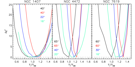
Figure 10: The $\Delta\chi^{2}$ distribution as a function of $\Upsilon$. The $\Upsilon$ values are all normalized by the best-fit $\Upsilon$ obtained from modeling with DM (black line). The red, blue and green lines are models without DM, with different $r_{\rm trunc}$. The value of $r_{\rm trunc}$ for each run is written in the plot.

It can be seen for each of the three galaxies in Fig. 10 that the highest and lowest values of the best-fit $\Upsilon$ were found when the full kinematic dataset was used: the $\Upsilon$ is lowest when DM is included and is highest when DM is omitted. For the case without DM, $\Upsilon$ increases as $r_{\rm trunc}$ gets larger. This is expected because more spatially extended data go farther into the region where DM is dominant. In the modeling, omitting the DM component requires $\Upsilon$ to increase in order to compensate for the missing dark mass. The larger $r_{\rm trunc}$ is, the more dark mass there is which must be compensated for, thereby increasing $\Upsilon$ further. The situation is worsened by the fact that the 1$\sigma$ error bars of $\Upsilon$ ($\Delta\chi^{2}=1$) decrease with increasing $r_{\rm trunc}$. When more extensive data are used, the $\chi^{2}$ curve becomes steeper, excluding the “true” $\Upsilon$ (with DM) with a higher confidence. For the three galaxies, this systematic bias appears to be as large as $\sim$20-30 percent.

It is clear that omitting DM in the modeling biases $\Upsilon$. In principle, this bias in $\Upsilon$ could also affect the black hole mass due to the degeneracy. It is therefore important to consider DM in the modeling to investigate how much effect this bias has on $M_{\rm BH}$. We discuss this further in Section 7. In the following Section, we describe how we incorporate DM in the modeling to fit $M_{\rm BH}$.

5.2 Inclusion of DM in the Model

We used a spherical cored logarithmic (LOG) dark halo profile (Binney & Tremaine, 1987). As found in Gebhardt & Thomas (2009) and McConnell et al. (2011a), the exact shape of the dark halo is of little importance to the black hole mass and in most cases the LOG halo gives a better fit compared to the other commonly used profiles. Since our aim is to constrain $M_{\rm BH}$ and not the dark halo, we avoid a detailed study of the halo parameters. The LOG halo is given by

$$\rho_{\rm LOG}(r)=\frac{V_{c}^{2}}{4\pi G}\frac{3r_{c}^{2}+r^{2}}{(r_{c}^{2}+r^{2})^{2}}$$ (1)

where $r_{c}$ is the core radius, within which the density slope of the DM is constant, and $v_{c}$ is the asymptotic circular velocity of the DM. When the dark halo is present in the model, there is a total of four free parameters ($\Upsilon$,$M_{\rm BH}$, $V_{c}$ and $r_{c}$) to be determined.

Calculating models to determine all four parameters simultaneously is computationally expensive. It requires about $\sim$ 100,000 models per galaxy and until now such an analysis has only been carried out for four galaxies: M 87 (Gebhardt & Thomas, 2009), NGC 4649 (Shen & Gebhardt, 2010), NGC 4594 (Jardel et al., 2011) and NGC 1277 (van den Bosch et al., 2012). Most of the recent studies considering DM for dynamical $M_{\rm BH}$ determinations used a fixed (or a handfull of fixed) DM halos (e.g. Schulze & Gebhardt 2011, McConnell et al. 2011a; McConnell, Ma, Murphy et al. 2012). This lowers the computational effort since only $M_{\rm BH}$ and $\Upsilon$ are varied. However, to a certain extent a lower (higher) $\Upsilon$ can be compensated for by a more (less) massive halo. A fixed halo may therefore artificially narrow down the range of $\Upsilon$ consistent with the data, and, moreover, bias it towards a certain value. This, in turn, can affect the derived $M_{\rm BH}$ and its uncertainties. In order to avoid such a possible bias, but still keep the computational effort feasible for our sample of ten galaxies, we here take an intermediate approach.

We first calculate models without the central, high-resolution SINFONI data. In this run we set $M_{\rm BH}$ to zero and vary $V_{c}$, $r_{c}$ and $\Upsilon$. We do not use the central SINFONI data since it probes the black hole. From this first set of models we determine the best-fitting $V_{c}$ and $r_{c}$ for each $\Upsilon$. We then proceed to determine the best-fit $M_{\rm BH}$ (Section 6) by varying $M_{\rm BH}$ and $\Upsilon$  using the best-fit $r_{c}(\Upsilon)$ and $V_{c}(\Upsilon)$ for each $\Upsilon$ as calculated in the first step. In this way, we reduce the computational load and time quite significantly, but still allow the DM distribution to adapt to different $\Upsilon$.

Fitting the dark halo can be done only when the kinematic data are sufficiently extensive, which is not always the case. For galaxies with limited data, we skipped the first step and we directly determined $M_{\rm BH}$ and $\Upsilon$ by fixing $r_{c}$ and $V_{c}$ to values from dark matter scaling relations which were derived from a sample of Coma galaxies (Thomas, Saglia, Bender et al., 2009). The relations are written as follows:

$${\rm log}\,r_{c}=1.54+0.63({\rm log}(L_{B}/L_{\odot})-11.0)$$ (2)

$${\rm log}\,V_{c}=2.78+0.21({\rm log}(L_{B}/L_{\odot})-11.0)\\$$ (3)

with $r_{c}$ and $V_{c}$ stated in kpc and km s^-1 respectively. The galaxy luminosity $L_{B}$ is calculated from the B-band absolute magnitude given in Table 1. These equations are used to assign $r_{c}$ and $V_{c}$ values for NGC 1374, NGC 1550 and NGC 5516.

The best-fitting $r_{c}$ and $V_{c}$ for all galaxies with fitted halo are presented in Table 3. They are not the exact values expected from the dark matter scaling relations, but they fall within the scatter. For galaxies with long slit data, we included all the slit datapoints to fit the dark halo. For NGC 3091, we used the VIRUS-W data and the outer part of SINFONI 250-mas data because the VIRUS-W data started only at 10 arcsec. These VIRUS-W data were advantageous because of the larger spatial coverage, but they did not deliver useful results when used by themselves. Modeling $\Upsilon$ and DM by using only the VIRUS-W data resulted in a rather flat $\chi^{2}$ distribution for $\Upsilon$. We therefore included the 250-mas SINFONI data as well, but only used datapoints outside 1 arcsec.

6 Black hole masses

Table 3: The best-fit $M_{\rm BH}$ and $\Upsilon$ with and without DM

Galaxy	$M_{\rm BH,NoDM}$	$\Upsilon_{\rm NoDM}$	$M_{\rm BH,DM}$	$\Upsilon_{\rm DM}$	$r_{c}$	$V_{c}$	${\rm D_{SoI}}$	band
	($M_{\odot}$)		($M_{\odot}$)		(kpc)	(km s-1)	(″)
NGC 1374 †	$5.8(5.3,6.3)\times 10^{8}$	$5.7(5.3,6.1)$	$5.8(5.3,6.3)\times 10^{8}$	$5.3(4.7,5.9)$	6.0	336	1.54	B
NGC 1407	$3.8(2.4,4.4)\times 10^{9}$	$10.7(9.7,11.7)$	$4.5(4.1,5.4)\times 10^{9}$	$6.6(5.8,7.5)$	10.9	340	3.89	B
NGC 1550 †	$3.7(3.3,4.2)\times 10^{9}$	$4.3(3.9,4.7)$	$3.7(3.3,4.1)\times 10^{9}$	$4.0(3.4,4.5)$	20.7	507	1.34	R
NGC 3091	$9.7(8.1,11.0)\times 10^{8}$	$5.4(5.2,5.7)$	$3.6(3.4,3.7)\times 10^{9}$	$3.8(3.6,4.1)$	29.8	809	1.21	F814W
NGC 4472	$1.7(1.0,2.0)\times 10^{9}$	$7.3(6.9,7.7)$	$2.5(2.4,2.8)\times 10^{9}$	$4.9(4.5,5.3)$	13.6	780	3.00	V
NGC 4751	$1.4(1.3,1.5)\times 10^{9}$	$13.1(12.7,13.4)$	$1.4(1.3,1.5)\times 10^{9}$	$12.2(11.5,12.8)$	5.2	300	0.70	R
NGC 5328	$4.8(1.7,8.0)\times 10^{7}$	$10.1(9.9,10.4)$	$4.7(2.8,5.6)\times 10^{9}$	$4.9(4.3,5.5)$	18.6	400	1.34	V
NGC 5516 †	$3.2(3.1,3.4)\times 10^{9}$	$5.6(5.5,5.8)$	$3.3(3.0,3.5)\times 10^{9}$	$5.2(5.1,5.5)$	31.8	585	1.06	R
NGC 6861	$2.2(2.1,2.4)\times 10^{9}$	$5.9(5.7,6.1)$	$2.0(1.8,2.2)\times 10^{9}$	$6.1(6.0,6.3)$	21.8	200	0.76	I
NGC 7619	$4.2(3.0,5.5)\times 10^{8}$	$5.2(4.9,5.6)$	$2.5(2.2,3.3)\times 10^{9}$	$3.0(2.6,3.3)$	39.2	700	0.83	I

In this Section we present the best-fitting black hole masses along with the $\Upsilon$ values that are derived from the dynamical modeling. In addition to the high-resolution SINFONI data, we also included the other ground-based data at larger radii (Section 3.2). When the DM was included in the model, we used either the best-fit LOG halos as a function of $\Upsilon$ or a fixed halo according to the B absolute magnitude taken from HyperLeda (equations 2 and 3). We also ran models without DM, fitting only $M_{\rm BH}$ and $\Upsilon$ and using the same kinematic dataset as the runs with DM. Table 3 shows the results with the corresponding 1$\sigma$ uncertainties. The size of the sphere of influence, calculated based on $M_{\rm BH}$ with DM and the central $\sigma$ taken from HyperLeda, is also listed in that table. We include $r_{c}$ and $V_{c}$ for the galaxies in which we use a fixed halo. The Gauss-Hermite fit of the best-fitting model to the data for each galaxy is shown in Appendix D (Figs. 19-30).

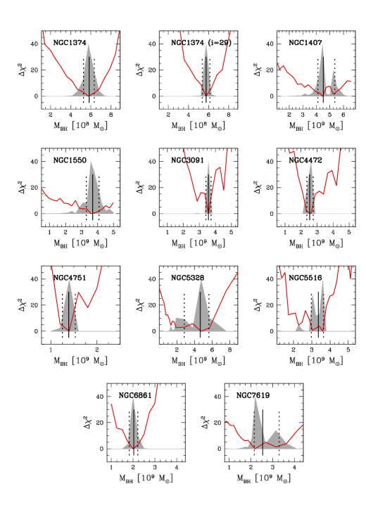
Figure 11: $\Delta\chi^{2}$ (red lines) and marginalized likelihood $P$ (shaded, cf. equation 4) vs $M_{\rm BH}$ for models with DM. The likelihood is scaled arbitrarily to a maximum value of $40$ in each panel. For NGC 1374, we show the plot for two inclinations. The vertical full lines show the derived black hole masses; the vertical dashed lines the 1$-\sigma$ errors (see Table 3).

In Fig. 11 we plot the $\chi^{2}$ distribution as a function of $M_{\rm BH}$ (marginalized over $\Upsilon$ and also over $r_{c}$ and $V_{c}$ in some cases) for each galaxy, when DM is included. For some galaxies, these profiles look noisier than for others and the noise does not necessarily decrease with increasing grid resolution. The profiles of galaxies with a larger rotation over velocity dispersion ratio, like NGC 1374 and NGC 7619, seem to be smoother. In spite of the noise, each profile does show a clear minimum.

We obtain the $M_{\rm BH}$ and their uncertainties from the cumulative of the marginalized likelihood distribution

$$P(M_{\mathrm{BH}})\propto\sum\exp\left[-\frac{1}{2}\Delta\chi^{2}(M_{\mathrm{BH}},\Upsilon)\right]\delta\Upsilon,$$ (4)

where the sum extends over all sampled $\Upsilon$ (e.g. McConnell et al. 2011a). Another common approach is to derive $M_{\rm BH}$ from the minimum of $\chi^{2}$ and the uncertainties from $\Delta\chi^{2}=1$. In our case, either approach gives similar results. Fig. 11 shows also $P$ for all galaxies.

Longo, Zaggia, Busarello et al. (1994) and D’Onofrio, Zaggia, Longo et al. (1995) suggest that NGC 1374 might be a face-on misclassified lenticular, based on the kinematic profile derived from their long-slit data. For this reason, we additionally ran models with an inclination of 29^∘; with this inclination, the projected flattening ($b/a$; $a$ and $b$ are the semi major and semi minor axes radius) of 0.88 translates into an intrinsic flattening of 0.25 (disk-like). We show the results in Fig. 11. We see that changing the inclination to i=29 hardly changes $M_{\rm BH}$ and $\Upsilon$. The same is true when the galaxy is modeled without DM. $M_{\rm BH}$ and $\Upsilon$ in this galaxy seem to be robust against DM inclusion and a change of inclination.

Despite the steep change in $\Upsilon$between models with and without DM, the $M_{\rm BH}$ in NGC 1407 stays almost the same. The black hole mass measured for this galaxy is $4.3\times 10^{9}$ $M_{\odot}$, comparable to $M_{\rm BH}$ in NGC 4649 which has a higher velocity dispersion of around 350 km s^-1 (Shen & Gebhardt, 2010). NGC 1407 has the highest $M_{\rm BH}$ in the sample, although the velocity dispersion is rather low. In NGC 5328, the $M_{\rm BH}$ without DM is too small to be formally resolved; without DM, only an upper limit for $M_{\rm BH}$ can be derived.

There are two sets of SINFONI data for NGC 3091, which overlap in the inner 1.5 arcsec radius. The 100-mas dataset excels in spatial resolution while 250-mas data is better in S/N. To fit $M_{\rm BH}$  we use the 100-mas data out to a radius of 0.65 arcsec, which corresponds to the 6th radial bin in the kinematic maps. With $M_{\rm BH}$ of $3.6\times 10^{9}$$M_{\odot}$, the radius of the sphere of influence is 0.68 arcsec, meaning that the region within the sphere of influence is fully constrained by the high-resolution data (100-mas). Outside this radius (out to $\sim 4$ arcsec) the kinematics is provided by the 250-mas data.

7 The change of $M_{\rm BH}$ due to DM

In three out of our ten galaxies, $M_{\rm BH}$ stays the same or changes only within the $1\sigma$ errors when a DM halo is included. In one galaxy, NGC 6861, $M_{\rm BH}$ decreases (but still being slightly above the upper limit of Beifiori et al. 2009). However, the confidence intervals for models with and without DM are nearly identical for this galaxy. There are three galaxies whose black hole masses change significantly outside their $1\sigma$ errors, i.e. NGC 3091, NGC 5328 and NGC 7619. Without considering NGC 5328 (see above), $M_{\rm BH}$ increases by a factor of 2 on average when a DM halo is included. This is similar to the increase in $M_{\rm BH}$ found for M87 (Gebhardt & Thomas, 2009), but larger than that found by Schulze & Gebhardt (2011) using their sample of 12 galaxies.

Gebhardt et al. (2011) suggest two strategies for deriving an accurate $M_{\rm BH}$. These are to get $\Upsilon$ right in the first place or to have high resolution data that cover the central region of the galaxy. Both strategies have been tested on M87 by Gebhardt & Thomas (2009) and Gebhardt et al. (2011). Below we address how these two strategies apply to our sample galaxies.

7.1 The influence of data resolution

We show a plot of spatial resolution vs the change in $M_{\rm BH}$ in Fig. 12. $D_{\rm res}$ is the diameter of the resolution element, which is largest of the aperture size, seeing, the PSF FWHM and the model bin size. For our galaxies, $D_{\rm res}$ represents the PSF FWHM (last column in Table 2), except for NGC 1407 where we use the average size of the model bins inside the SINFONI FOV, i.e. 0.24 arcsec (larger than the PSF FWHM of 0.19 arcsec). The velocity dispersion values from HyperLeda ($\sigma_{0}$ in Table 1) were used to derive $D_{\rm inf}$, the diameter of the sphere of influence. We have checked that for the ten galaxies in our sample, the velocity dispersions from spatially-averaged SINFONI spectra are similar to these. Using these SINFONI $\sigma$ values, or the $\sigma_{e}$ values from Table 1, does not change the appearance of the plot. $D_{\rm inf}$ is calculated using $M_{\rm BH}$ without dark matter. We include M87 (Gebhardt & Thomas, 2009; Gebhardt et al., 2011), NGC 4649 (Shen & Gebhardt, 2010), NGC 6086 (McConnell et al., 2011a), NGC 3842 & NGC 7768 (McConnell, Ma, Murphy et al., 2012), NGC 1277 (van den Bosch et al., 2012) and the galaxies of Schulze & Gebhardt (2011) in the plot to complete the sample of black holes in massive galaxies that have been studied for the DM effect.

The plot confirms the importance of good data resolution for $M_{\rm BH}$ measurements, in the context of DM influence. When $D_{\rm inf}$ – without DM – is not or only marginally resolved ($D_{\rm inf}/D_{\rm res}<5$), there is a large scatter in the black hole mass ratio and therefore a large risk of getting a wrong $M_{\rm BH}$ when DM is not included. However, when the BH – without DM – was already resolved by more than $D_{\rm inf}\sim 10\times D_{\rm res}$, then its mass is reliable. For values of $D_{\rm inf}/D_{\rm res}$ between 5 and 10, $M_{\rm BH}$ could be wrong by $\sim 30$ percent, but still on the safe side given that this number is similar to a typical $M_{\rm BH}$ measurement error. Based on this plot, one can, to some degree, assess individual galaxies to see whether it is necessary to have DM present in the models without first having to go through the time-consuming process of modeling with DM.

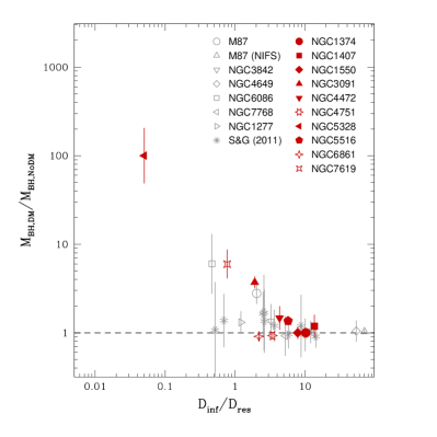
Figure 12: The ratio of $M_{\rm BH}$ from models with and without DM, versus relative spatial resolution. ${\rm D_{inf}}$ is the diameter of the sphere of influence of the black hole before taking into account DM and using the central $\sigma$ from HyperLeda. ${\rm D_{res}}$ is the diameter of the resolution element (see text). We include galaxies outside our sample for comparison purposes (M87, NGC 3842, NGC 4649, NGC 6086, NGC 7768, NGC 1277 and the sample of Schulze & Gebhardt 2011). There are two datapoints for M87, corresponding to the two measurements by Gebhardt & Thomas (2009) and Gebhardt et al. (2011) (marked as ’M87 (NIFS)’).

7.2 The influence of $\Upsilon$

Nine of the ten galaxies see a nominal change in $\Upsilon$ (Table 3). In all galaxies but NGC 6861 it systematically decreases from models without DM to models with DM. We show how the change in $\Upsilon$ is related to the change in $M_{\rm BH}$ in Fig. 13. We again include galaxies outside our sample for comparison.

The figure shows that the effect of DM on $M_{\rm BH}$ measurements is indirect, mediated by the $\Upsilon$. In galaxies where models with or without DM result in the same $\Upsilon$, the black-hole masses $M_{\rm BH}$ with DM and without DM are similar. The DM halo has no direct influence on the measured $M_{\rm BH}$. In most galaxies, however, the inclusion of DM leads to a reduction of the $\Upsilon$. Significant differences between $M_{\rm BH}$ determined with and without DM appear only in galaxies where the $\Upsilon$ changes significantly. Despite the different modelling approaches this behaviour is seen in all galaxies that have been analysed for DM so far.

The scatter in Fig. 13 is large. As already discussed above (Section 7.1) one source of scatter is the varying data resolution in the centre. In some galaxies the resolution is so good that despite a strong change in $\Upsilon$, $M_{\rm BH}$ stays constant because its determination is decoupled from $\Upsilon$. However, with decreasing resolution, $M_{\rm BH}$ and $\Upsilon$ become more and more degenerate. If the total central mass, i.e. the sum of $M_{\rm BH}$ and the stellar mass inside some small radius, would be entirely constrained by the observed kinematics, independently of whether DM is included in the outer parts or not, then the changes in $M_{\rm BH}$ and $\Upsilon$ should compensate for each other.

In Fig. 14 we test explicitly for this degeneracy by comparing the total enclosed mass of the best-fit model with DM and the best-fit model without DM, inside the same radius. As a benchmark we take $D_{\rm inf,DM}$ (calculated from the best-fit $M_{\rm BH}$ with DM). Comparison with Fig. 13 shows that the total mass in the centre is indeed better conserved than the masses of the stars and the BH individually. In most galaxies it is conserved to about $\sim 10$ percent, implying that the change in $M_{\rm BH}$ almost exactly compensates the change in the central stellar mass. When the $\chi^{2}$ changes drastically after the inclusion of dark matter (e.g. in NGC 5328), the central mass is not conserved, however. The $\Delta\chi^{2}$ between the corresponding models is sometimes over $\sim 1000$. Consequently, the fit without DM does not represent the data well and not even its total central mass is reliable. When this happens, the changes in $M_{\rm BH}$ and $\Upsilon$ from models without DM to models with DM are no longer mutually related to each other and can not be predicted. In fact, in some of our galaxies the change in $M_{\rm BH}$ overcompensates the change in $\Upsilon$ and the total mass in the centre increases. In addition to the varying data resolution, this adds to the scatter in Fig. 13 as well.

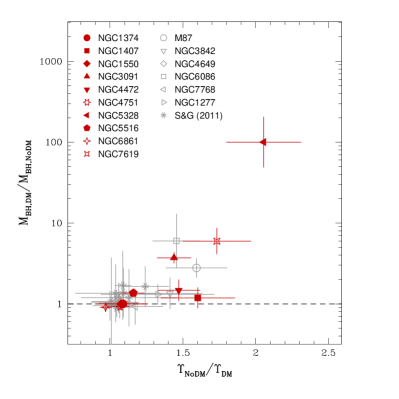
Figure 13: The ratio of $M_{\rm BH}$ with and without DM against the corresponding ratio for $\Upsilon$. Note the different numerator and denominator in both ratios. Galaxies outside our sample are included for comparison purposes and shown in grey (M87, NGC 3842, NGC 4649, NGC 6086, NGC 7768, NGC 1277 and the galaxies from Schulze & Gebhardt 2011).

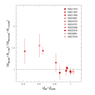
Figure 14: The relative change of the total mass (BH plus stars) inside the sphere of influence ${\rm D_{inf,DM}}$ of the best-fit BH (with DM) against the change in $\chi^{2}$.

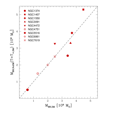
Figure 15: Comparison of the best-fit $M_{\rm BH}$ with DM (x-axis) and the best-fit $M_{\rm BH}$ one would get without DM in the models, but still using the correct (DM-based) mass-to-light ratio (y-axis; $\Upsilon\equiv\Upsilon_{\ast,\mathrm{DM}}$). NGC 5328 has been omitted because $\Upsilon_{\ast,\mathrm{DM}}$ is outside the grid of $\Upsilon$ probed without DM.

7.3 Modelling strategies

Our findings have straightforward implications for the modelling. As long as the sphere of influence is well sampled by the data, a biased $\Upsilon$ is not a problem in recovering the correct $M_{\rm BH}$ because $\Upsilon$ and $M_{\rm BH}$ are decoupled and, thus, including DM is not a necessity. The example for this would be NGC 1407. When the data resolution is not sufficiently high, it is important to have an unbiased $\Upsilon$ to derive an accurate $M_{\rm BH}$, as in the case of NGC 3091, NGC 5328 and NGC 7619.

Based on our results in Section 5.1, it is clear that including the DM is necessary to derive an unbiased dynamical $\Upsilon$. When DM is not included, the $\Upsilon$ obtained with less extended kinematic data is more reliable, although this does not completely remove the bias. It is however not clear, in advance of the modeling, where to spatially truncate the kinematic data. $R_{e}$ is not necessarily a good criterion. In the case of NGC 1407 and NGC 4472, the data go out to only a fraction of $R_{e}$ (around 0.5 and 0.25 $R_{e}$ respectively) but still contribute to an appreciable change in $\Upsilon$, while in NGC 1550 the change in $\Upsilon$ is within the error although the data extend out to $R_{e}$ (Table 3).

In Fig. 15 we compare the best-fit $M_{\rm BH}$ with DM to the best-fit $M_{\rm BH}$ that we get without DM, when we constrain $\Upsilon$ to its “correct” value (i.e. the value obtained from models with DM). Since the average ratio of these two $M_{\rm BH}$ determinations is $1.03$ with an rms-scatter of only $0.17$, one could recover $M_{\rm BH}$ accurately without DM if the correct $\Upsilon$ was known.

One could perhaps rely on the mass-to-light ratio derived from a single stellar population analysis ($\Upsilon_{\rm SSP}$). However, a major uncertainty in this approach is our ignorance related to the stellar IMF. Recent dynamical and lensing studies of early-type galaxies show that the amount of mass following the light differs from the prediction of SSP stellar masses based on a constant IMF. Galaxies with velocity dispersions around 200 km s^-1 are consistent with a Kroupa or Milky-Way like IMF, while at dispersions of 300 km s^-1 dynamical masses are a factor of 1.6-2.0 times larger than predicted by the same IMF (Cappellari et al. 2006; Napolitano, Romanowsky, & Tortora 2010; Treu et al. 2010; Thomas, Saglia, Bender et al. 2011; Cappellari, McDermid, Alatalo et al. 2012; Wegner, Corsini, Thomas et al. 2012). The interpretation of this trend as a systematic variation of the IMF with velocity dispersion depends on assumptions about the dark matter distribution. Independent support comes from the recent stellar-population models of near-infrared spectra by Conroy & van Dokkum (2012), which can reproduce the trend with velocity dispersion in terms of a variable stellar IMF.

At least two galaxies in our sample do not follow this trend, however. For NGC 1407, Spolaor et al. (2008b) give a central age of $12.0\pm 1.1$ Gyr and a metallicity of $0.29\pm 0.08$. Using the SSP models of Maraston (2005) and the galaxy’s velocity dispersion ($\sigma=276$ km s^-1) to estimate the IMF, we derive a stellar-population $\Upsilon_{\rm SSP}$ $=12.5\pm 3\,M_{\odot}/L_{\odot}$. Our dynamical models with DM yield instead a much lower value, $\Upsilon$ $=5.8-7.5\,M_{\odot}/L_{\odot}$. For NGC 7619, using the SSP analysis of Pu, Saglia, Fabricius et al. (2010) and estimating again the IMF from the galaxy’s velocity dispersion ($\sigma=292$ km s^-1), we get $\Upsilon_{\rm SSP}$ $=5.9\pm 1\,M_{\odot}/L_{\odot}$. As in NGC 1407, this is much larger than the dynamical $\Upsilon$ $=2.6-3.3\,M_{\odot}/L_{\odot}$. A similar result was found by van den Bosch et al. (2012) when modelling the BH, stars and dark matter in NGC 1277 simultaneously. Checks on a much larger sample of galaxies would be necessary to justify the use of $\Upsilon_{\rm SSP}$ as a surrogate.

8 Black hole-bulge relation

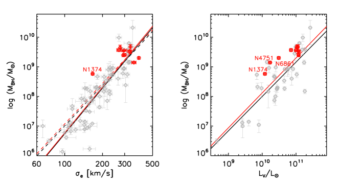
Figure 16: The $M_{\rm BH}$-$\sigma$ (left) and ${M_{\rm BH}}$-$L$ (right) diagrams with our updated relations. Grey diamonds are the galaxies in the sample of McConnell et al. (2011b). The relations that they derive are indicated by black lines. The solid and dashed black lines in the $M_{\rm BH}$-$\sigma$ relation show the fit to all galaxies and to only the early-type galaxies in their sample, respectively. The red diamonds represent the ten galaxies in our sample, where we plot $M_{\rm BH}$ obtained by taking into account the DM. Using the McConnell et al. sample and these ten galaxies, we updated the relations, shown by the red lines. The solid and dashed red lines in the $M_{\rm BH}$-$\sigma$ relation use the ’all1’ and ’early-type’ sample, respectively (see Table 4).

We consider the latest version of the $M_{\rm BH}$-$\sigma$ and ${M_{\rm BH}}$-$L$ relations derived by McConnell et al. (2011b) in Fig. 16. We do not consider the results of McConnell & Ma (2013), because they are based on a sample that lists preliminary values of a subset of the galaxies analysed here. The galaxies in the sample of McConnell et al. (2011b) are plotted in grey and their relations are shown by the black lines. In the $M_{\rm BH}$-$\sigma$ diagram, the solid and dashed lines are the fit to all galaxies in the sample and to only early-type galaxies, respectively. We overplot our new measurements as red diamonds; we calculate the velocity dispersion of the ten galaxies as in Gültekin et al. (2009), i.e. $\sigma_{e}^{2}=\int_{0}^{R_{e}}{(\sigma^{2}+V^{2})I(r)dr/\int_{0}^{R_{e}}{I(r)dr}}$ and the $M_{\rm BH}$ values are the ones obtained with DM. All galaxies lie well above the ${M_{\rm BH}}$-$L$ relation of McConnell et al. (2011b). In the $M_{\rm BH}$-$\sigma$ diagram, two galaxies (NGC 6861 and NGC 4751) fall below their relation.

The standard parametrization of the $M_{\rm BH}$-$\sigma$ and ${M_{\rm BH}}$-$L$ relationships are ${\rm log_{10}}(M_{\rm BH}/M_{\odot})=\alpha+\beta\,{\rm log_{10}}(\sigma/200\,{\rm km~{}s}^{-1})$ and ${\rm log_{10}}(M_{\rm BH}/M_{\odot})=\alpha+\beta\,{\rm log_{10}}(L_{V}/10^{11}L_{\odot})$, respectively, with some intrinsic scatter $\epsilon_{0}$. This functional form is a single-index power law with $\alpha$ as the zero-point and $\beta$ as the slope. We refitted the relationships after incorporating our black hole measurements by using a Bayesian method with Gaussian errors and intrinsic scatter $\epsilon_{0}$ as described in Kelly (2007), assuming that the uncertainties in the luminosities or velocity dispersions are not correlated with those in the black hole masses. We were able to recover the $M_{\rm BH}$-$\sigma$ and ${M_{\rm BH}}$-$L$ relations and their intrinsic scatters as fitted by Gültekin et al. (2009) and McConnell et al. (2011b), using their corresponding samples. For our new fits, we define three samples: The sample “all1” refers to all galaxies in the sample of McConnell et al. (2011b) plus our ten galaxies. The “early-type” sample is the early-type subset of “all1”. ”all2” contains the “ML” sample of McConnell et al. (2011b) plus the ten galaxies from this work. The fit results are given in Table 4 for each relationship and shown in Fig. 16 as red lines. In the ${M_{\rm BH}}$-$L$ fit we adopt an uncertainty for each $M_{V}$ of 0.1 magnitude, compatible with the extrapolation errors in our integrated luminosity profiles. Note that the fit parameters and the intrinsic scatter are not very sensitive to a precise ${\rm M_{V}}$ uncertainty. Collectively, our ten galaxies introduce a negligible change in the $M_{\rm BH}$-$\sigma$ relation of McConnell et al. (2011b) and a slight increase in the zeropoint of their ${M_{\rm BH}}$-$L$ relation, such that a given luminosity now corresponds to a higher $M_{\rm BH}$.

The average deviation of our galaxies from the new $M_{\rm BH}$-$\sigma$ relation is 0.47 dex in $M_{\rm BH}$ for the “all1” sample and 0.42 dex for the early-type sample. Our galaxies are located 0.43 dex away from the derived ${M_{\rm BH}}$-$L$ relation, on average. If we use the relations of McConnell et al., then the average deviation would be higher, i.e. 0.48, 0.44 and 0.53 dex from the $M_{\rm BH}$-$\sigma$ (all), $M_{\rm BH}$-$\sigma$ (early-type) and the ${M_{\rm BH}}$-$L$ relations, respectively. The above mean deviations are equal to the intrinsic scatter in the respective relations, except for our ${M_{\rm BH}}$-$L$ relation, which has a larger intrinsic scatter.

The galaxy that is farthest from the $M_{\rm BH}$-$\sigma$ relation is NGC 1374, for which we do not see a change in $M_{\rm BH}$ due to DM. If NGC 1374 is intrinsically flattened and seen close to face-on, then we have observed the smallest projected velocity dispersion possible. NGC 4751 deviates the most in the ${M_{\rm BH}}$-$L$ relation: the galaxy luminosity is approximately a factor 4 too small for its black hole mass.

Table 4: Parametric fits for the $M_{\rm BH}$-$\sigma$ and ${M_{\rm BH}}$-$L$ relations

Diagram	Sample	$\alpha$	$\beta$	$\epsilon_{0}$
$M_{\rm BH}$-$\sigma$	all1	$8.32\pm 0.05$	$5.16\pm 0.32$	0.44
$M_{\rm BH}$-$\sigma$	early-type	$8.44\pm 0.06$	$4.55\pm 0.34$	0.39
${M_{\rm BH}}$-$L$	all2	$9.30\pm 0.10$	$1.18\pm 0.13$	0.50

Based on the black hole-bulge relationships, combined with a velocity dispersion or luminosity function, one can construct an estimate of the local black hole space density. Lauer et al. (2007a) and Gültekin et al. (2009) find a marked discrepancy between the $L$-based and $\sigma$-based local density of the largest black holes ($M_{\rm BH}\gtrsim 10^{9}$$M_{\odot}$), i.e. the former is significantly larger than the latter. Using our results from Table 4, we derive the cumulative density distribution of black holes (see Fig. 17) following the same approach and assumptions as in Lauer et al. (2007a), which were also used by Gültekin et al. (2009). The dispersion-based density is computed using the velocity dispersion function of Sheth et al. (2003) in the form of Schechter function fit. To this, a correction to the number of high-$\sigma$ galaxies ($\sigma>350$ km s^-1) is applied based on the work of Bernardi et al. (2006). For the L-based space density, we use the SDSS g’ luminosity function of Blanton, Hogg, Bahcall et al. (2003), converted to the V-band. The high-L part of this function is corrected by adding an estimate of the BCG luminosity function of Postman & Lauer (1995). We refer the reader to Section 6.1 of Lauer et al. (2007a) for a more thorough description.

The $M_{\rm BH}$-$\sigma$ relation fitted here has a considerably higher zeropoint, slope and intrinsic scatter than those derived in Gültekin et al. (2009), leading to a higher $\sigma$-based BH density which should therefore place the latter closer to the prediction based on the ${M_{\rm BH}}$-$L$ relation. However, the intrinsic scatter and the zeropoint in our ${M_{\rm BH}}$-$L$ fit are also larger compared to those in Gültekin et al. (2009), which results in an even higher luminosity-based BH density. Since 2009, a number of $M_{\rm BH}$ measurements have been added to the high-$M_{\rm BH}$ part of the relationships, which have changed the correlations quite significantly. As shown in Fig. 17, the difference between the two mass functions is not reconciled using our updated $M_{\rm BH}$-$\sigma$ and ${M_{\rm BH}}$-$L$ relations. Black holes more massive than $10^{9}$ $M_{\odot}$ now correspond to $\sigma\gtrsim 280$ km s^-1 or $L_{\rm V}\gtrsim 7\times 10^{10}L_{\odot}$ (Fig. 16) and there are fewer galaxies with $\sigma>280$ km s^-1 than there are galaxies with $L>7\times 10^{10}L_{\odot}$. If the ${M_{\rm BH}}$-$L$ relation were to have the same scatter as the $M_{\rm BH}$-$\sigma$ relation, the predicted space density of BH for the largest BHs would be in a better agreement: a lower intrinsic scatter results in fewer high-mass black holes (see Fig. 3 of Lauer, Tremaine, Richstone et al. 2007b).

Lauer et al. (2007a) make a comparison between the local BH cumulative space density estimated from the BH–host-galaxy relations and the density estimated from luminous QSOs; they argue that this comparison favors the the ${M_{\rm BH}}$-$L$ relation, since the $M_{\rm BH}$-$\sigma$ relation seems to underpredict the density of the most massive BHs compared to the QSO-based models (their Fig. 11). In contrast to their results, we find that the updated ${M_{\rm BH}}$-$L$ and $M_{\rm BH}$-$\sigma$ relations both overpredict the density of the most massive BHs compared to the same QSO models (Fig. 17). Since the ${M_{\rm BH}}$-$L$ relation predicts the highest density of BHs at the upper-mass end, it is now the prediction from the $M_{\rm BH}$-$\sigma$ relation which is the better match to the same QSO models (represented by the “Hopkins” and “lightbulb” lines in Fig. 17) is now that from the $M_{\rm BH}$-$\sigma$ relation. Nonetheless, even this relation appears to predict a BH density about an order of magnitude larger than that from the QSO models for $M_{\rm BH}\gtrsim 10^{9}$ $M_{\odot}$. We note, however, that there is considerable uncertainty and freedom in QSO-based models of BH space density, depending on factors such as how Eddington vs. sub-Eddington accretion duty cycles are handled, overall radiative efficiency, etc. (see, e.g., Kelly & Merloni, 2012).

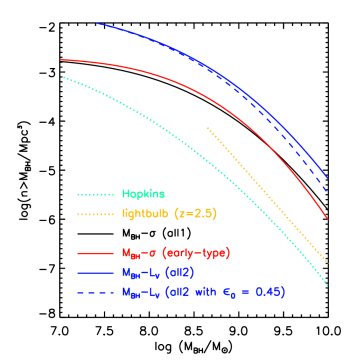
Figure 17: Black hole cumulative space density derived from the $M_{\rm BH}$-$\sigma$ and ${M_{\rm BH}}$-$L$ relations in Table 4 (solid lines). If the intrinsic scatter of the ${M_{\rm BH}}$-$L$ relation is the same as that of the $M_{\rm BH}$-$\sigma$ relation (all1 sample), the resulting space density is shown by the dashed blue line. The lightbulb model is based on the luminosity function from SDSS at a redshift of z=2.5 (Richards, Croom, Anderson et al., 2005) and the Hopkins model is based on the quasar model of Hopkins, Hernquist, Cox et al. (2006). Both quasar models are identical to those in Fig. 11 of Lauer et al. (2007a)

9 Summary

This paper presents new AO-assisted SINFONI observations of ten nearby early-type galaxies, nine of which have velocity dispersions greater than 250 km s^-1. The SINFONI data are complemented by other ground-based data with larger spatial scales, which are found in the literature or come from new observations. We use the data to measure the masses $M_{\rm BH}$ of supermassive black holes in the centers of these galaxies using three-integral axisymmetric orbit-superposition models. The black hole masses reported here represent the first such dynamical measurements for each of the sample galaxies.

We pay particular attention to the question of how including or ignoring a dark matter (DM) halo in the dynamical models affects the derived $M_{\rm BH}$. We adopt a cored logarithmic profile for the DM halo. For seven galaxies, where the kinematic data extend to large radii, the parameters of the halo are determined by the fitting process; for the others, we set the halo parameters to fixed values based on the $L_{B}$–DM scaling relation of Thomas, Saglia, Bender et al. (2009).

We first study models without black holes; this shows that omitting DM in the modeling results in a bias in the stellar M/L ratio $\Upsilon$, which is systematically higher when DM is not included. This bias becomes stronger when the spatial extent of the kinematic data is maximised. This suggests that it is necessary to consider DM in the dynamical modeling in order to derive a reliable value of $\Upsilon$.

We then explore models with and without DM which include black holes, and we assess how changes in $\Upsilon$ or data resolution affect the black hole mass determination. For completeness, we include $M_{\rm BH}$ measurements, with and without DM, for 17 massive galaxies from the literature. We find that changes in $M_{\rm BH}$ are triggered by changes in $\Upsilon$ due to DM inclusion. The underlying relationship between $M_{\rm BH}$ and the DM halo is indirect: including the DM halo affects $\Upsilon$, which in turn affects $M_{\rm BH}$. If we fix $\Upsilon$ to the “correct” value (i.e., that obtained by including DM in the modeling), then the “correct” value of $M_{\rm BH}$ is obtained from the modeling even if DM is excluded.

The ratio between the black hole mass determined with a DM halo model and the mass determined without one, $M_{\rm BH,DM}/M_{\rm BH,NoDM}$, shows scatter and bias which increases as the spatial resolution of the central kinematic data decreases. If we define the resolution relative to the BH’s sphere of influence as $D_{\rm inf}/D_{\rm res}$, where $D_{\rm inf}$ is the size of the sphere of influence (using $M_{\rm BH}$ from models without DM) and $D_{\rm res}$ is the best resolution of the observations, then $M_{\rm BH}$ is significantly underestimated for $D_{\rm inf}/D_{\rm res}<5$ when DM is not included. For $D_{\rm inf}/D_{\rm res}>10$, $M_{\rm BH}$ is negligibly affected by the presence or absence of DM, despite the large change in $\Upsilon$; $M_{\rm BH}$ and $\Upsilon$ are effectively decoupled when the resolution is this good. For values of $D_{\rm inf}/D_{\rm res}$ between 5 and 10, $M_{\rm BH}$ can be underestimated by about 30 percent if DM is not included, a level similar to typical measurement errors for $M_{\rm BH}$.

All of the measured BH masses are located above the ${M_{\rm BH}}$-$L$ relation of McConnell et al. (2011b); seven of the ten galaxies have BH masses above their $M_{\rm BH}$-$\sigma$ relation. Including these ten galaxies in the relationships introduces a negligible change in the $M_{\rm BH}$-$\sigma$ relation and slightly increases the zeropoint of the ${M_{\rm BH}}$-$L$ relation, such that a given luminosity now corresponds to a higher $M_{\rm BH}$. Using our updated relations, we find that the cumulative space density of the most massive black holes predicted by the ${M_{\rm BH}}$-$L$ relation is about one order of magnitude higher than that predicted by the $M_{\rm BH}$-$\sigma$ relation. The latter predictions, in turn, are about an order of magnitude higher than the quasar-count-based density models from Lauer et al. (2007a), which inverts the claim made in that study (that the $M_{\rm BH}$-$\sigma$ relation predicts too few high-mass black holes to match the quasar-count models).

Appendix A The long-slit kinematics of NGC 1374 and NGC 6861

The long-slit observations of NGC 1374 and NGC 6861 were part of the program described by Saglia, Maraston, Thomas et al. (2002). NGC 1374 was observed during the period 2001 November 10–14 at the La Silla ESO NTT telescope, equipped with the EMMI spectrograph. We used the red arm (REMD mode with longslit, 6 arcmin long) with the 13.5  Å mm^-1 grating (#6), the OG530 order sorting filter and the Tektronix $2048\times 2047$ 24-$\mu$m pixels CCD. The slit width was 3″ and the scale 0.27 arcsec/pixel, giving a resolution of 70 km s^-1 and covering the wavelength range $\lambda=8298-8893$Å. We observed the galaxy at PA=120 with 90 minutes integration time.

NGC 6861 was observed during the period 2001 May 8–14 at the 2.3 Siding Spring telescope, where we used the red arm of the Double Beam Spectrograph (Rodgers et al., 1988) in longslit (6.7 arcmin) mode with the 600 R grating (73  Å mm^-1) grating, no beamsplitter and the Site $1752\times 532$ 15-$\mu$m pixels CCD. The slit width was 3.5″ and the scale was 0.91 arcsec/pixel, giving a resolution of 75 km s^-1 and covering the wavelength range $\lambda=7645-9573$. We observed the galaxy at PA=142 with 142 min integration time.

The standard CCD data reduction was carried out with the image processing package MIDAS provided by ESO. After bias subtraction and flatfielding, the fringing disappeared, resulting in CCD spectra flat to better than 0.5% and slit illumination uniform to better than 1%. No correction for dark current was applied, since it was always negligible. Hot pixels and cosmic ray events were removed with a $\kappa-\sigma$-clipping procedure. The wavelength calibration was performed using calibration lamps (HeAr, FeNe, FeAr) for NGC 6861, and sky lines for NGC 1374, where the calibration lamp exposures were too weak or not enough calibration lines were present in the wavelength range. A third order polynomial was used to perform the calibration, achieving 0.1 Å rms precision. The spectra were rebinned to a logarithmic wavelength scale and the mean sky spectrum during each exposure was derived by averaging several lines from the edges of the CCD spectra. By applying the same procedure to the blank sky observations, the systematic sky residuals were measured to be less than 1%. After subtraction of the sky spectra, spectra of the same galaxy taken at identical slit positions were centred and added; one-dimensional spectra were produced for the kinematic standard stars. The galaxy spectra were rebinned along the slit in order to guarantee a signal-to-noise ratio that allowed the derivation of the kinematic parameters.

The galaxy kinematics were derived using the Fourier Correlation Quotient (FCQ) method (Bender 1990). Following Bender, Saglia and Gerhard (1994, hereafter BSG94), the line-of-sight velocity distributions (LOSVDs) were measured and fitted to provide the stellar rotational velocities $V$, the velocity dispersions $\sigma$ and the first orders of asymmetric ($h_{3}$) and symmetric ($h_{4}$) deviations of the LOSVDs from real Gaussian profiles. Monte Carlo simulations were performed to establish that a fourth order polynomial in the wavelength range $\approx 8250-8950$Å provided good continuum fits, resulting in systematic residuals always smaller than the estimated statistical errors. These were calibrated testing a grid of input S/N, taking into account the noise contributions of the galaxy and the sky signals. The errors from systematics in the sky subtraction (at the 1% level, see above) were less than the statistical errors. Tables 5 and 6 give the resulting kinematics.

Table 5: The long-slit kinematics of NGC 1374

R (″)	V (km s-1)	dV (km s-1)	$\sigma$ (km s-1)	$d\sigma$ (km s-1)	$h_{3}$	$dh_{3}$	$h_{4}$	$dh_{4}$
-15.16	-46.18	9.42	106.82	14.21	-0.087	0.069	0.045	0.067
-4.62	-50.65	3.14	134.27	4.11	-0.090	0.024	0.042	0.028
-1.76	-51.9	2.00	144.72	2.28	-0.003	0.010	0.001	0.016
-0.63	-28.74	2.23	171.29	3.00	-0.025	0.012	0.015	0.014
0.14	10	2.15	180.22	2.92	0.013	0.011	-0.013	0.009
1.04	40.45	1.95	168.26	3.22	0.041	0.012	0.016	0.012
2.66	49.13	2.49	146.97	2.89	0.054	0.012	0.033	0.017
7.29	42.56	2.70	139.42	3.63	0.050	0.027	-0.012	0.023
19.83	46.67	11.75	118.26	11.72	-0.036	0.121	-0.065	0.090

Table 6: The long-slit kinematics of NGC 6861

R (″)	V (km s-1)	dV (km s-1)	$\sigma$ (km s-1)	$d\sigma$ (km s-1)	$h_{3}$	$dh_{3}$	$h_{4}$	$dh_{4}$
-10.01	-257.90	13.73	279.18	11.94	0.195	0.033	-0.107	0.039
-7.78	-273.20	9.91	275.60	8.89	0.201	0.025	-0.107	0.029
-5.96	-263.80	9.36	299.99	10.24	0.173	0.021	-0.029	0.026
-4.14	-235.30	7.84	307.07	12.17	0.128	0.022	0.001	0.026
-2.81	-196.60	10.48	323.65	13.82	0.116	0.022	0.067	0.032
-1.90	-126.20	8.38	362.01	8.09	0.139	0.022	0.050	0.021
-0.99	-81.17	8.37	365.61	6.58	0.065	0.017	0.050	0.021
-0.08	0.89	9.07	403.95	11.68	0.083	0.016	0.034	0.021
0.84	70.00	10.72	380.21	10.71	0.019	0.018	-0.015	0.022
1.75	128.90	7.97	361.96	10.57	-0.012	0.017	0.019	0.024
2.66	196.60	8.82	333.02	7.74	-0.065	0.020	-0.031	0.022
3.57	258.80	9.17	311.83	9.65	-0.092	0.017	0.044	0.032
4.89	273.30	8.16	299.81	10.54	-0.084	0.020	-0.003	0.025
6.72	284.70	10.21	275.83	11.75	-0.100	0.029	-0.040	0.036
8.94	260.80	12.40	292.37	15.25	-0.046	0.035	-0.043	0.040

Appendix B The VIRUS-W kinematics of NGC 3091 and NGC 5328

The observations of NGC 3091 and NGC 5328 were carried out using the new VIRUS-W spectrograph (Fabricius, Grupp, Bender et al., 2012) at the 2.7 m Harlan J. Smith telescope at the McDonald Observatory in Texas. NGC 3091 was observed during the commissioning of VIRUS-W in December 2010 while for NGC 5328 we were granted with two nights of observing time in May 2011.

VIRUS-W offers a fiber-based Integral Field Unit (IFU) with a field of view (FoV) of 105 arcsec$\times$55 arcsec. The 267 individual fibers have a core diameter of 3.14 arcsec on sky. The fibers are arranged in a rectangular matrix in a densepack scheme with a fill factor of 1/3, such that three dithered observations are necessary in order to achieve 100 % coverage of the FoV. The instrument offers further two different modes of spectral resolution. For both galaxies we used the lower resolution mode (R = 3300, translating to $\sigma_{instr}=39$ km s^-1) with a spectral coverage of 4320 Å to 6042 Å.

We obtained dithered observations of two off-centred and slightly overlapping regions of NGC 3091 and NGC 5328 in the night of December 5 and the two nights of May 24 and 25 respectively. The two plots in Fig. 18 show images of the two galaxies with boxes that outline the field positions.

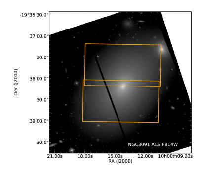
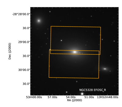
Figure 18: Left panel: HST ACS F814W image of NGC 3091. The boxes outline the instrumental FoV of our two different VIRUS-W fields. Right panel: VIRUS-W FoV for NGC 5328 overplotted on a EFOSC2 R band (Grützbauch et al., 2005) image.

The exposure time of the individual on-object pointings was 600 s for NGC 3091 and 700 s for NGC 5328. We repeated each pointing once for cosmic ray rejection, resulting in a total on-object integration time of 2 h and 2.3 h for NGC 3091 and NGC 5328 respectively. All on-object observations were bracketed and interleaved with 300 s sky nods that were offset by 9 arcmin to the north. During the observations of NGC 3091 the seeing varied from 2.0 to 2.2 arcsec (FWHM) while for NGC 5328 it varied from 2.0 to 2.5 arcsec, which is small compared to the fiber size. In addition to the galaxies, we also observed the two giant stars HR 7576 and HR 2600 which serve as templates for the kinematic extraction.

We extracted the individual fiber spectra using the cure pipeline that was originally developed by Ralf Koehler, Niv Drory and Jan Snigula for the HETDEX experiment. The basic image reduction uses the fitstools package (Gössl & Riffeser, 2002) and follows standard recipes for creation and subtraction of master bias frames and the averaging of flat fields and calibration lamp frames. cure traces the positions of the fiber spectra on the chip using the twilight or dome flat frames and then searches for the calibration lamp line positions along those traces. Trace and wavelength positions are modelled as a two-dimensional Chebyshev polynomial of 7-th degree across the CCD surface. The standard deviation of this wavelength/distortion solution is 0.2  pixels which corresponds to 0.1 Å at the linear dispersion of 0.52 Å/pixel. In the next step, cure calculates transformations between fiber number/wavelength and x/y positions and corresponding inverse and cross transformations. Given these models for fiber position and wavelength calibration, the fiber extraction walks along the trace positions across the CCD and extracts the spectra at given wavelength steps. We used a 7-pixel-wide extraction aperture around the centroid position of the individual fiber spectra. Tests showed that this results in less than 1 % loss of flux and less than 0.1 % crosstalk between neighbouring spectra.

The extraction produces a total of $2\times 3\times 267=1062$ wavelength calibrated spectra, corresponding to the two fields with three dithers and 267 fiber apertures. We extracted spectra binned linearly in wavelength space.

Preliminary kinematic maps for NGC 3091 showed unrealistic north-south gradients of the dispersion which we identified to be a consequence of an imperfect sky subtraction when the data of the interleaved sky nods were used. We rejected the data from the sky nods and identified fibers around the edges of the combined FoV to estimate the background. We selected them to be located further than 50 arcsec from the galaxy center and visually rejected fibers that fall on the neighbouring galaxy MCG -03-26-006. We averaged the skyfiber spectra for each dither position separately while rejecting spurious events using a standard, iterative kappa-sigma-clipping algorithm. The resulting average sky spectrum is subtracted from the corresponding object spectra.

For NGC 5328 the use of the sky nods did not result in similar gradients. We averaged the bracketing sky exposures for each science exposure while rejecting cosmics. The sky signal is then calculated from the extracted sky spectra by averaging the flux of 20 neighbouring fibers in a moving window approach. The resulting spectra are scaled by exposure time and subtracted from the science data.

The modelling employs a radial binning scheme for the SINFONI data described in Section 3. For NGC 3091 we binned the VIRUS-W data following the same procedure. The binning step again rejects residual events. Bins that are located inside a radius of 10 arcsec around the center are rejected because there the size of the fiber aperture is comparable or larger than the bin size of the radial binning scheme. The median S/N per Å in the final bins is 19.

For NGC 5328 we instead employed a Voronoi binning scheme. The bin sizes were calculated using the code of Cappellari & Copin (2003) and then combined in the same manner as for NGC 3091. The minimum S/N per Å in the used bins is 25 with a median of 40.

After rebinning of the spectra into log-wavelength space, we used the Fourier Correlation Quotient (FCQ) algorithm (FCQ; Bender, 1990; BSG94) to extract the line of sight velocity distributions. For this work, we use a single template spectrum of the K3III star HR 7576. We tested fits with the additional K2III star HR 2600, which yielded consistent results. We fit the kinematics in the rest frame spectral range from 4537 Å to 5443 Å. The continuum is removed using an 8th degree polynomial and the first and last three channels in the Fourier space are filtered out. We finally used Monte Carlo simulations as described in Mehlert, Saglia, Bender et al. (2000) for the derivation of statistical errors.

Table 7 provides the resulting kinematics for NGC 3091, using the same spatial binning scheme as for the SINFONI data shown in Fig. 2-5. Table 8 shows the kinematics for the folded quadrant used in the model. The velocities $V$ are given relative to the average velocity. Similarly, Table 9 gives the resulting kinematics for NGC 5328. The Voronoi bin centers are listed in the first two columns. The velocities $V$ are given relative to the average velocity.

Table 7: The VIRUS-W Kinematics of NGC 3091: four quadrants

Radius (″)	iv	$V$ (km s-1)	$dV$ (km s-1)	$\sigma$ (km s-1)	$d\sigma$ (km s-1)	$h_{3}$	$dh_{3}$	$h_{4}$	$dh_{4}$
-42.29	-3	-156.03	20.43	235.67	18.02	0.130	0.045	-0.059	0.032
-42.29	-1	-150.63	18.92	272.33	25.56	0.043	0.037	-0.008	0.031
-42.29	1	-207.45	15.69	221.72	21.44	0.004	0.044	-0.086	0.031
-42.29	3	-134.08	39.99	322.73	56.95	0.034	0.050	-0.034	0.053
-32.75	-5	-8.43	30.24	323.64	35.80	0.088	0.043	0.034	0.035

Table 8: The VIRUS-W Kinematics of NGC 3091: the folded quadrant

Radius (″)	iv	$V$ (km s-1)	$dV$ (km s-1)	$\sigma$ (km s-1)	$d\sigma$ (km s-1)	$h_{3}$	$dh_{3}$	$h_{4}$	$dh_{4}$
11.73	1	88.63	6.67	292.87	6.59	-0.016	0.016	-0.008	0.016
15.17	1	100.14	6.50	284.19	6.52	-0.020	0.016	-0.004	0.016
19.61	1	116.13	7.21	296.92	7.00	-0.020	0.017	-0.018	0.017
25.35	1	130.88	7.30	286.45	7.40	-0.022	0.018	-0.001	0.017
32.75	1	108.75	7.81	303.42	7.50	-0.015	0.018	-0.025	0.017
42.29	1	157.37	7.90	268.64	7.54	-0.015	0.020	-0.028	0.019
11.72	2	72.27	6.56	284.45	6.59	-0.002	0.016	-0.005	0.016
25.35	2	112.73	6.88	275.51	6.78	-0.013	0.018	-0.015	0.017
32.75	2	132.37	7.78	294.77	7.28	-0.032	0.018	-0.038	0.018
11.72	3	73.21	6.75	290.16	6.76	0.015	0.016	-0.002	0.016
15.17	3	50.97	6.88	290.66	6.82	-0.004	0.017	-0.010	0.016
19.61	3	78.73	6.89	298.15	6.24	-0.021	0.016	-0.045	0.016
25.35	3	95.69	6.94	283.83	6.49	-0.025	0.017	-0.034	0.017
32.75	3	110.00	8.17	303.03	7.88	0.004	0.019	-0.024	0.018
42.29	3	102.34	10.27	300.84	9.90	-0.022	0.023	-0.025	0.021
11.72	4	42.38	6.54	277.24	6.56	-0.007	0.016	-0.002	0.016
15.17	4	59.26	6.68	277.34	6.65	0.014	0.017	-0.004	0.017
19.61	4	58.89	7.12	311.81	6.55	-0.008	0.016	-0.039	0.016
25.35	4	73.76	7.53	291.71	7.63	-0.031	0.018	-0.001	0.018
32.75	4	69.99	7.97	280.78	8.15	-0.031	0.020	-0.007	0.019
11.72	5	23.11	6.38	278.03	6.71	0.019	0.016	0.019	0.016
15.17	5	20.00	6.23	266.46	6.15	0.001	0.016	-0.007	0.016
19.61	5	15.97	6.44	260.06	6.20	0.023	0.017	-0.017	0.017
25.35	5	22.20	6.86	263.70	6.68	0.007	0.018	-0.018	0.018
32.75	5	23.16	7.65	264.44	7.89	-0.031	0.020	0.005	0.019

Table 9: The VIRUS-W Kinematics of NGC 5328

x (″)	y (″)	$V$ (km s-1)	$dV$ (km s-1)	$\sigma$ (km s-1)	$d\sigma$ (km s-1)	$h_{3}$	$dh_{3}$	$h_{4}$	$dh_{4}$
0.14	1.44	11.86	5.45	365.91	5.64	-0.011	0.009	0.032	0.010
0.32	0.84	4.47	8.31	380.59	8.66	-0.039	0.013	0.020	0.017
0.27	3.98	-4.47	13.86	364.20	16.18	-0.027	0.023	0.045	0.023
2.53	3.20	-14.69	8.75	344.91	9.57	-0.020	0.014	0.025	0.016
-0.59	10.12	-7.79	6.76	319.64	9.62	-0.011	0.017	0.003	0.017
-0.20	4.55	14.76	11.47	347.10	13.51	-0.029	0.020	0.024	0.018
2.82	0.19	12.83	12.73	359.68	14.04	-0.023	0.019	0.012	0.023
3.25	-0.39	-3.25	14.54	348.74	16.36	-0.051	0.021	0.004	0.024
-2.41	2.23	1.93	13.92	367.98	13.59	0.006	0.018	0.001	0.020
-2.80	2.70	15.40	6.94	370.44	7.95	0.000	0.012	0.053	0.013
-2.54	-0.31	-1.29	8.47	369.81	11.09	-0.012	0.014	0.030	0.017
-2.10	-0.93	29.23	9.59	366.87	11.88	-0.015	0.019	0.020	0.018
0.58	-2.17	-18.73	10.68	333.10	12.94	0.001	0.022	0.004	0.023
-2.85	5.66	12.72	10.59	328.00	9.96	0.000	0.015	0.005	0.017
-5.07	15.42	16.40	7.16	298.97	10.68	0.014	0.015	0.035	0.019
3.35	8.70	-6.00	7.51	317.11	8.94	-0.013	0.015	0.015	0.015
7.12	19.26	-24.02	6.37	251.77	10.02	0.025	0.017	0.034	0.020
-5.12	3.51	13.76	12.76	351.44	15.83	0.017	0.023	0.016	0.023
-5.08	0.84	0.54	8.48	339.17	8.22	-0.001	0.013	0.014	0.014
-5.04	0.33	-19.94	10.50	355.19	12.10	-0.040	0.020	-0.011	0.019
-8.93	7.33	36.24	8.35	318.68	9.06	0.018	0.013	0.015	0.016
-5.56	4.08	8.15	12.29	357.87	12.71	-0.019	0.020	-0.006	0.018
-0.20	-9.84	5.40	5.84	280.98	9.85	-0.020	0.016	0.025	0.016
-1.86	-3.47	16.22	9.84	346.22	12.14	0.040	0.018	0.040	0.016
-4.81	-2.22	28.34	10.29	346.75	11.43	0.042	0.017	0.003	0.022
-5.82	-7.84	36.81	9.65	301.21	11.98	0.011	0.018	0.026	0.020
-0.58	-20.40	0.50	6.38	270.63	8.52	-0.052	0.015	0.034	0.016
-7.94	1.98	4.90	8.04	303.80	9.52	0.010	0.016	0.011	0.017
-19.08	7.40	70.12	6.99	278.10	7.54	-0.005	0.015	-0.019	0.015
-12.81	1.48	59.15	5.67	298.24	8.20	0.030	0.013	0.016	0.012
-13.78	19.79	45.78	10.24	299.89	12.51	0.005	0.020	0.004	0.021
-9.10	-5.04	53.46	9.79	313.76	9.75	0.010	0.017	0.000	0.015
-16.18	-6.96	78.87	8.42	302.84	9.32	0.030	0.014	0.009	0.016
-7.61	-1.11	20.66	10.91	345.02	11.26	-0.022	0.020	0.004	0.020
-27.52	-4.08	117.83	7.54	283.45	9.55	0.065	0.019	-0.005	0.017
-12.11	-18.81	39.38	6.42	287.55	7.50	-0.017	0.016	0.004	0.015
7.42	7.45	-37.88	8.37	304.66	10.30	-0.012	0.018	0.006	0.018
16.96	12.47	-67.12	6.60	280.65	8.00	-0.013	0.017	-0.032	0.014
5.56	1.77	-12.65	9.24	334.85	13.65	-0.035	0.018	0.035	0.018
10.80	2.82	-36.74	8.02	306.04	8.68	-0.032	0.016	0.012	0.015
4.85	-5.29	-16.55	7.99	347.65	9.91	-0.019	0.014	0.042	0.014
9.07	-15.65	-24.16	6.16	271.87	7.25	0.000	0.015	0.000	0.014
11.62	-5.40	-44.78	8.04	299.28	9.48	-0.040	0.020	0.027	0.018
5.67	-1.31	-8.51	9.38	341.20	9.63	-0.020	0.016	0.006	0.017
21.69	-1.25	-81.45	6.42	251.71	6.31	-0.027	0.014	-0.041	0.015
20.24	-16.77	-51.68	6.68	277.99	7.65	-0.007	0.015	-0.025	0.014

Appendix C The WiFeS Kinematics of NGC 4751 and NGC 5516

NGC 4751 and NGC 5516 were observed in May 2010 at the ANU 2.3m telescope at Siding Spring Observatory. The instrument was WiFeS Integral Field spectrograph (Dopita, Hart, McGregor et al., 2007; Dopita, Rhee, Farage et al., 2010). The dual-beam system was used with the B3000 and R7000 VPH grating combination with Dichroic $\#$3. For NGC 4751 we collected 6x1200 sec exposures in May 2010 and a 1200 sec sky exposure. For NGC 5516 3x1200 sec object exposures plus a 1200 sec sky exposure were taken on 2010 May 19. The data reduction was performed using the dedicated IRAF pipeline software of the instrument. We derived the stellar kinematics from the blue frames, focusing on the wavelength region $\lambda=4900-5400$Å, where we achieved a spectroscopic resolution of $\sigma_{\rm inst}=58$ km s^-1 measured from the width of the sky lines. The stellar kinematics was measured with the software described in Saglia, Fabricius, Bender et al. (2010) and Fabricius, Saglia, Fisher et al. (2012). This uses the FCQ method of BSG94 in combination with a stellar library convolved to the instrumental resolution and can be applied iteratively to detect and subtract possible emission lines. However, no detectable emission was found. Table 10 and 11 give the resulting kinematics for NGC 4751 and NGC 5516. We give the kinematics along NS slits (with positive radii indicating distances in arcsec from the center of the galaxy towards the North and negative radii towards the South), shifted with respect to the center of the galaxy along the East (positive shifts in arcsec) or West (negative shifts) directions. The velocities of NGC 4751 are given relative to the one of the center pixel and those of NGC 5516 are given relative to the average velocity. For both galaxies, we also provide the kinematics of the folded quadrant in Table 12 for NGC 4751 and Table 13 for NGC 5516. The spatial positions $x$ and $y$ follow Fig. 7 and Fig. 9.

Table 10: The Kinematics of NGC 4751 Derived From WiFeS Data

$R$ (″)	Shift (″)	$V$ (km s-1)	$dV$ (km s-1)	$\sigma$ (km s-1)	$d\sigma$ (km s-1)	$h_{3}$	$dh_{3}$	$h_{4}$	$dh_{4}$
2.0	0.0	191.00	18.98	345.10	19.46	-0.075	0.050	-0.053	0.050
3.0	0.0	226.50	18.57	319.10	20.01	-0.092	0.053	-0.035	0.053
4.0	0.0	243.10	26.29	313.00	28.41	-0.012	0.076	-0.034	0.076
5.0	0.0	286.80	24.75	230.40	23.62	0.009	0.098	-0.077	0.098
6.0	0.0	288.20	32.61	200.30	27.90	0.015	0.148	-0.110	0.148

Table 11: The Kinematics of NGC 5516 Derived From WiFeS Data

$R$ (″)	Shift (″)	$V$ (km s-1)	$dV$ (km s-1)	$\sigma$ (km s-1)	$d\sigma$ (km s-1)	$h_{3}$	$dh_{3}$	$h_{4}$	$dh_{4}$
-6.0	-3.0	10.10	65.17	373.09	76.84	0.033	0.159	-0.001	0.159
-6.0	-4.0	44.16	57.13	331.90	57.88	0.027	0.156	-0.057	0.156
-6.0	-5.0	40.87	94.19	509.47	65.92	0.022	0.168	-0.163	0.168
-5.0	1.0	70.82	36.98	319.39	25.42	-0.078	0.105	-0.167	0.105
-5.0	-1.0	63.88	29.72	308.21	35.26	-0.004	0.088	0.002	0.088

Table 12: The Kinematics of NGC 4751: the folded quadrant

$x$ (″)	$y$ (″)	$V$ (km s-1)	$dV$ (km s-1)	$\sigma$ (km s-1)	$d\sigma$ (km s-1)	$h_{3}$	$dh_{3}$	$h_{4}$	$dh_{4}$
0.65	4.07	55.60	19.15	217.39	20.73	0.0192	0.0802	-0.0355	0.0802
1.64	4.16	62.61	17.88	158.15	13.06	0.1616	0.0974	-0.1429	0.0974
2.64	4.25	138.20	22.51	188.10	19.81	0.0486	0.1098	-0.1056	0.1098
3.64	4.33	185.71	29.82	197.98	24.41	0.0199	0.1430	-0.1542	0.1430
4.63	4.42	199.36	43.41	231.75	35.55	0.0437	0.1640	-0.0648	0.1640
5.63	4.51	211.42	61.72	202.26	57.83	-0.0701	0.2552	-0.0333	0.2552
0.73	3.08	46.68	21.02	312.06	25.04	-0.0555	0.0604	0.0201	0.0604
1.73	3.16	70.31	18.84	256.98	23.77	0.0072	0.0672	0.0298	0.0672
2.73	3.25	171.41	20.31	234.63	18.42	-0.0142	0.0788	-0.0923	0.0788
3.72	3.34	212.55	33.03	275.24	39.13	0.0763	0.1107	-0.0016	0.1107
4.72	3.42	192.60	31.79	220.86	28.64	0.0668	0.1251	-0.0652	0.1251
5.72	3.51	189.79	36.46	205.80	31.61	0.0721	0.1677	-0.1149	0.1677
0.82	2.08	72.20	12.63	293.20	11.40	0.0107	0.0377	-0.0837	0.0377
1.82	2.17	150.11	17.45	316.07	20.87	0.0259	0.0505	0.0032	0.0505
2.81	2.25	190.80	17.30	261.40	19.87	0.0426	0.0601	-0.0111	0.0601
3.81	2.34	185.47	18.11	231.61	18.21	0.0072	0.0742	-0.0498	0.0742
4.81	2.43	206.05	26.10	215.86	22.25	-0.0350	0.1094	-0.1100	0.1094
5.80	2.52	244.31	55.79	242.38	43.54	-0.0033	0.2093	-0.1379	0.2093
1.91	1.17	180.28	11.49	318.19	12.98	-0.0465	0.0325	-0.0170	0.0325
2.90	1.26	203.59	15.19	298.71	16.40	0.0307	0.0461	-0.0344	0.0461
3.90	1.34	225.26	18.87	267.69	19.15	0.0225	0.0646	-0.0529	0.0646
4.89	1.43	244.06	25.32	237.45	22.23	-0.0030	0.0948	-0.0935	0.0948
5.89	1.52	275.37	35.85	233.09	30.17	0.0161	0.1361	-0.0965	0.1361
1.99	0.17	147.60	13.47	345.68	13.44	-0.0370	0.0354	-0.0620	0.0354
2.99	0.26	209.58	13.38	289.65	14.68	-0.0742	0.0420	-0.0298	0.0420
3.98	0.35	221.17	19.79	262.47	19.40	0.0015	0.0649	-0.0521	0.0649
4.98	0.44	268.58	20.07	216.06	15.38	-0.0280	0.0824	-0.1146	0.0824
5.98	0.52	288.23	30.32	203.53	25.96	0.0163	0.1352	-0.1097	0.1352
2.08	0.82	148.56	12.32	342.49	14.39	-0.0401	0.0325	-0.0018	0.0325
3.08	0.73	199.69	18.06	336.42	21.41	0.0001	0.0466	0.0122	0.0466
4.07	0.65	246.89	19.86	259.00	21.53	-0.1633	0.0613	0.0324	0.0613
5.07	0.56	254.04	17.10	202.09	17.08	-0.0028	0.0771	-0.0610	0.0771
6.06	0.47	269.76	31.74	229.37	33.49	-0.0019	0.1237	-0.0272	0.1237
0.17	1.99	-11.38	13.44	305.63	10.86	-0.0364	0.0377	-0.0608	0.0377
1.17	1.91	28.88	13.64	277.95	13.37	-0.0211	0.0412	-0.0212	0.0412
2.17	1.82	109.12	20.05	290.62	22.25	-0.0210	0.0625	-0.0242	0.0625
3.16	1.73	185.97	17.83	258.51	18.12	0.0283	0.0613	-0.0507	0.0613
4.16	1.64	191.94	18.28	195.69	18.24	-0.0769	0.0850	-0.0627	0.0850
5.16	1.56	218.44	19.97	173.68	18.03	-0.0321	0.1039	-0.0938	0.1039
6.15	1.47	278.57	35.55	223.35	39.18	0.0101	0.1397	-0.0003	0.1397
0.26	2.99	5.98	22.22	349.15	32.47	-0.0425	0.0549	0.1163	0.0549
1.26	2.90	27.78	23.44	302.25	29.42	-0.0229	0.0675	0.0243	0.0675
2.25	2.81	117.60	19.01	254.26	20.17	0.0519	0.0647	-0.0258	0.0647
3.25	2.73	162.61	21.29	235.29	20.48	0.0076	0.0810	-0.0752	0.0810
4.25	2.64	133.15	28.03	239.49	27.98	0.0242	0.1045	-0.0469	0.1045
5.24	2.55	160.07	24.30	154.39	18.74	0.1511	0.1223	-0.0964	0.1223
6.24	2.47	153.89	33.83	163.14	23.21	0.0303	0.1653	-0.1794	0.1653
0.35	3.98	47.72	22.14	246.66	23.73	0.1088	0.0815	-0.0370	0.0815
1.34	3.90	50.20	19.54	216.86	20.26	-0.0611	0.0826	-0.0498	0.0826
2.34	3.81	98.76	28.14	244.92	32.55	0.0856	0.1034	0.0164	0.1034
3.34	3.72	100.89	33.56	238.94	37.43	-0.0226	0.1278	-0.0280	0.1278
4.33	3.64	204.88	40.01	257.43	36.70	0.0606	0.1397	-0.0836	0.1397
5.33	3.55	186.09	31.74	159.29	26.43	-0.0175	0.1519	-0.0558	0.1519
6.33	3.46	279.52	48.84	210.46	40.96	-0.1381	0.2133	-0.1137	0.2133

Table 13: The WiFeS kinematics of NGC 5516: the folded quadrant

$x$ (″)	$y$ (″)	$V$ (km s-1)	$dV$ (km s-1)	$\sigma$ (km s-1)	$d\sigma$ (km s-1)	$h_{3}$	$dh_{3}$	$h_{4}$	$dh_{4}$
5.06	0.59	38.14	16.22	305.53	15.24	-0.048	0.038	-0.038	0.036
3.80	1.24	42.37	14.72	305.76	13.93	-0.025	0.035	-0.034	0.033
2.85	0.93	18.46	12.99	291.31	12.68	-0.035	0.032	-0.017	0.031
1.90	0.62	9.71	12.04	310.70	11.19	-0.018	0.028	-0.035	0.027
4.45	2.50	52.96	15.86	281.27	16.33	0.015	0.040	0.001	0.038
3.50	2.19	25.89	15.56	346.35	14.11	-0.014	0.032	-0.051	0.030
2.54	1.88	10.88	14.41	325.40	13.91	0.015	0.031	-0.020	0.030
4.14	3.45	73.87	18.02	360.91	17.66	-0.047	0.035	-0.016	0.033
2.24	2.83	34.81	13.01	285.49	13.29	0.026	0.032	0.002	0.031
1.28	2.52	9.20	12.47	316.55	12.60	0.009	0.028	-0.003	0.027
4.78	4.71	9.20	22.75	331.65	23.06	-0.005	0.047	-0.003	0.043
2.88	4.09	55.65	17.08	289.01	16.88	-0.026	0.041	-0.014	0.039
1.93	3.78	55.55	20.79	389.65	19.31	0.056	0.037	-0.037	0.035
0.98	3.47	56.85	18.97	358.69	18.38	0.008	0.037	-0.027	0.035
4.47	5.66	66.83	26.54	349.82	25.59	0.011	0.050	-0.019	0.046
3.52	5.35	45.58	20.66	334.85	20.51	0.001	0.041	-0.003	0.039
2.57	5.04	30.47	16.96	302.37	16.88	-0.045	0.039	-0.011	0.037
1.62	4.73	34.03	17.61	363.94	16.58	0.001	0.034	-0.036	0.032
0.67	4.42	-4.11	15.46	317.96	13.81	-0.010	0.035	-0.059	0.033
4.16	6.61	54.65	33.06	420.04	27.89	0.003	0.050	-0.050	0.047
2.26	5.99	28.34	17.75	232.11	17.13	-0.000	0.053	-0.025	0.049
1.00	6.63	15.22	22.93	310.71	21.17	-0.024	0.051	-0.042	0.046
0.62	1.90	-3.37	11.35	293.34	11.63	0.040	0.027	0.009	0.027
1.57	1.59	2.69	11.82	312.92	11.46	-0.002	0.027	-0.018	0.026
2.52	1.28	18.04	12.56	329.71	12.88	-0.005	0.027	0.004	0.027
3.47	0.98	27.05	14.88	320.47	13.79	0.037	0.033	-0.039	0.031
4.42	0.67	88.28	17.69	316.53	16.94	0.060	0.038	-0.020	0.036
0.93	2.85	-5.61	14.12	320.68	12.76	0.025	0.032	-0.052	0.030
1.88	2.54	11.21	13.28	316.55	13.69	-0.003	0.030	0.006	0.029
2.83	2.24	9.02	14.82	302.00	13.62	-0.005	0.035	-0.046	0.034
3.78	1.93	26.09	14.92	294.87	15.36	-0.032	0.035	0.005	0.034
4.73	1.62	31.84	17.95	311.08	17.18	-0.012	0.040	-0.025	0.038
1.24	3.80	3.38	15.04	323.55	15.28	0.045	0.033	0.001	0.031
2.19	3.50	-8.42	15.22	318.27	16.88	-0.041	0.034	0.042	0.032
3.14	3.19	11.10	16.58	313.03	16.50	-0.015	0.037	-0.011	0.035
4.09	2.88	-8.51	17.13	299.39	17.73	0.019	0.040	0.007	0.038
5.04	2.57	16.86	19.91	315.80	21.11	0.009	0.044	0.014	0.041
1.55	4.76	-35.67	17.36	319.34	17.85	-0.023	0.038	0.001	0.036
2.50	4.45	6.78	17.87	335.38	16.72	0.006	0.038	-0.040	0.035
3.45	4.14	-33.58	20.48	314.23	20.05	0.017	0.045	-0.016	0.041
4.40	3.83	-20.74	21.79	310.97	20.57	-0.005	0.048	-0.034	0.044
5.35	3.52	-28.60	25.26	336.72	23.52	-0.030	0.051	-0.038	0.046
1.85	5.71	-57.00	20.41	323.03	19.63	0.026	0.044	-0.028	0.041
2.16	6.66	-34.64	26.79	297.06	24.72	-0.015	0.060	-0.036	0.054

Appendix D Kinematic fits of the best-fit models

We show the kinematic fit of the best-fit model with DM to the data in Figs. 19–30. The kinematic data are represented by the Gauss-Hermite moments up to $h_{4}$. For each galaxy, the SINFONI averaged kinematics is plotted in five columns, corresponding to the five angular bins. The leftmost column is for the major axis and the rightmost column for the minor axis. The complementary (non-SINFONI) kinematic data that are used in the modeling are also shown with the model fit. The details of these data can be found in Section 3.2. The diamonds are the datapoints and the lines are the model (not always plotted in the same color as the diamonds).

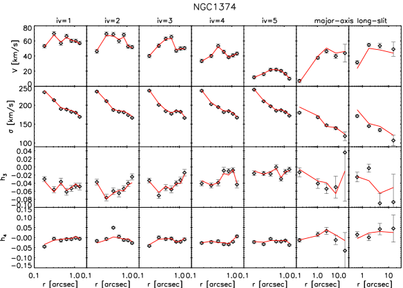
Figure 19: Kinematic data (black diamonds) and the best-fit model (red lines) for NGC 1374. The first to fifth columns are for SINFONI data with increasing angle from major towards minor axis (see Fig. 2). The 6th and the 7th columns show both sides of the slit data along the major axis.

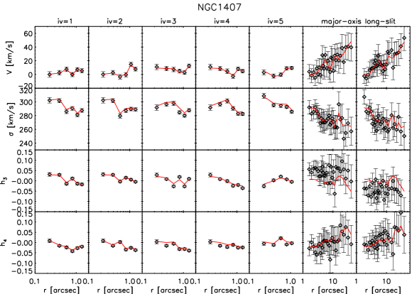
Figure 20: The same as Fig. 19 for NGC 1407. The 6th and the 7th columns display both sides of the major-axis slit data presented in Spolaor et al. (2008a).

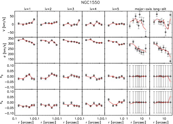
Figure 21: The same as Fig. 19 for NGC 1550. The 6th and the 7th columns display both sides of the major-axis slit data from Simien & Prugniel (2000).

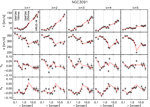
Figure 22: The same as Fig. 19 for NGC 3091. The dotted vertical lines mark the region covered by SINFONI 100 mas data (leftmost), SINFONI 250mas data (middle) and VIRUS-W data (rightmost).

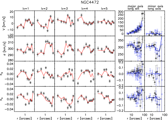
Figure 23: Kinematic data (diamonds) and the best-fit model (lines) for NGC 4472. The first to fifth columns display SINFONI data with increasing angle from major towards minor axis. The 6th column shows both sides of the major axis data from Bender, Saglia, & Gerhard (1994). The 7th column shows both sides of minor axis data from the same paper. The different colors represent data from different sides.

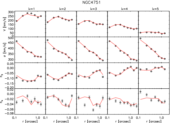
Figure 24: The same as Fig. 19 for NGC 4751. The complementary data are shown in the next figure.

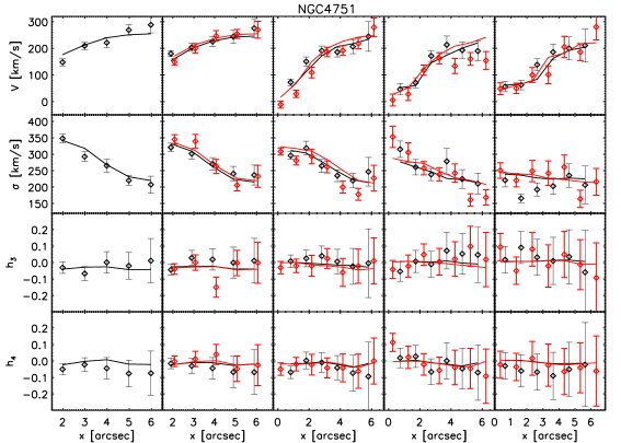
Figure 25: WiFeS kinematic data (diamonds) and the best-fit model (lines) for NGC 4751. Note that the Gauss-Hermite moments are not plotted as a function of radius but as a function of x-axis values (or projected radius onto the x-axis) of the datapoints. The leftmost to the rightmost columns show the pseudoslits in an ascending order of y-axis values. The black diamonds and lines correspond to the set of “pseudoslit” data having an angle of 5^∘ and the red color corresponds to the one with an angle of -5^∘ (see Section 3.2 and Fig. 7).

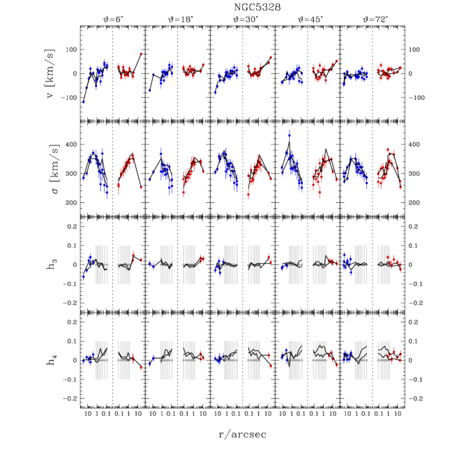
Figure 26: Kinematic data (circles) and the best-fit model (lines) for NGC 5328. The five columns represent the angular binning ($\vartheta$ is the angle between the bin and the major-axis). The VIRUS-W data points are included according to their bin centers. Over the SINFONI FoV we do not model the measured $h_{3}$ and $h_{4}$ but use $h_{3}=h_{4}=0$, $\Delta h_{3}=\Delta h_{4}=0.1$ (indicated in grey).

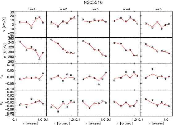
Figure 27: The same as Fig. 19 for NGC 5516. The complementary data are shown in the next figure.

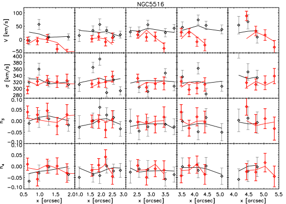
Figure 28: The same as Fig. 25 for NGC 5516. The black diamonds and lines correspond to the set of “pseudoslit” data having an angle of 108^∘ and the red color corresponds to the one with an angle of 72^∘ (see Section 3.2 and Fig. 9.)

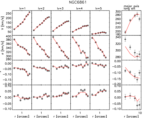
Figure 29: The same as Fig. 19 for NGC 6861. The 6th column shows the slit data along the major axis.

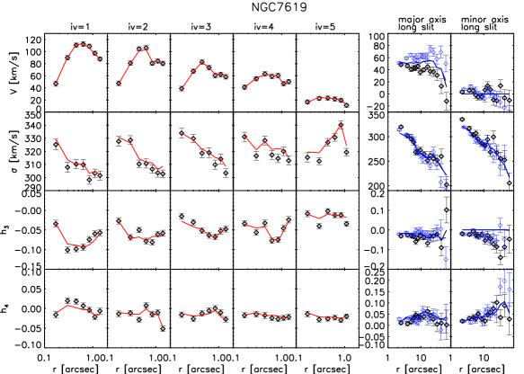
Figure 30: Kinematic data (diamonds) and the best-fit model (lines) for NGC 7619. The first to fifth columns display SINFONI data with increasing angle from major towards minor axis. The 6th column shows both sides of the major axis data from Pu, Saglia, Fabricius et al. (2010). The 7th column show both sides of minor axis data from the same paper. The different colors represent data from different sides.

References

- Abuter et al. (2006) Abuter, R., Schreiber, J., Eisenhauer, F., et al. 2006, New Astronomy Review, 50, 398
- Baes, Dejonghe & Buyle (2005) Baes, M., Dejonghe, H., & Buyle, P. 2005, A&A, 432, 411
- Beifiori et al. (2009) Beifiori, A., Sarzi, M., Corsini, E. M., et al. 2009, ApJ, 692, 856
- Bender (1990) Bender, R. 1990, A&A, 229, 441
- Bender & Moellenhoff (1987) Bender, R., & Moellenhoff, C. 1987, A&A, 177, 71
- Bender, Saglia, & Gerhard (1994) Bender, R., Saglia, R. P., & Gerhard, O. E. 1994, MNRAS, 269, 785
- Bernardi et al. (2006) Bernardi, M., et al. 2006, AJ, 131, 2018
- Binney & Tremaine (1987) Binney, J., & Tremaine, S. 1987, Galactic dynamics
- Blanton, Hogg, Bahcall et al. (2003) Blanton, M. R., Hogg, D. W., Bahcall, N. A., et al. 2003, ApJ, 592, 819
- Bonaccini et al. (2002) Bonaccini, D., Hackenberg, W. K., Cullum, M. J., et al. 2002, Proc. SPIE, 4494, 276
- Bonnet, Ströbele, Biancat-Marchet et al. (2003) Bonnet, H., Ströbele, S., Biancat-Marchet, F., et al. 2003, in SPIE Conf. Ser., Society of Photo-Optical Instrumentation Engineers (SPIE) Conference Series, vol. 4839, ed. P. L. Wizinowich & D. Bonaccini, 329–343
- Burstein et al. (1987) Burstein, D., et al. 1987, ApJSS, 64,601
- Caon, Capaccioli, & D’Onofrio (1994) Caon, N., Capaccioli, M., & D’Onofrio, M. 1994, A&AS, 106, 199
- Cappellari & Copin (2003) Cappellari, M., & Copin, Y. 2003, MNRAS, 342, 345
- Cappellari, McDermid, Alatalo et al. (2012) Cappellari, M., McDermid, R. M., Alatalo, K., et al. 2012, Nature, 484, 485
- Cappellari et al. (2006) Cappellari, M., et al. 2006, MNRAS, 366, 1126
- Conroy & van Dokkum (2012) Conroy, C., & van Dokkum, P. G. 2012, ApJ, 760, 71
- Cretton et al. (1999) Cretton, N., de Zeeuw, P. T., van der Marel, R. P., & Rix, H.-W. 1999, ApJS, 124, 383
- Davies (2007) Davies, R. I. 2007, MNRAS, 375, 1099
- Djorgovski (1985) Djorgovski, S. B. 1985, Surface photometry of early-type galaxies, Ph.D. thesis, California Univ., Berkeley.
- D’Onofrio, Zaggia, Longo et al. (1995) D’Onofrio, M., Zaggia, S. R., Longo, G., et al. 1995, A&A, 296, 319
- Dopita, Hart, McGregor et al. (2007) Dopita, M., Hart, J., McGregor, P., et al. 2007, Ap&SS, 310, 255
- Dopita, Rhee, Farage et al. (2010) Dopita, M., Rhee, J., Farage, C., et al. 2010, Ap&SS, 327, 245
- Eisenhauer et al. (2003) Eisenhauer, F., et al. 2003, The Messenger, 113, 17
- Emsellem, Cappellari, Krajnović et al. (2007) Emsellem, E., Cappellari, M., Krajnović, D., et al. 2007, MNRAS, 379, 401
- Emsellem, Cappellari, Krajnović et al. (2011) Emsellem, E., Cappellari, M., Krajnović, D., et al. 2011, MNRAS, 414, 888
- Fabricius, Grupp, Bender et al. (2012) Fabricius, M. H., Grupp, F., Bender, R., et al. 2012, in Society of Photo-Optical Instrumentation Engineers (SPIE) Conference Series, Society of Photo-Optical Instrumentation Engineers (SPIE) Conference Series, Proc. SPIE, 8446,
- Fabricius, Saglia, Fisher et al. (2012) Fabricius, M. H., Saglia, R. P., Fisher, D. B., et al. 2012, ApJ, 754, 67
- Ferrarese & Merritt (2000) Ferrarese, L., & Merritt, D. 2000, ApJ, 539, L9
- Gebhardt et al. (2011) Gebhardt, K., Adams, J., Richstone, D., et al. 2011, ApJ, 729, 119
- Gebhardt & Thomas (2009) Gebhardt, K., & Thomas, J. 2009, ApJ, 700, 1690
- Gebhardt et al. (2000a) Gebhardt, K., et al. 2000a, ApJ, 539, L13
- Gebhardt et al. (2000b) Gebhardt, K., et al. 2000b, AJ, 119, 1157
- Gebhardt et al. (2003) Gebhardt, K., et al. 2003, ApJ, 583, 92
- Gössl & Riffeser (2002) Gössl, C. A., & Riffeser, A. 2002, A&A, 381, 1095
- Grützbauch et al. (2005) Grützbauch, R., Annibali, F., Bressan, A., et al. 2005, MNRAS, 364, 146
- Gültekin, Richstone, Gebhardt et al. (2009) Gültekin, K., Richstone, D. O., Gebhardt, K., et al. 2009, ApJ, 695, 1577
- Gültekin et al. (2009) Gültekin, K., et al. 2009, ApJ, 698, 198
- Holtzman, Burrows, Casertano et al. (1995) Holtzman, J. A., Burrows, C. J., Casertano, S., et al. 1995, PASP, 107, 1065
- Hopkins, Hernquist, Cox et al. (2006) Hopkins, P. F., Hernquist, L., Cox, T. J., et al. 2006, ApJS, 163, 1
- Jardel et al. (2011) Jardel, J. R., Gebhardt, K., Shen, J., et al. 2011, ApJ, 739, 21
- Kelly (2007) Kelly, B. C. 2007, ApJ, 665, 1489
- Kelly & Merloni (2012) Kelly, B. C., & Merloni, A. 2012, Advances in Astronomy, 2012
- Kormendy, Fisher, Cornell et al. (2009) Kormendy, J., Fisher, D. B., Cornell, M. E., et al. 2009, ApJS, 182, 216
- Kormendy & Richstone (1995) Kormendy, J., & Richstone, D. 1995, ARAA, 33, 581
- Kormendy & Ho (2013) Kormendy, J., & Ho, L. C. 2013, ARAA, in press
- Krajnović, Bacon, Cappellari et al. (2008) Krajnović, D., Bacon, R., Cappellari, M., et al. 2008, MNRAS, 390, 93
- Krajnović et al. (2011) Krajnović, D., Emsellem, E., Cappellari, M., et al. 2011, MNRAS, 414, 2923
- Krist et al. (2011) Krist, J. E., Hook, R. N., & Stoehr, F. 2011, Proc. SPIE, 8127
- Lauer et al. (2007a) Lauer, T. R., et al. 2007a, ApJ, 662, 808
- Lauer, Tremaine, Richstone et al. (2007b) Lauer, T. R., Tremaine, S., Richstone, D., et al. 2007b, ApJ, 670, 249