Multi-pulse phase resetting curves

Abstract

In this paper, we introduce and systematically study, in terms of phase response curves (PRC), the effect of a dual pulse excitation on the dynamics of an autonomous oscillator. Specifically, we test the deviations from a linear summation of phase advances from two small perturbations. We derive analytically a correction term, which generally appears for oscillators whose intrinsic dimensionality is greater than one. We demonstrate this effect in case of the Stuart-Landau model, and also in various higher dimensional neuronal model. The non-linear correction is found to be proportional to the square of the perturbation. This deviation from the superposition principle needs to be taken into account in studies of networks of pulse-coupled oscillators. Further, this deviation could be used for verification of oscillator models via a dual pulse excitation.

I Introduction

The weakly connected oscillator theory is often used to show conditions under which the oscillators are synchronized Kuramoto (1984). In this theory, small perturbations do not influence the amplitude of the oscillator, however they have a significant effect on its phase. This allows one for a drastic reduction in the description of the oscillator: instead of operating with the original, possibly high- dimensional set of equations, only one phase variable is used for each oscillator. Using the phase description alone, it is possible to find the conditions when oscillators are synchronized, provided the phase reduction is accurate enough, what is the case if the coupling is weak. One of the assumptions used in this approach is the principle of superposition, which states that the effect of several small perturbations on the period of the oscillation could be considered independently, and then summed.

In this paper, we examined the phase dynamics beyond the superposition principle. More precisely, we consider the effect of two relatively small perturbations on the phase for various types of oscillators. Our main tool in the description of the phase dynamics is the Phase Response Curve (PRC, $\delta{\varphi}$) which is widely used in both theoretical and experimental studies, especially in the field of neuroscience Winfree (1980); Kuramoto (1984); Glass and Mackey (1988); Canavier (2006); Schultheiss et al. (2012). The PRC measures the shift of the phase of the oscillator due to an external pulse, in dependence on the phase at which the pulse is applied. Or, in terms of the oscillator period, the PRC measures the local change in the period of the oscillator due to a pulse perturbation at various time points within the period. The oscillation can either advance or delay based on the sign of the PRC. To determine the PRC, one often performs an experiment just according to the definition of the PRC; this can be accomplished for individual biological neurons Galán et al. (2005) and for complex oscillating systems like those responsible for circadian rhythms in the brain Khalsa et al. (2003); Hilaire et al. (2012), see Refs. Phoka et al. (2010); Ikeda et al. (1983); Abramovich-Sivan and Akselrod (1998) for other biophysical examples. Furthermore, the PRC concept can be applied not only to individual oscillators, but to collective modes as well Ko and Ermentrout (2009); Levnajić and Pikovsky (2010).

The shape of the PRC curve is shown to be critical for the synchronization properties of the oscillator networks Achuthan and Canavier (2009). However, in the synchronization problem, an oscillator is subject not just to one external pulse, but to a series of pulses from the external force or another oscillator (or several other oscillators if more then two oscillators are coupled). Thus, in order to apply the PRC concept in such a situation, one has to know how the oscillator responds to a series of pulses. If the superposition principle holds, then the sum of two small perturbations will independently influence the period of the oscillator according to the PRCs for single inputs, and thus can be linearly added to predict the overall phase shift. However, generally one expects deviation from this simple superposition if the perturbations are not small. In this paper we systematically consider the effect of two pulses on the oscillator’s phase, and characterize the deviations from the pure superposition as nonlinear effects. We illustrate these effects also for several realistic models of neuron dynamics.

II Phase dynamics and definition of multi-pulse PRC

II.1 Pure phase dynamics

We start with the simplest case where the oscillator is described just by one variable, the phase $\varphi$ (to be assumed $2\pi$-periodic) that grows uniformly in time

$$\dot{\varphi}=\omega$$ (1)

Suppose that the action of a forcing pulse with strength $\varepsilon$ is described by the standard PRC $\varepsilon S(\varphi,\varepsilon)$ (here dependence of $S$ on $\varepsilon$ accounts for nonlinear terms, so that $S(\varphi,0)$ is the linear PRC). Consider now the action of two pulses, at times $t_{0}$ and $t_{0}+\tau$, having strengths $\varepsilon_{0}$ and $\varepsilon_{1}$, respectively. Just after the first pulse

$$\varphi_{+}(t_{0})=\varphi(t_{0})+\varepsilon_{0}S(\varphi(t_{0}),\varepsilon_{0})\;.$$

Just prior to the second pulse the phase is

$$\varphi(t_{0}+\tau)=\varphi_{+}(t_{0})+\omega\tau=\varphi(t_{0})+\omega\tau+\varepsilon_{0}S(\varphi(t_{0}),\varepsilon_{0})\;,$$

and after the second pulse

$$\varphi_{+}(t_{0}+\tau)=\varphi(t_{0})+\omega\tau+\varepsilon_{0}S(\varphi(t_{0}),\varepsilon_{0})+\varepsilon_{1}S(\varphi(t_{0})+\omega\tau+\varepsilon_{0}S(\varphi(t_{0}),\varepsilon_{0}),\varepsilon_{1})\;.$$

Thus, the overall effect of two pulses

$$\Delta\varphi=\varepsilon_{0}S(\varphi(t_{0}),\varepsilon_{0})+\varepsilon_{1}S[\varphi(t_{0})+\omega\tau+\varepsilon_{0}S(\varphi(t_{0}),\varepsilon_{0}),\varepsilon_{1}]$$ (2)

can be simply calculated via the superposition of two single-pulse PRC functions $\varepsilon S(\varphi,\varepsilon)$. In the linear approximation, where $\varepsilon S(\varphi,\varepsilon)\approx\varepsilon S(\varphi,0)$ one obtains just the sum

$$\Delta\varphi\approx\varepsilon_{0}S(\varphi(t_{0}),0)+\varepsilon_{1}S(\varphi(t_{0})+\omega\tau,0)\;.$$

II.2 General consideration

Now we consider a general situation where periodic oscillations are described by a limit cycle $\mathbf{x}_{0}(t)$ in a generally $N$-dimensional phase space. The crucial notion simplifying the consideration, is that of isochrons Guckenheimer (1975), which are submanifolds of codimension one foliating the phase space and having the same phase as the corresponding points on the limit cycle. This allows one to represent the phase space as $(\mathbf{a},\varphi)$ where $\mathbf{a}$ is an $(N-1)$-dimensional “amplitude”, and the phase obeys the same equation (1). Without loss of generality, to simplify notations, we can assume that on the limit cycle the amplitude vanishes $\mathbf{a}=0$.

In terms of the phase and the amplitude, a pulse that kicks the system resets the state $(\mathbf{a},\varphi)$ as

$$\varphi \to\varphi+\varepsilon\Phi(\mathbf{a},\varphi,\varepsilon)\;,$$

$$\mathbf{a} \to\mathbf{a}+\varepsilon\mathbf{A}(\mathbf{a},\varphi,\varepsilon)\;,$$

where again $\Phi(\mathbf{a},\varphi,0)$ and $\mathbf{A}(\mathbf{a},\varphi,0)$ correspond to a linear approximation. The usual PRC is defined for the initial state on the limit cycle ($\mathbf{a}=0$), so $S(\varphi,\varepsilon)=\Phi(0,\varphi,\varepsilon)$. We now apply as above two pulses at times $t_{0}$ and $t_{0}+\tau$, assuming that the system is initially on the limit cycle. Then after the first pulse

$$\varphi_{+}(t_{0})=\varphi(t_{0})+\varepsilon_{0}S(\varphi(t_{0}),\varepsilon_{0}),\qquad\mathbf{a}_{+}(t_{0})=\varepsilon_{0}\mathbf{A}(0,\varphi(t_{0}),\varepsilon_{0})\;.$$

Just prior to the second pulse

$$\varphi(t_{0}+\tau) =\varphi_{+}(t_{0})+\omega\tau=\varphi(t_{0})+\omega\tau+\varepsilon_{0}S(\varphi(t_{0}),\varepsilon_{0}),$$

$$\mathbf{a}(t_{0}+\tau) =\mathcal{L}^{\tau}(t_{0})\mathbf{a}_{+}(t_{0})=\mathcal{L}^{\tau}(t_{0})\varepsilon_{0}\mathbf{A}(0,\varphi(t_{0}),\varepsilon_{0})\;,$$

where $\mathcal{L}^{\tau}$ is the operator describing the evolution of the amplitudes. After the second pulse the new phase is

$$\varphi_{+}(t_{0}+\tau)=\varphi(t_{0}+\tau)+\varepsilon_{1}\Phi(\mathbf{a}(t_{0}+\tau),\varphi(t_{0}+\tau),\varepsilon_{1})$$

and the overall phase shift due to two pulses (two-pulse PRC) is

$$\delta\varphi=\varepsilon_{0}S(\varphi(t_{0}),\varepsilon_{0})+\varepsilon_{1}\Phi(\mathbf{a}(t_{0}+\tau),\varphi(t_{0}+\tau),\varepsilon_{1})\;.$$ (3)

Comparing this with expression (2) we see that now the effect is not a superposition of two PRCs, but contains the amplitude-dependent phase reset function $\Phi$. The difference between expressions (2) and (3) gives the nontrivial effect of multiple pulses on the phase of the oscillator as the nonlinear correction term $\Delta$:

$$\Delta=\delta\varphi-\Delta\varphi=$$ (4)

$$=\varepsilon_{1}\Phi(\mathcal{L}^{\tau}(t_{0})\varepsilon_{0}\mathbf{A}(0,\varphi(t_{0}),\varepsilon_{0}),\varphi(t_{0})+\omega\tau+S(\varphi(t_{0}),\varepsilon_{0}),\varepsilon_{1})$$

$$-\varepsilon_{1}S(\varphi(t_{0})+\omega\tau+S(\varphi(t_{0}),\varepsilon_{0}),\varepsilon_{1})$$

$$=\varepsilon_{1}\Phi(\mathcal{L}^{\tau}(t_{0})\varepsilon_{0}\mathbf{A}(0,\varphi(t_{0}),\varepsilon_{0}),\varphi(t_{0})+\omega\tau+S(\varphi(t_{0}),\varepsilon_{0}),\varepsilon_{1})$$

$$-\Phi(0,\varphi(t_{0})+\omega\tau+S(\varphi(t_{0}),\varepsilon_{0}),\varepsilon_{1})\;.$$

From this expression one can see that the result essentially depends on the action of the amplitude evolution operator $\mathcal{L}^{\tau}$: if $\mathcal{L}^{\tau}(t_{0})\mathbf{A}\approx 0$, then the correction (4) vanishes. Thus, the nontrivial effect of the two-pulse excitation of an oscillator depends crucially on the relation between the time interval between the pulses $\tau$ and the relaxation time of the amplitude $t_{a}$ (characteristic time scale of the amplitude evolution operator $\mathcal{L}$), it is mostly pronounced if $\tau\lesssim t_{a}$. If the amplitude is multidimensional, $t_{a}$ is the time of most slow decay.

In the leading order in the powers of $\varepsilon_{0},\varepsilon_{1}$, we can represent the nonlinear correction as

$$\Delta\approx\varepsilon_{1}\varepsilon_{0}\mathcal{L}_{l}^{\tau}(t_{0})\mathbf{A}(0,\varphi(t_{0}),0)\frac{\partial}{\partial\mathbf{a}}\Phi(\mathbf{a},\varphi(t_{0})+\omega\tau+S(\varphi(t_{0}),0),0)|_{\mathbf{a}=0}\;,$$ (5)

where $\mathcal{L}_{l}$ is the linearized evolution operator for the amplitudes, which describes their relaxation to zero $\sim\exp[-t/t_{a}]$.

This can be generalized to $n$ pulses with amplitudes ($\varepsilon_{0},\ldots\varepsilon_{n-1},\varepsilon_{n}$) and different time shifts between them $(\tau_{0},\ldots,\tau_{n-1})$. Then the leading terms will be quadratic ones ($\sim\varepsilon_{0}\varepsilon_{1}\;,\varepsilon_{0}\varepsilon_{2}\;,\varepsilon_{1}\varepsilon_{2}\;,\ldots$), while also higher-order corrections (e.g. $\sim\varepsilon_{0}\varepsilon_{1}\varepsilon_{2}$) will appear. Mostly important will be nonlinear terms including neighboring pulses, because, as argued above, the effect decreases with the time interval between the pulses. Another straightforward generalization is the case where two pulses are different and are described by functions $\Phi_{0},\\ mathbf{A}_{0},\Phi_{1},\mathbf{A}_{1}$.

II.3 Example: a Stuart-Landau oscillator

The Stuart-Landau oscillator is a two-dimensional model described in polar coordinates as

$$\dot{R}=\mu R(1-R^{2})\;,\qquad\dot{\theta}=1+\alpha-\alpha R^{2}\;.$$

Here the frequency of the limit cycle, which is a circle with radius $R=1$, is normalized to one, parameter $\alpha$ describes nonisochronicity of oscillations, while $\mu$ is the relaxation rate of the amplitude. The phase $\varphi$ defined in the whole plane (except for the origin) is

$$\varphi=\theta-\frac{\alpha}{\mu}\ln R\;.$$

Evolution of the variables $R,\theta$ can be explicitly solved as

$$\begin{pmatrix}R(t)\\ \theta(t)\end{pmatrix}=U^{t-t_{0}}\begin{pmatrix}R(t_{0})\\ \theta(t_{0})\end{pmatrix}=\begin{pmatrix}[1+\frac{1-R(t_{0})^{2}}{R(t_{0})^{2}}e^{-2\mu(t-t_{0})}]^{-1/2}\\ \theta(t_{0})+t-t_{0}-\frac{\alpha}{2\mu}\ln(R(t_{0})^{2}+(1-R(t_{0})^{2})e^{-2\mu(t-t_{0})})\end{pmatrix}\;,$$

which defines the operator $\mathcal{L}$. We assume that the pulse is acting in direction $x$, i.e. at the pulse

$$R\cos\theta\to R\cos\theta+\epsilon,\qquad R\sin\theta\to R\sin\theta\;.$$

This fully describes the system, and one can find expressions for the PRCs $\Delta\varphi$ and $\delta\varphi$, see Appendix A. According to these formulas we calculated the nonlinear correction term $\Delta$ and plot it in Fig. 1. Here we take $\varepsilon_{0}=\varepsilon_{1}=0.1$ and present results for different $\mu$. As expected, the mostly pronounced effect is for small $\mu$.

For this equation it is possible to obtain the leading term in order $\sim\varepsilon_{0}\varepsilon_{1}$ in the expansion of the nonlinear correction term in the pulse strengths analytically (see Appendix A):

$$\Delta\approx\varepsilon_{0}\varepsilon_{1}(1+\frac{\alpha^{2}}{\mu^{2}})e^{-2\mu\tau}\cos\varphi_{0}\sin(\varphi_{0}+\tau)$$ (6)

This expression fits numerics very good for $\varepsilon\lesssim 0.01$.

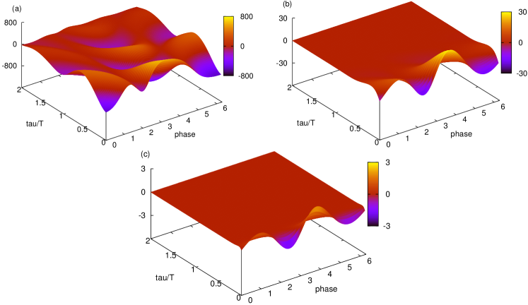
Figure 1: (color online) The normalized nonlinear effect of two-pulse action on the Stuart-Landau oscillator $\Delta\cdot\varepsilon^{-2}$ vs the phase $\varphi_{0}$ and the time shift between pulses $\tau$ (normalized by the cycle period), for $\varepsilon=0.1,\alpha=3$, and three different values of $\mu$ ($\mu=0.1$ in (a), $\mu=0.5$ in (b), and $\mu=2$ in (c)). For large $\mu$ the effect is pronounced for very small time intervals between two pulses only.

II.4 Example: a modified Stuart-Landau oscillator

Our second example is a modification of the Stuart-Landau oscillator proposed in Ermentrout et al. (2012):

$$\dot{R}=\mu R(1-R^{2})\;,\qquad\dot{\theta}=1-br\cos\theta+\alpha-\alpha R^{2}\;.$$ (7)

Here large values of parameter $b$ produce highly nonuniform growth of angle variable $\theta$, so that the relation between $\varphi$ and $\theta$ is strongly nonlinear. As a result, the isochrons crowd at the region around $\theta\approx 0$ where the evolution of $\theta$ is slow. Also the nonlinear correction term becomes very large at this region, as illustrated in Fig. 2

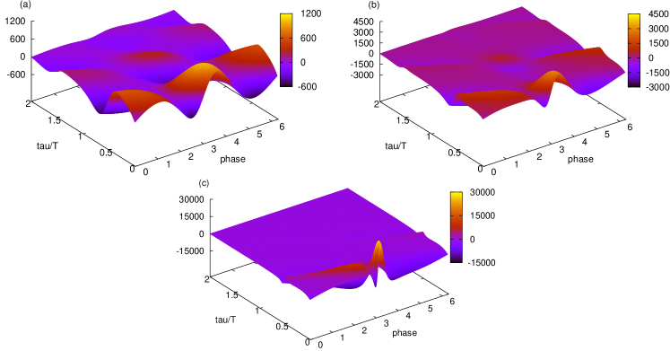
Figure 2: (color online) The same as fig. 1 but for the modified Stuart-Landau oscillator Eq. (7). Parameter values: (a) $\alpha=3,\mu=0.1,\varepsilon=0.01,b=0.3$; (b): $\alpha=3,\mu=0.1,\varepsilon=0.01,b=0.7$; (c): $\alpha=3,\mu=0.1,\varepsilon=0.001,b=0.95$.

III Neuron Models

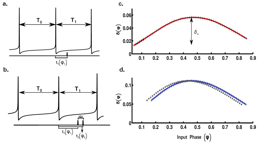
Figure 3: (color online) Figure illustrates how PRC is computed for a quadratic integrate fire neuron. a. Single pulse, b. Double pulse. $T_{0}$ is the original period when no input occurred, $T_{1}$ is the period when there was an input at time $t_{1}$ with input phase $\varphi_{1}=t_{1}/T_{0}$. c. PRC $\delta\varphi=(T_{0}-T_{1})/T_{0}$ for single input (black cross) along with its fit (solid red line ($\bar{\delta}_{1}(\varphi_{1})$)). d. PRC for 2 inputs with ISI=10ms. Gray points indicate the change in period against the first input; PRC with respect to the second input is plotted as black cross. The prediction from superposition principle is plotted as solid blue line ($\bar{\delta}_{1}(\varphi_{1})+\bar{\delta}_{1}(\varphi_{2})$).

The PRC is commonly used to describe neuron models. In this context, the PRC can characterize the properties of neurons, especially their synchronizability. In many systems a neuron receives inputs from many other neurons, therefore, it is critical to understand how multiple pulses affect the PRC response of neurons. Below we test four different neuron models for the dual pulse effect. Although generally the theory presented in section II.2 is applicable to spiking neurons as well, practically one does not follow the continuous phase of the oscillations, but focuses on the spiking events (these events are readily available in experiment, too). Therefore, for spiking neurons, the PRC and the non-linear correction term have to be measured in terms of the spike times as oppose to phase shifts at arbitrary points as done in previous section. It is convenient to normalize the correction term should by the peak to trough value of the PRC for single input as shown below. We first illustrate these definitions in Fig. 3, using the quadratic integrate-and-fire model Izhikevich (2007). (Note that traditionally in this context the phase $t/T_{0}$ and the PRC $\delta\varphi=(T_{1}-T_{0})/T_{0}$ are normalized by one and not by $2\pi$). This one- dimensional model corresponds to the pure phase dynamics as in section II.1, so it does not demonstrate nonlinear effects of deviations from the superposition.

In general, the models of neurons are classified based on their PRC curves as type I and II. The type I PRC, has only phase advance in response to perturbation, while type II PRC includes both phase delay and advance  Canavier (2006). We further considered both type I and II neuron models in this study. We tested Wang-Buzsáki model (type I, based on Wang and Buzsáki (1996)), the original Hodgkin-Huxley model (type II, based on Hodgkin and Huxley (1952)), and a modified Hodgkin-Huxley model (type I, based on Mainen and Sejnowski (1996)). The equations for all the models are given in the Appendix B. All of these models are three-dimensional which is required for any deviation from linear superposition.

To characterize the deviation from the superposition of two input pulses, we use the following quantity

$$\Delta_{p}=(\delta_{2}(\varphi_{2})-\bar{\delta}_{1}(\varphi_{1})-\bar{\delta}_{1}(\varphi_{2}))\frac{100}{\delta_{m}}$$ (8)

where, $\delta_{2}(\varphi_{2})$ is the measured PRC for the second pulse, $\bar{\delta}_{1}(\varphi_{1})$ and $\bar{\delta}_{1}(\varphi_{2})$ are the expected PRCs of single pulses, and $\delta_{m}$ is the amplitude of the single-pulse PRC (this normalization provides a better visualization of the deviation from the superposition of single-pulse PRCs). We present the results for the three neuron models in Figs. 4-6, where the main dependence of of $\Delta_{p}$ on the first input phase and on the interspike interval (ISI) between two applied pulses $\tau$ is depicted in panel c by a color coding.

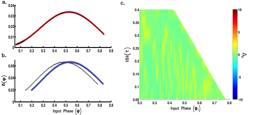
Figure 4: (color online) Wang-Buzsáki Model. a. PRC for single input along with its fit (solid red line) ($\delta(\varphi)=(T_{0}-T_{1})/T_{0}$). b. PRC for 2 inputs with ISI=10ms. Gray points indicate the PRC with respect to the first input and PRC with respect to second input is plotted as black cross. The prediction from superposition principle is plotted as solid blue line. c. The deviation from linear superposition ($\Delta_{p}$) for different ISIs.

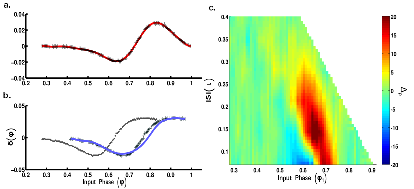
Figure 5: (color online) Original Hodgkin-Huxley Model. Legend same as Fig 4

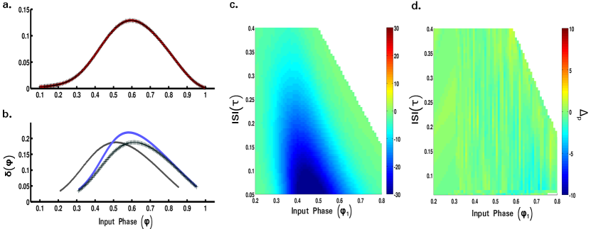
Figure 6: (color online) Modified Hodgkin-Huxley Model. a.-c.Legend same as Fig 4 d. Error for modified Hodgin-Huxley model with slower evolution, $\rho$= 0.5 (see Appendix B for definition of $\rho$)

We observed that some neuron models show pronounced nonlinear effects, as the two-pulse response deviates from the expected PRC based on superposition principle, while for other models the linear superposition was able to predict the PRC for two-pulses accurately. The Wang-Buzsáki model (4) appears to be of the latter type, while both the original Hodgkin-Huxley system (5) and its modified version (6) show nonlinear effects in two-pulse PRC. The Wang-Buzsáki and modified Hodgkin-Huxley model had type I PRC, the original Hodgkin-Huxley model had type II PRC, suggesting that there is no relationship between the type of PRC and the origin of this deviation. Further, the bifurcation type for spiking from the resting state also did not determine the existence of error, since the Wang-Buzsáki model and the modified Hodgkin-Huxley model possess a saddle-node bifurcation, while the original Hodgkin-Huxley model demonstrates an Andronov-Hopf bifurcation.

There were two main findings from the analytical results of section II that can be tested with the neuronal models presented in this section. The first result was that the non-linear correction term was proportional to the square of the perturbation 6. We tested this in the modified Hodgkin-Huxley model and observed similar qualitative results (Fig. 7). Second, the decay time constant of the amplitude term in the oscillator due to perturbation was inversely proportional to the non-linear correction term (4). Thus, a slower dynamics of the neuron will lead to lower error. The modified neuron model also showed reduced error when the dynamics was slowed (Fig 6). Thus, the main features of general limit cycle oscillators, and in particular of Stuart-Landau oscillator, could be qualitatively extended to some of the neuron models.

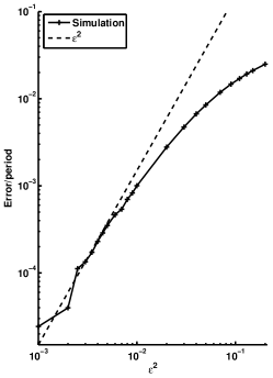
Figure 7: Relationship between $\epsilon^{2}$ and $\Delta$ / period. The division by period was used to compare with the Landau-Stewart oscillator simulations and does not change the relationship between $\epsilon^{2}$ and $\Delta$, since period was same for all $\epsilon^{2}$ .

IV Conclusion

In this paper we have developed a theory of a response of an autonomous oscillator to two-pulse perturbation. We found that the action of two pulses generally deviates from the superposition of two one-pulse responses, and this nonlinear effect, which is proportional to the product of the perturbations’ amplitudes, significantly depends on the relation of the interval between the pulses and the relaxation time of the oscillator. For fast relaxation and large time interval between the pulses, the nonlinear effect vanishes. We have demonstrated this property for several models: the standard Stuart-Landau oscillator, the modified version for this oscillator with a highly non-uniform motion over the cycle, and for three neuron models, including the classical Hodgkin-Huxley system.

We stress here that in our study, the term “nonlinearity” of the PRC has been used in two contexts. For a one-pulse PRC, nonlinearity means, that the phase response cannot be represented as an amplitude of the pulse multiplied by a function of the phase; in particular, the form of the curve may depend on the pulse amplitude. For two pulses, we use term “nonlinearity” to describe a deviation from the superposition principle, this effect in the leading order is proportional to the product of the pulses’ amplitudes. We have shown that the nonlinearity of the single-pulse PRC does not necessarily lead to the the nonlinearity for a two-pulse excitation: the purely phase model of section II.1 is a good illustration of this. Both nonlinear effects may distort a simple picture of the neuron’s dynamics under external forcing. In particular, in Izhikevich (2007) it was suggested that relatively weak noisy current to neuron can be applied to obtain the PRC, by solving the equation that relates the infinitesimal (linear) PRC to the external voltage through optimization methods. However, this method does not account for the non-linear correction which we showed in this study. In some neurons, we showed that the non-linear effect could have significant effect on the multi-pulse PRC compared to the single pulse PRC, and thus the continuous perturbation method may produce erroneous results. Thus, further studies are required to validate the method proposed in Izhikevich (2007).

We see two main application fields of our approach. First, it can be used for a diagnostics of oscillators. While the usual PRC allows to characterize sensitivity of the phase to an external action, the nonlinear terms in the two-pulse response allow to characterize relaxation processes. In particular, one-pulse PRCs of the Wang-Buzsáki model and of the modified Hodgkin-Huxley model are very similar (cf. Figs. 4a and 6a), but their two-pulse PRCs are completely different; this may be useful for designing models to fit experimental data. Two-pulse PRC can be estimated from experimental data and this information can be used to design optimally a model that provides a best description of the data. The second field of application is in the incorporating these effects in the synchronization theory of pulse coupled oscillators. Indeed, in a network an oscillator usually experiences inputs from many other units, and in the absence of synchrony the time intervals between the incoming pulses can be rather small. In this case the nonlinear "interference" of the actions is mostly pronounced, and may contribute significantly to the synchronization properties.

Appendix A PRC for Stuart-Landau oscillator

We briefly outline the majors steps in obtaining the approximate non-linear correction term for Stuart-Landau oscillator using an expansion in $\varepsilon$. Several intermediate steps are not shown to make presentation brief. Section II.3 provides the phase equation and the evolution operator for Stuart-Landau oscillator.

At $t=0$, let $R=1$, $\theta=\theta_{0}$. After $\varepsilon_{0}$ pulse at $t=0$, $\tilde{R}=\sqrt{(\cos\theta_{0}+\epsilon_{0})^{2}+\sin^{2}\theta_{0})}$, $\tilde{\theta}_{0}=\arctan(\sin\theta_{0}/(\cos\theta_{0}+\epsilon_{0}))$, which upon expansion gives, $\tilde{R}=1+\epsilon_{0}\cos\theta_{0}+\epsilon_{0}^{2}(\frac{\sin^{2}\theta_{0}}{2})+O(\varepsilon^{3})$ and $\tilde{\theta}_{0}=\theta_{0}-\epsilon_{0}\sin\theta_{0}+\epsilon_{0}^{2}\sin\theta_{0}\cos\theta_{0}+O(\varepsilon^{3})$. From here we ignore all, $O(\varepsilon^{3})$, cubic and higher order terms.

The phase shift due to $\varepsilon_{0}$ pulse is,

$$\Delta\varphi_{0}=\tilde{\theta}_{0}-\theta_{0}-\frac{\alpha}{\mu}\ln\tilde{R}=\arctan(\sin\theta_{0}/(\cos\theta_{0}+\epsilon_{0}))-\theta_{0}-\frac{\alpha}{\mu}\ln\sqrt{(\cos\theta_{0}+\epsilon_{0})^{2}+\sin^{2}\theta_{0})}$$

$$\Delta\varphi_{0}=\arctan\frac{-\epsilon_{0}\sin\theta_{0}}{1+\epsilon_{0}\cos\theta_{0}}-\frac{\alpha}{\mu}\ln\sqrt{(\cos\theta_{0}+\epsilon_{0})^{2}+\sin^{2}\theta_{0})}$$

$$\approx-\epsilon_{0}(\sin\theta_{0}+\frac{\alpha}{\mu}\cos\theta_{0})+\frac{1}{2}\epsilon_{0}^{2}(\sin 2\theta_{0}+\frac{\alpha}{\mu}\cos 2\theta_{0})$$

At time $\tau$

$$\begin{pmatrix}R(\tau)\\ \theta(\tau)\end{pmatrix}=U^{\tau}\begin{pmatrix}\tilde{R}\\ \tilde{\theta}_{0}\end{pmatrix}$$

$$\theta(\tau) =\tilde{\theta}_{0}+\tau-\frac{\alpha}{2\mu}\ln\left(\tilde{R}^{2}+(1-\tilde{R}^{2})\exp(-2\mu\tau)\right)$$

$$\approx\tau+\theta_{0}-\epsilon_{0}\sin\theta_{0}+\epsilon_{0}^{2}\sin\theta_{0}\cos\theta_{0}-\frac{\alpha}{2\mu}\ln\left((1+2\epsilon_{0}\cos\theta_{0}+\epsilon_{0}^{2})+(-2\epsilon_{0}\cos\theta_{0}-\epsilon_{0}^{2})e^{-2\mu\tau}\right)$$

$$\approx\tau+\theta_{0}-\epsilon_{0}[\sin\theta_{0}+\frac{\alpha}{\mu}\cos(1-e^{-2\mu\tau})]+\epsilon_{0}^{2}[\sin\theta_{0}\cos\theta_{0}-\frac{\alpha}{2\mu}(1-e^{-2\mu\tau}-2\cos^{2}\theta_{0}(1-e^{-2\mu\tau})^{2})]$$

$$\equiv\tau+\theta_{0}-\epsilon_{0}E+\epsilon_{0}^{2}F$$

$$R(\tau) =\big{[}\frac{\tilde{R}^{2}}{\tilde{R}^{2}+(1-\tilde{R}^{2})e^{-2\mu\tau}}\big{]}^{1/2}\approx\big{[}\frac{1+2\epsilon_{0}\cos\theta_{0}+\epsilon_{0}^{2}}{1+2\epsilon_{0}\cos\theta_{0}+\epsilon_{0}^{2}+(-2\epsilon_{0}\cos\theta_{0}-\epsilon_{0}^{2})e^{-2\mu\tau}}\big{]}^{1/2}$$

$$R(\tau)^{2} \approx\frac{1+2\epsilon_{0}\cos\theta_{0}+\epsilon_{0}^{2}}{1+2\epsilon_{0}\cos\theta_{0}(1-e^{-2\mu\tau})+\epsilon_{0}^{2}(1-e^{-2\mu\tau})}$$

$$\approx 1+2\epsilon_{0}\cos\theta_{0}e^{-2\mu\tau}-4\epsilon_{0}^{2}\cos^{2}\theta_{0}(1-e^{-2\mu\tau})+\epsilon_{0}^{2}e^{-2\mu\tau}+4\epsilon_{0}^{2}\cos^{2}\theta_{0}(1-e^{-2\mu\tau})^{2}$$

$$\approx 1+2\epsilon_{0}\cos\theta_{0}e^{-2\mu\tau}+\epsilon_{0}^{2}[-4\cos^{2}\theta_{0}(1-e^{-2\mu\tau})e^{-2\mu\tau}+e^{-2\mu\tau}]$$

$$\equiv 1+\epsilon_{0}C+\epsilon_{0}^{2}D$$

After the second pulse ($\varepsilon_{1}$) at time $\tau$, $\hat{R}(\tau)=\sqrt{(R(\tau)\cos\theta(\tau)+\epsilon_{1})^{2}+(R(\tau)\sin\theta(\tau))^{2}}$ and $\hat{\theta}(\tau)=\arctan(R(\tau)\sin\theta(\tau)/(R(\tau)\cos\theta(\tau)+\epsilon_{1}))$. So the final phase shift is, $\Delta\varphi_{0,1}=\hat{\theta}(\tau)-\theta_{0}-\tau-\frac{\alpha}{2\mu}\ln\hat{R}^{2}(\tau)$, which needs to be compared to prediction from linear superposition which is given as $\Delta\varphi_{0}+\Delta\varphi_{1}$. We first expand $\cos\theta(\tau)$, $\hat{R}(\tau)$, $\hat{\theta}(\tau)$, since it is used in the comparison as,

$$\cos\theta(\tau) =\cos(\tau+\theta_{0}-\epsilon_{0}E+\epsilon_{0}^{2}F)$$

$$\approx\cos(\tau+\theta_{0})-\epsilon_{0}E\sin(\tau+\theta_{0})+\epsilon_{0}^{2}(-\frac{1}{2}E^{2}\cos(\tau+\theta_{0})-F\sin(\tau+\theta_{0}))$$

$$\hat{R}^{2}(\tau) =R^{2}(\tau)+2R(\tau)\epsilon_{1}\cos\theta(\tau)+\epsilon_{1}^{2}$$

$$\approx 1+\varepsilon_{0}C+\varepsilon_{0}^{2}D+2\varepsilon_{1}(1+\frac{1}{2}\varepsilon_{0}C)(\cos(\theta_{0}+\tau)+\varepsilon_{0}E\sin(\tau+\theta_{0}))+\epsilon_{1}^{2}$$

$$\hat{\theta}(\tau) =\arctan(R(\tau)\sin\theta(\tau)/(R(\tau)\cos\theta(\tau)+\varepsilon_{1}))$$

$$\approx\theta(\tau)-\frac{\varepsilon_{1}}{R(\tau)}\sin\theta(\tau)+\frac{\varepsilon^{2}}{R^{2}(\tau)}\sin\theta(\tau)\cos\theta(\tau)$$

$$\approx\tau+\theta_{0}+\epsilon_{0}E-\varepsilon_{1}\sin(\tau+\theta_{0})+\epsilon_{0}^{2}F+$$

$$\varepsilon_{0}\varepsilon_{1}[-\cos(\theta_{0}+\tau)E+\frac{1}{2}\sin(\theta_{0}+\tau)C]+\varepsilon_{1}^{2}\sin(\theta_{0}+\tau)\cos(\theta_{0}+\tau)$$

$$\Delta\varphi_{0}+\Delta\varphi_{1} =\Delta\varphi_{0}+\arctan\left(\frac{\sin(\theta_{0}+\Delta\varphi_{0}+\tau)}{(\cos(\theta_{0}+\Delta\varphi_{0}+\tau)+\epsilon_{1})}\right)-(\theta_{0}+\Delta\varphi_{0}+\tau)$$

$$-\frac{\alpha}{2\mu}\ln(\cos(\theta_{0}+\Delta\varphi_{0}+\tau)+\epsilon_{1})^{2}+\sin^{2}(\theta_{0}+\Delta\varphi_{0}+\tau)$$

$$\approx\Delta\varphi_{0}+\arctan\frac{-\epsilon_{1}\sin(\theta_{0}+\Delta\varphi_{0}+\tau)}{1+\epsilon_{1}\cos(\theta_{0}+\Delta\varphi_{0}+\tau)}-\frac{\alpha}{\mu}\ln(1+2\varepsilon_{1}\cos(\theta_{0}+\Delta\varphi_{0}+\tau)+\varepsilon_{1}^{2})$$

$$\approx-\epsilon_{0}(\sin\theta_{0}+\frac{\alpha}{\mu}\cos\theta_{0})+\frac{1}{2}\epsilon_{0}^{2}(\sin 2\theta_{0}+\frac{\alpha}{\mu}\cos 2\theta_{0})$$

$$+\varepsilon_{1}[\sin(\theta_{0}+\Delta\varphi_{0}+\tau)+\frac{\alpha}{\mu}\cos(\theta_{0}+\Delta\varphi_{0}+\tau)]$$

$$+\frac{1}{2}\varepsilon_{1}^{2}[\sin 2(\theta_{0}+\Delta\varphi_{0}+\tau)+\frac{\alpha}{\mu}\cos 2(\theta_{0}+\Delta\varphi_{0}+\tau)]$$

$$\Delta\varphi_{0,1} =\hat{\theta}(\tau)-\theta_{0}-\tau-\frac{\alpha}{2\mu}\ln\hat{R}^{2}(\tau)$$

$$=\epsilon_{0}E-\varepsilon_{1}\sin(\tau+\theta_{0})+\epsilon_{0}^{2}F+\varepsilon_{0}\varepsilon_{1}[-\cos(\theta_{0}+\tau)E+\frac{1}{2}\sin(\theta_{0}+\tau)C]$$

$$+\varepsilon_{1}^{2}\sin(\theta_{0}+\tau)\cos(\theta_{0}+\tau)$$

$$-\frac{\alpha}{2\mu}\ln[1+\varepsilon_{0}C+\varepsilon_{0}^{2}D+2\varepsilon_{1}(1+\frac{1}{2}\varepsilon_{0}C)(\cos(\theta_{0}+\tau)+\varepsilon_{0}E\sin(\tau+\theta_{0}))+\epsilon_{1}^{2}]$$

Finally, the difference between the prediction from superposition and actual phase reset (after substitutions) is given as,

$$\Delta\varphi_{0,1}-(\Delta\varphi_{0}+\Delta\varphi_{1})=$$

$$\epsilon_{0}[\sin\theta_{0}+\frac{\alpha}{\mu}\cos(1-e^{-2\mu\tau})]-\varepsilon_{1}\sin(\tau+\theta_{0})+\epsilon_{0}^{2}[\sin\theta_{0}\cos\theta_{0}-\frac{\alpha}{2\mu}(1-e^{-2\mu\tau}-2\cos^{2}\theta_{0}(1-e^{-2\mu\tau})^{2})]$$

$$+\varepsilon_{0}\varepsilon_{1}\big{[}-\cos(\theta_{0}+\tau)[\sin\theta_{0}+\frac{\alpha}{\mu}\cos(1-e^{-2\mu\tau})]+\frac{1}{2}\sin(\theta_{0}+\tau)2\cos\theta_{0}e^{-2\mu\tau}\big{]}+\varepsilon_{1}^{2}\sin(\theta_{0}+\tau)\cos(\theta_{0}+\tau)$$

$$-\frac{\alpha}{2\mu}\ln\Big{[}1+\varepsilon_{0}2\cos\theta_{0}e^{-2\mu\tau}+\varepsilon_{0}^{2}[-4\cos^{2}\theta_{0}(1-e^{-2\mu\tau})e^{-2\mu\tau}+e^{-2\mu\tau}]$$

$$\qquad\qquad+2\varepsilon_{1}(1+\frac{1}{2}\varepsilon_{0}2\cos\theta_{0}e^{-2\mu\tau})(\cos(\theta_{0}+\tau)+\varepsilon_{0}[\sin\theta_{0}+\frac{\alpha}{\mu}\cos(1-e^{-2\mu\tau})]\sin(\tau+\theta_{0}))+\epsilon_{1}^{2}\Big{]}$$

$$-\Big{[}-\epsilon_{0}(\sin\theta_{0}+\frac{\alpha}{\mu}\cos\theta_{0})+\frac{1}{2}\epsilon_{0}^{2}(\sin 2\theta_{0}+\frac{\alpha}{\mu}\cos 2\theta_{0})+\varepsilon_{1}[\sin(\theta_{0}+\Delta\varphi_{0}+\tau)$$

$$+\frac{\alpha}{\mu}\cos(\theta_{0}+\Delta\varphi_{0}+\tau)]+\frac{1}{2}\varepsilon_{1}^{2}[\sin 2(\theta_{0}+\Delta\varphi_{0}+\tau)+\frac{\alpha}{\mu}\cos 2(\theta_{0}+\Delta\varphi_{0}+\tau)]\Big{]}$$

which upon several steps of algebraic reductions and ignoring cubic or higher $\varepsilon$ terms gives,

$$\Delta\varphi_{0,1}-(\Delta\varphi_{0}+\Delta\varphi_{1})\approx\varepsilon_{0}\varepsilon_{1}(1+\frac{\alpha^{2}}{\mu^{2}})e^{-2\mu\tau}\cos\varphi_{0}\sin(\varphi_{0}+\tau)$$

Appendix B Neuron models

In these models $I_{stim}$ is the external input.

Wang-Buzáki Model Wang and Buzsáki (1996):

$$\dot{v} =-0.1(v+65)-9n^{4}(v+90)-35m_{\infty}^{3}h(v-55)-I_{Stim}$$ (9)

$$\dot{h} =(h_{\infty}-h)/h_{\tau}\qquad\dot{n}=(n_{\infty}-n)/n_{\tau}\qquad m_{\infty}=\alpha_{m}/(\alpha_{m}+\beta_{m})$$

$$\alpha_{m} =-(v+35)/(10(e^{-(v+35)/10}-1)),\qquad\beta_{m}=4e^{-(v+60)/18}$$

$$h_{\infty} =\alpha_{h}/(\alpha_{h}+\beta_{h}),\qquad h_{\tau}=1/(5(\alpha_{h}+\beta_{h}))\qquad\alpha_{h}=.07e^{-(v+58)/20},\qquad\beta_{h}=1/(e^{-(v+28)/10}+1)$$

$$n_{\infty} =\alpha_{n}/(\alpha_{n}+\beta_{n}),\qquad n_{\tau}=1/(5(\alpha_{n}+\beta_{n}))$$

$$\alpha_{n} =-.01(v+34)/(e^{-(v+34)/10}-1)\quad\beta_{n}=.125e^{-(v+44)/80}$$

Hodgkin-Huxley Model Hodgkin and Huxley (1952):

$$\dot{v} =-0.5(v+65)-36n^{4}(v+77)-120m_{\infty}^{3}h(v-50)-I_{Stim}$$ (10)

$$\dot{h} =(h_{\infty}-h)/h_{\tau}\qquad\dot{n}=(n_{\infty}-n)/n_{\tau}\qquad m_{\infty}=\alpha_{m}/(\alpha_{m}+\beta_{m})$$

$$\alpha_{m} =-0.1(v+40)/(e^{-(v+40)/10}-1)\qquad\beta_{m}=4e^{-(v+65)/18}$$

$$h_{\infty} =\alpha_{h}/(\alpha_{h}+\beta_{h})\qquad h_{\tau}=1/(\alpha_{h}+\beta_{h})\qquad\alpha_{h}=.07e^{-(v+65)/20}\qquad\beta_{h}=1/(e^{-(v+35)/10}+1)$$

$$n_{\infty} =\alpha_{n}/(\alpha_{n}+\beta_{h})\qquad n_{\tau}=1/(\alpha_{n}+\beta_{n})$$

$$\alpha_{n} =-.01(v+55)/(e^{-(v+55)/10}-1)\qquad\beta_{n}=.125e^{-(v+65)/80}$$

Modified Hodgkin-Huxley Model Mainen and Sejnowski (1996):

$$\dot{v} =(-0.0317(v+77.8)-30.032m_{\infty}^{3}h(v-49.8)-5.315n(v+100.4)-I_{Stim})/0.75$$ (11)

$$\dot{h} =-\rho(h-h_{\infty})/h_{\tau}\qquad\dot{n}=-\delta(n-n_{\infty})/n_{\tau}\qquad m_{\infty}=\alpha_{m}/(\alpha_{m}+\beta_{m})$$

$$\alpha_{m} =0.182(v+25)/(1-e^{-(v+25)/9})\qquad\beta_{m}=0.124(-v-25)/(1-e^{-(-v-25)/9})$$

$$h_{\infty} =\alpha_{h}/(\alpha_{h}+\beta_{h})\qquad h_{\tau}=1/(2.953(\alpha_{h}+\beta_{h}))$$

$$h_{\infty} =1/(1+e^{(v+55)/6.2})$$

$$\alpha_{h} =0.024(v+40)/(1-e^{-(v+40)/5});\beta_{h}=0.0091(-v-65))/(1-e^{-(-v-65)/5})$$

$$n_{\infty} =\alpha_{n}/(\alpha_{n}+\beta_{n})\qquad n_{\tau}=1/(2.953(\alpha_{n}+\beta_{n}))$$

$$\alpha_{n} =0.02*(v-25)/(1-e^{-(v-25)/9})\qquad\beta_{n}=-0.002*(v-25)/(1-e^{(v-25)/9})$$

where, $\rho$ is the factor which was reduced to 0.5 in Fig 6.