Exact Axisymmetric Solutions of the Maxwell Equations
in a Nonlinear Nondispersive Medium

Abstract

The features of propagation of intense waves are of great interest for theory and experiment in electrodynamics and acoustics. The behavior of nonlinear waves in a bounded volume is of especial importance and, at the same time, is an extremely complicated problem. It seems almost impossible to find a rigorous solution to such a problem even for any model of nonlinearity. We obtain the first exact solution of this type. We present a new method for deriving exact solutions of the Maxwell equations in a nonlinear medium without dispersion and give examples of the obtained solutions that describe propagation of cylindrical electromagnetic waves in a nonlinear nondispersive medium and free electromagnetic oscillations in a cylindrical cavity resonator filled with such a medium.

Wave propagation in nonlinear media is a fundamental and wide-ranging problem in physics Whitham (1974); Ablowitz and Segur (1981). The possible self-steepening and formation of shock discontinuities in large-amplitude pressure waves is well known in fluid mechanics, being a typical nonlinear phenomenon. A similar phenomenon (formation of surfaces of discontinuity for the electric and magnetic fields) can also be observed during propagation of intense electromagnetic waves in certain media, and there is an elegant physical analogy between the fluid mechanics and electrodynamics in this case. The discovery of materials with well-pronounced nonlinearity of electromagnetic properties (for example, ferrites and ferroelectrics) has attracted considerable attention to essentially nonlinear electromagnetic phenomena, and some important advances have been made Gaponov and Freidman (1959); Rosen (1965). Further theoretical progress, however, has met serious difficulties because such phenomena cannot be described satisfactorily by perturbation theory, and rigorous solutions of field equations are required in order to get theoretical predictions. In view of the above, finding new, physically important exact solutions of nonlinear partial differential equations (PDEs) that describe the behavior of waves in nonlinear media is very topical Polyanin and Zaitsev (2002); Fokas (2006). In most papers on the subject, plane nonlinear waves are considered. At the same time, features of propagation of nonlinear cylindrical and spherical waves, as well as the properties of the related nonlinear PDEs in the corresponding curvilinear coordinates, remain poorly studied.

In what follows, we present a new method for constructing exact axisymmetric solutions of the Maxwell equations in a nonlinear nondispersive medium. It is assumed that the medium considered lacks a center of inversion and the dependence of the electric displacement on the electric field can be approximated by an exponential function.

Consider electromagnetic fields in a loss-free nonmagnetic medium. With a view to analyzing uniaxial crystals, we assume that the medium possesses an axis of symmetry, hereafter taken as the $z$ axis of a cylindrical coordinate system ($r$, $\phi$, $z$). If the fields are independent of $\phi$ and $z$, the Maxwell equations admit solutions in which only the $E_{z}$ and $H_{\phi}$ components are nonzero ($E$ waves with respect to the symmetry axis). Restricting ourselves to consideration only of such solutions, we will also neglect dispersion effects and suppose that the relation of the displacement $D_{z}$ to the electric field $E_{z}$ is local in space and time. Denoting $E_{z}(r,t)$, $D_{z}(r,t)$, and $H_{\phi}(r,t)$ as $E$, $D$, and $H$, respectively, we can write equations for these functions in the form

$$\partial_{r}H+r^{-1}H=\varepsilon(E)\,\partial_{t}E,\quad\partial_{r}E=\mu_{0}\,\partial_{t}H,$$ (1)

where $\varepsilon(E)=dD/dE$. System (1) can be reduced to the nonlinear wave equation

$$\partial^{2}_{r}E+r^{-1}\partial_{r}E=\mu_{0}\,\partial_{t}(\varepsilon(E)\,\partial_{t}E).$$ (2)

It will be shown below that system (1) and Eq. (2) are integrated exactly if the function $\varepsilon(E)$ is chosen in the form

$$\varepsilon(E)=\epsilon_{0}\varepsilon_{1}\exp(\alpha E),$$ (3)

where $\varepsilon_{1}$ and $\alpha$ are certain constants. The longitudinal component of the electric displacement can be represented as $D=D_{0}+\alpha^{-1}\epsilon_{0}\varepsilon_{1}\left[\exp(\alpha E)-1\right]=D_{0}+\epsilon_{0}\varepsilon_{1}(E+\alpha E^{2}/2+\ldots)$, where $D_{0}=D(E=0)={\rm const}$. It is clear that function (3), as any theoretical model of nonlinearity, cannot be used in the entire range $0<|E|<\infty$. However, for moderately small electric fields observed in actual experiments ($|\alpha E|\ll 1$), the chosen dependence $D(E)$ correctly describes dielectric properties of certain media with accuracy up to terms of order $E^{2}$ inclusively. Since even powers of $E$ are present in the series expansion of $D$, the medium for which the dependence $\varepsilon(E)$ is approximated by function (3) does not possess a center of inversion Franken and Ward (1963). This is inherent in, e.g., uniaxial pyroelectric and ferroelectric crystals, provided that the $z$ axis is aligned with the crystallographic symmetry axis. The case where $D_{0}\neq 0$ corresponds to the presence of spontaneous polarization. The value of $\alpha$ can be obtained, for example, in experiments on microwave frequency doubling in ferroelectric crystals Ivanov (1980); Belokopytov (1995). Along with the medium properties, another factor leading to lack of a center of inversion can be the presence of a strong external electric field Franken and Ward (1963). For example, let an isotropic medium in which $D=\epsilon_{0}\varepsilon_{1}E_{z}+\chi^{(3)}E^{3}_{z}$, where $\chi^{(3)}={\rm const}$ Rosen (1965), be placed in a uniform static electric field ${\bf E}=E_{0}{\hat{\bf z}}_{0}$. Representing the total field as $E_{z}=E_{0}+E$, we obtain the term proportional to $E^{2}$ in the expansion of $D$. Thus, with appropriately chosen constants $D_{0}$, $\varepsilon_{1}$, and $\alpha$, formula (3) correctly describes dielectric properties of media lacking a center of inversion in the case of weak nonlinearity where we can restrict ourselves to the quadratic (in $E$) correction term to the linear dependence of $D$ on $E$.

Note that the forthcoming results can also be related to magnetic media lacking a center of inversion, such as ferromagnetic crystals. To this end, one should consider $H$ waves, for which $H_{z}\neq 0$ and $E_{\phi}\neq 0$, and put $dB_{z}/dH_{z}=\mu_{0}\mu_{1}\exp(\nu H_{z})$.

Let us use the following ansatz in system (1):

$$E=\alpha^{-1}(u-2\xi),\quad H=\varepsilon^{1/2}_{1}(Z_{0}\alpha)^{-1}\,e^{-\xi}(v-2\eta),$$ (4)

where $\xi={\rm ln}(r/r_{0})$, $\eta=t(\epsilon_{0}\varepsilon_{1}\mu_{0})^{-1/2}/r_{0}$, $Z_{0}=(\mu_{0}/\epsilon_{0})^{1/2}$, and $r_{0}$ is an arbitrary constant with the dimension of length. In the new variables, we have

$$\partial_{\xi}u=\partial_{\eta}v,\quad\partial_{\xi}v=e^{u}\,\partial_{\eta}u.$$ (5)

System (5) has particular solutions in which one of the functions $u$ and $v$ can be expressed in terms of the other:

$$u=F(\xi\pm\eta\,e^{-u/2}),\quad v=\pm 2(e^{u/2}-1).$$ (6)

Here, $F$ is an arbitrary differentiable function. Similar solutions, which are analogous to the Riemann solutions in fluid mechanics, have been obtained in Gaponov and Freidman (1959). However, it can easily be verified that ansatz (4) does not make it possible to arrive at physically admissible solutions for $E_{z}$ and $H_{\phi}$ on the basis of (6) in our case Kudrin and E. Yu. Petrov (2010), and somewhat another approach should be used. The approach is based on the application of a hodograph transformation for seeking solutions for which the Jacobian $D(u,v)/D(\xi,\eta)$ is nonzero. Using $u$ and $v$ as independent variables, we obtain from (5) the system of linear equations

$$\partial_{v}\eta=\partial_{u}\xi,\quad\partial_{u}\eta=e^{u}\,\partial_{v}\xi.$$ (7)

Excluding $\eta$ from (7) yields the equation $\partial^{2}_{u}\xi=e^{u}\partial^{2}_{v}\xi$, which, by making the replacement $w=2e^{u/2}$, reduces to

$$\partial^{2}_{w}\xi+w^{-1}\partial_{w}\xi=\partial^{2}_{v}\xi.$$ (8)

A remarkable symmetry property of system (1) with exponential nonlinearity is that it is reduced to a linear wave equation of form (8) for cylindrical waves by application of the above-described substitutions and the hodograph transformation. However, initial and boundary conditions for the fields $E$ and $H$ in the new variables $\xi$ and $\eta$ can become much more complicated. This may cause the necessity of numerically solving even linear equation (8). Nevertheless, it is possible to propose a comparatively simple analytical method which permits one to find physically admissible exact solutions of system (1). The idea of the method consists in the following. At first, one should find an analytical solution to the problem of propagation of cylindrical $E$ waves in a medium with the linear dependence $D_{z}=D_{0}+\epsilon_{0}\varepsilon_{1}E_{z}$. Assume that such a solution is known and we have the functions $E$ and $H$ satisfying the linear field equations and the specified initial and boundary conditions. The characteristic spatial scale determined by these conditions for the problem considered will be denoted by $a$. We also introduce the dimensionless variables $\rho=r/a$ and $\tau=t(\epsilon_{0}\varepsilon_{1}\mu_{0})^{-1/2}/a$. Then it is convenient to represent the solution of the linear problem in the form

$$E\equiv E_{z}={\cal E}(\rho,\tau),\quad H\equiv H_{\phi}=Z_{0}^{-1}\varepsilon^{1/2}_{1}\,{\cal H}(\rho,\tau),$$ (9)

where the functions ${\cal E}$ and ${\cal H}$ satisfy the system

$$\partial_{\rho}{\cal H}+\rho^{-1}{\cal H}=\partial_{\tau}{\cal E},\quad\partial_{\rho}{\cal E}=\partial_{\tau}{\cal H}.$$ (10)

We write the quantities $\xi$ and $\eta$ as

$$\xi=C_{1}{\cal E}(w,v)+{\rm ln}\,\frac{w}{2}\,,\;\;\;\eta=\frac{C_{1}}{2}\,w\,{\cal H}(w,v)+\frac{v}{2}\,,$$ (11)

where $C_{1}$ is an arbitrary constant. It can easily be verified by straightforward differentiation that functions (11) satisfy system (7). Using formulas (4), we can pass to the initially used quantities $r$, $t$, $E$, and $H$ in (11). Putting $C_{1}=-\alpha/2$ and $r_{0}=2a$ ensures that the resulting solution will go into solution (9) in the linear case. Bearing this in mind, after some simple algebra we obtain

$$E={\cal E}\left(\rho\,e^{\alpha E/2},\tau+\alpha Z_{0}\rho H/(2\sqrt{\varepsilon_{1}})\right),$$

$$H=\frac{\varepsilon^{1/2}_{1}}{Z_{0}}\,e^{\alpha E/2}{\cal H}\left(\rho\,e^{\alpha E/2},\tau+\alpha Z_{0}\rho H/(2\sqrt{\varepsilon_{1}})\right).$$ (12)

These expressions give an exact solution of system (1) in implicit form and describe axisymmetric electromagnetic fields in the nonlinear medium considered. For the known functions ${\cal E}$ and ${\cal H}$, which are determined by solving the linear problem, and given values of $\rho$ and $\tau$, formulas (12) represent a system of two transcendental equations in $E$ and $H$. In the limit $\alpha\to 0$, the solution obtained goes into solution (9) of the linear problem, but, generally, corresponds to somewhat different initial or boundary conditions compared with those satisfied by functions (9). Let us now discuss some particular examples to better understand the essence of this method.

Initial value problem. Let the initial field distributions

$$\left.E_{z}\right|_{t=0}\equiv{\cal E}(\rho,0)=\beta(1+\rho^{2})^{-3/2},\quad\left.H_{\phi}\right|_{t=0}\equiv 0,$$ (13)

where $\beta$ is a certain constant, be specified in a linear medium with constant dielectric permittivity $\varepsilon=\epsilon_{0}\varepsilon_{1}$. To find $E_{z}$ and $H_{\phi}$ for $t>0$, we apply the Hankel transform and obtain a solution of system (10) under initial conditions (13) as follows:

$${\cal E}(\rho,\tau) = \beta\,{\rm Re}\left\{(1-i\tau)[(1-i\tau)^{2}+\rho^{2}]^{-3/2}\right\},$$

$${\cal H}(\rho,\tau) = \beta\rho\,{\rm Re}\left\{i[(1-i\tau)^{2}+\rho^{2}]^{-3/2}\right\}.$$ (14)

We now write the corresponding exact solution of nonlinear system (1) with $\varepsilon(E)$ in form (3). Substituting ${\cal E}$ and ${\cal H}$ given by (14) into (12), we have

$$E=\beta\,{\rm Re}\left\{(1-i\theta)[(1-i\theta)^{2}+\rho^{2}e^{\alpha E}]^{-3/2}\right\},$$

$$H=\frac{\beta\varepsilon^{1/2}_{1}}{Z_{0}}\,e^{\alpha E}\rho\,{\rm Re}\left\{i[(1-i\theta)^{2}+\rho^{2}e^{\alpha E}]^{-3/2}\right\}.$$ (15)

Hereafter, $\theta=\tau+\alpha Z_{0}\rho H/(2\sqrt{\varepsilon_{1}})$. Once the solution of nonlinear equations (1) is found, it is a simple matter to examine what initial conditions are satisfied by it. Substituting $\tau=0$ into Eqs. (15), we get

$$E=\beta[1+\rho^{2}\exp(\alpha E)]^{-3/2},\quad H\equiv 0.$$ (16)

As a result, the implicit functions $E(\rho,\tau)$ and $H(\rho,\tau)$ determined by formulas (15) give the exact solution of the Cauchy problem for system (1) under initial conditions (16).

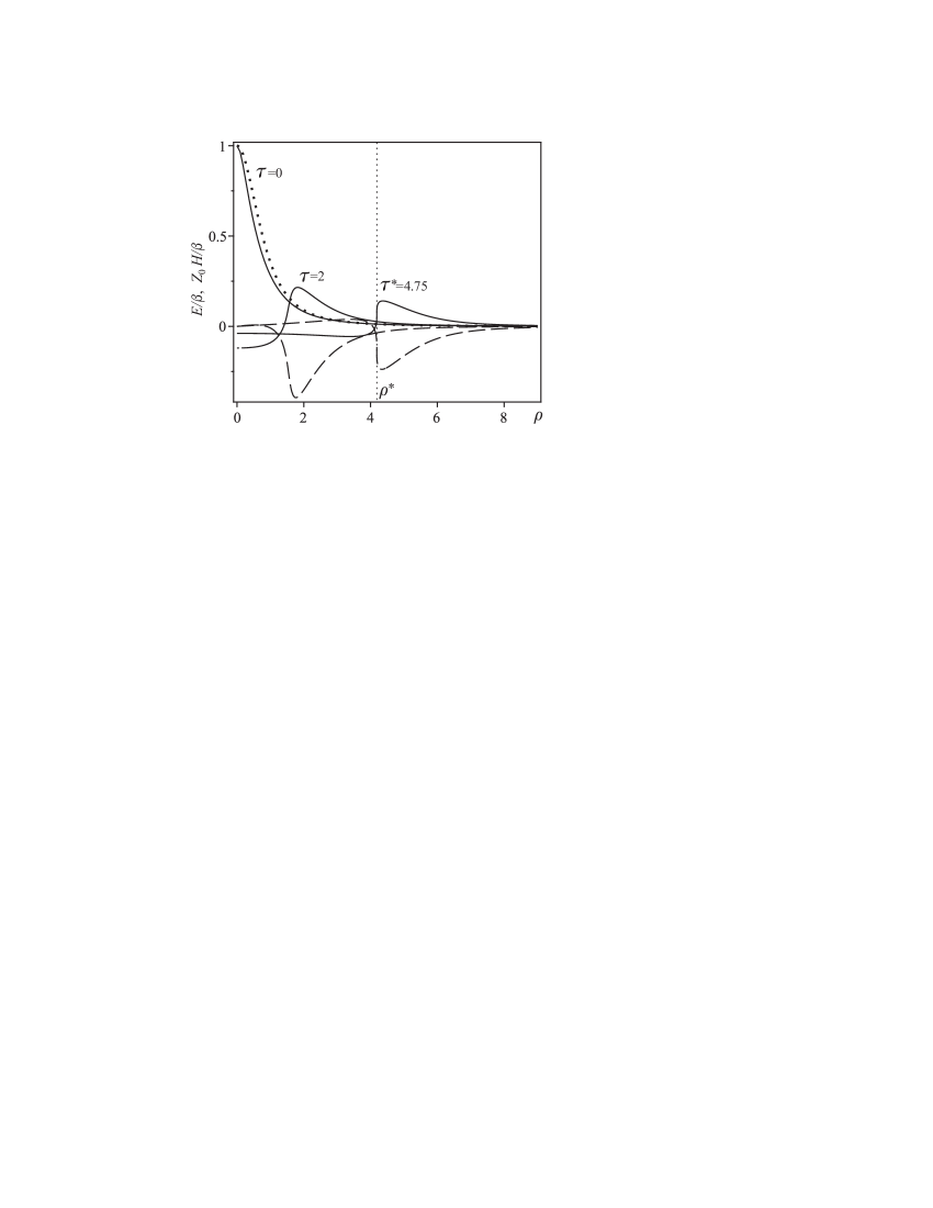
Figure 1: Radial distributions of the electric field (solid curves) and magnetic field (dashed curves) at various times $\tau$. The dotted curve corresponds to ${\cal E}(\rho,0)$ in Eqs. (13).

Fig. 1 shows results of numerical calculations of $E$ and $H$ by formulas (15) in the case where $\alpha\beta=1$ and $\varepsilon_{1}=2$. The electric and magnetic fields as functions of the coordinate $\rho$ are shown by the solid and dashed curves, respectively, at various times $\tau$. The dotted curve corresponds to the initial distribution (13) of the field $E$ in the auxiliary linear problem. It is evident that even for a sufficiently strong nonlinearity ($\alpha\beta=1$), the difference between the initial conditions (13) and (16) is small. Fig. 1 shows that the wave-profile part for which $E/\beta$ increases in the wave propagation direction becomes steeper with time, thereby exhibiting the so-called self-steepening. As a result, inflection of the wave profile occurs at a certain point $\rho=\rho^{*}$ at the time instant $\tau=\tau^{*}$. For $\tau>\tau^{*}$, three different values of both $E$ and $H$, which satisfy system (15), correspond to one value of $\rho$, so that the curves of $E$ and $H$ become ambiguous for a given $\tau$. Due to this fact, discontinuities of the wave components appear at the inflection point Landau et al. (1984), which corresponds to the formation of a cylindrical shock electromagnetic wave. Upon appearance of discontinuities, the solution in form (15) ceases to be suitable.

The appearance of discontinuities of electromagnetic quantities results from neglecting dispersion. Its influence leads to that the fields vary continuously under actual conditions. In this case, by a shock wave one should understand a sufficiently rapid variation in the field components on a certain moving interval. The thickness of this interval (shock front) sets so as to enable the polarization of the medium to switch from one value to the other.

Boundary value problem. Now consider a cavity resonator, which is a perfectly conducting circular cylinder of radius $a$ and height $L$. We assume that the $z$ axis is aligned with the cavity axis and the perfectly conducting end walls of the cavity are at $z=0$ and $z=L$. In the case where the cavity resonator is filled with a linear medium having the permittivity $\varepsilon=\epsilon_{0}\varepsilon_{1}={\rm const}$, $E_{0n0}$ (${\rm TM}_{0n0}$) modes can exist in the cavity. The $E_{z}$ and $H_{\phi}$ components, which are nonzero in these modes, are independent of $\phi$ and $z$, and are described by the solutions of system (10) with the boundary conditions

$$\left.E_{z}\right|_{r=a}\equiv{\cal E}(1,\tau)=0,\;\;|\left.E_{z}\right|_{r=0}|\equiv|{\cal E}(0,\tau)|<\infty.$$ (17)

Such solutions are well-known and their derivation can be found elsewhere Jackson (1998). Substituting the functions ${\cal E}$ and ${\cal H}$, which describe the $E_{0n0}$ modes, into Eqs. (12), we obtain the solution of nonlinear equations (1) in the form

$$E=A\,J_{0}(\kappa_{n}\,\rho\,e^{\alpha E/2})\,\cos(\kappa_{n}\theta),$$

$$H=-AZ^{-1}_{0}\varepsilon^{1/2}_{1}\,e^{\alpha E/2}J_{1}(\kappa_{n}\,\rho\,e^{\alpha E/2})\,\sin(\kappa_{n}\theta),$$ (18)

where $J_{m}$ is a Bessel function of the first kind of order $m$, $\kappa_{n}$ is the $n$th root of the equation $J_{0}(\kappa)=0$, and $A$ is an arbitrary amplitude factor. Note that the field $E=0$ satisfies the transcendental equations (18) for any $\tau$ if $\rho=r/a=1$. Therefore, the boundary conditions (17) remain valid for the implicit function $E(\rho,\tau)$ defined by Eqs. (18). Thus, formulas (18) yield an exact solution of the nonlinear boundary value problem for system (1) under conditions (17) and describe free electromagnetic oscillations in a cylindrical cavity filled with a nonlinear medium.

Implicit solutions $E$ and $H$ given by Eqs. (18) and corresponding to a certain index $n$ are periodic functions of time $t$ with period $T_{n}=2\pi/\omega_{n}$, where $\omega_{n}=\kappa_{n}(\epsilon_{0}\varepsilon_{1}\mu_{0})^{-1/2}a^{-1}$ is an eigenfrequency of the $E_{0n0}$ mode. Along with the fundamental frequency $\omega_{n}$ for each $n$, the Fourier time series expansions of the functions $E$ and $H$ also contain terms at the multiple frequencies $l\omega_{n}$, where $l$ is an integer. The contribution of harmonics with $l\geq 2$ determines the role of nonlinear effects which manifest themselves as deviations of the quantities $E$ and $H$ from their values corresponding to the $E_{0n0}$ mode in a cavity with $\varepsilon=\epsilon_{0}\varepsilon_{1}={\rm const}$ in the linear case ($\alpha=0$).

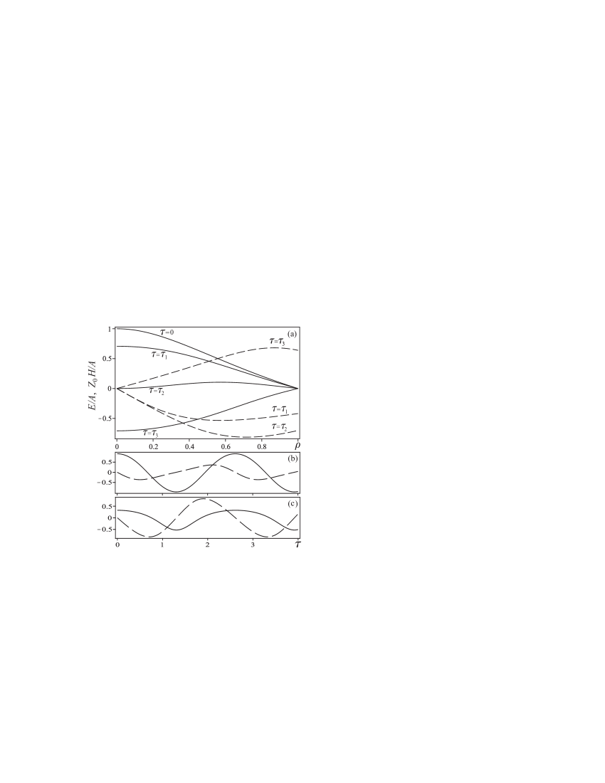
Figure 2: (a) Electric and magnetic fields as functions of $\rho$ (solid and dashed lines, respectively) in the $n=1$ mode at times $\tau_{1}=\pi/(4\kappa_{1})$, $\tau_{2}=\pi/(2\kappa_{1})$, and $\tau_{3}=5\pi/(4\kappa_{1})$. Oscillograms of the fields at (b) $\rho=0.2$ and (c) $\rho=0.7$.

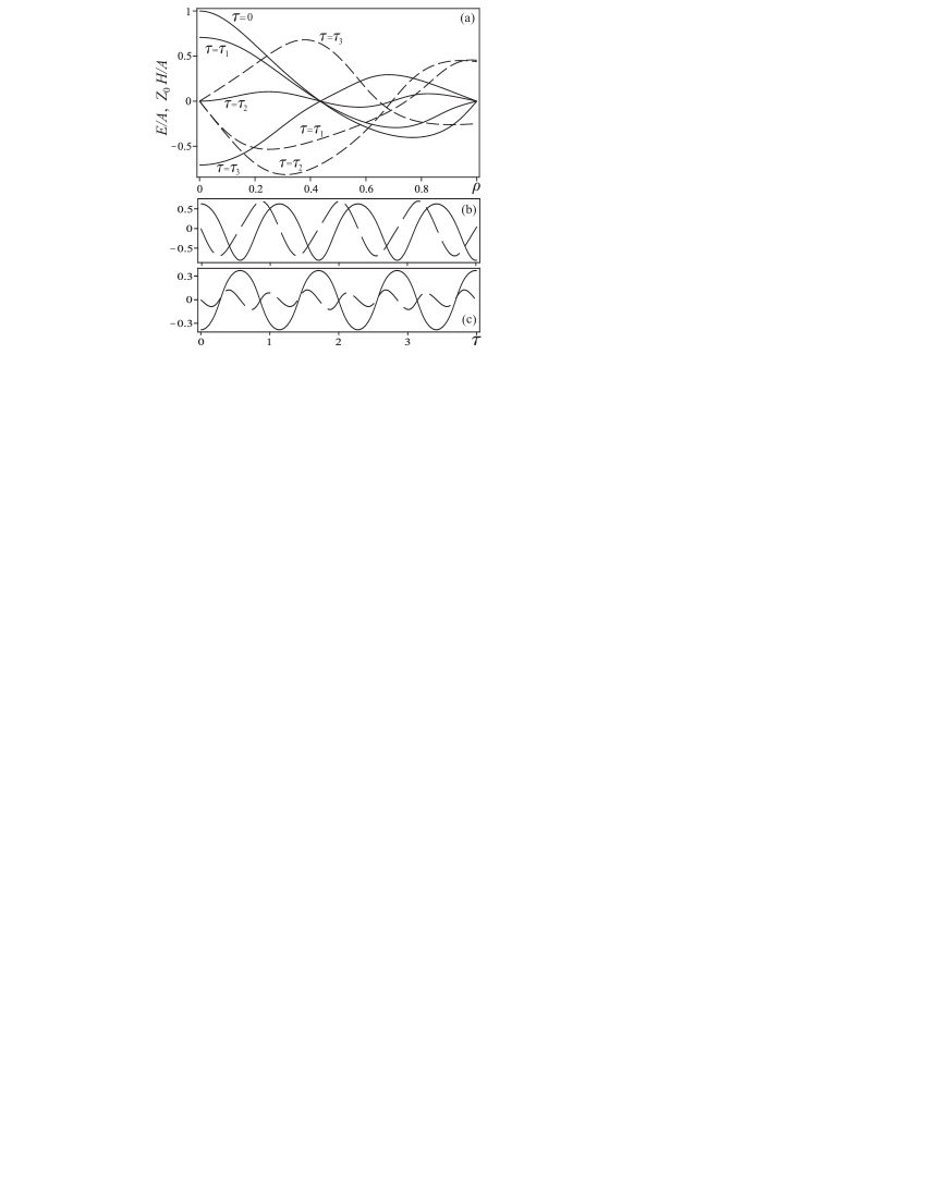
Figure 3: (a) The same as in Fig. 2(a), but for the $n=2$ mode at $\tau_{1}=\pi/(4\kappa_{2})$, $\tau_{2}=\pi/(2\kappa_{2})$, and $\tau_{3}=5\pi/(4\kappa_{2})$. Field oscillograms at (b) $\rho=0.2$ and (c) $\rho=0.7$.

Let us now turn to results of calculations of the quantities $E$ and $H$ by formulas (18). Fig. 2(a) shows snapshots of the normalized field components $E/A$ and $Z_{0}H/A$ in the lowest mode ($n=1$ and $\kappa_{1}\simeq 2.4$) as functions of $\rho$ at fixed instants of time $\tau$. Figs. 2(b) and 2(c) show the oscillograms of the field components at two points $\rho=0.2$ and $\rho=0.7$ for $n=1$. Similar curves for a mode with $n=2$ and $\kappa_{2}\simeq 5.5$ are presented in Fig. 3. Figs. 2 and 3 were plotted for $\alpha A=0.5$ and $\varepsilon_{1}=2$. The presented plots show that the nonlinear effects become more pronounced with increasing $n$ and depend significantly on the coordinate $\rho$, i.e., location of the observation point inside the cavity. For example, the field oscillograms in Fig. 3(b) are analogous to those in the linear case. However, in Fig. 3(c) we see that the field $E$ varies at the frequency $\omega_{2}$, while the field $H$, at the second harmonic $2\omega_{2}$. For the higher modes with $n>n^{*}$, where $n^{*}$ is an integer depending on the parameter $\alpha A$, the functions $E(\rho,\tau)$ and $H(\rho,\tau)$ determined by (18) become ambiguous in a certain domain of values of the variables $\rho$ and $\tau$. Since such behavior is not physically admissible, one should expect field discontinuities at the ambiguity points. The time dependences $E(\tau)$ and $H(\tau)$ can then be discontinuous (relaxation) oscillations, and the solutions (18) obtained without allowance for dispersion become inapplicable. However, it is important to emphasize that for weak nonlinearity ($|\alpha A|\ll 1$), the number $n^{*}$ is large (e.g., $n^{*}=9$ for $\alpha A=0.5$) and solutions (18) for $n<n^{*}$ are single-valued continuous functions of coordinates and time. Due to this fact, the exact solutions found seem to be of great practical interest and can be used for analysis of, e.g., ferroelectric resonators.

In conclusion, we note that the proposed method makes it to possible to easily generate various physically interesting solutions of nonlinear system (1), starting from the corresponding solutions of linear field equations. Therefore, this method has significant advantages over the direct numerical solution of that system.

This work was supported by the RFBR (project no. 09–02–00164-a) and the Russian Federal Program “Kadry.”

References

- Whitham (1974) G. B. Whitham, Linear and Nonlinear Waves (Wiley, New York, 1974).
- Ablowitz and Segur (1981) M. J. Ablowitz and H. Segur, Solitons and the Inverse Scattering Transform (SIAM, Philadelphia, 1981).
- Gaponov and Freidman (1959) A. V. Gaponov and G. I. Freidman, Sov. Phys. JETP 9, 675 (1959).
- Rosen (1965) G. Rosen, Phys. Rev. 139, A539 (1965).
- Polyanin and Zaitsev (2002) A. D. Polyanin and V. F. Zaitsev, Handbook of Nonlinear Partial Differential Equations (Chapman & Hall/CRC Press, Boca Raton, 2002).
- Fokas (2006) A. S. Fokas, Phys. Rev. Lett. 96, 190201 (2006).
- Franken and Ward (1963) P. A. Franken and J. F. Ward, Rev. Mod. Phys. 35, 23 (1963).
- Ivanov (1980) I. V. Ivanov, Sov. Phys. Usp. 23, 869 (1980).
- Belokopytov (1995) G. V. Belokopytov, Ferroelectrics 168, 69 (1995).
- Kudrin and E. Yu. Petrov (2010) A. V. Kudrin and E. Yu. Petrov, JETP 110, 537 (2010).
- Landau et al. (1984) L. D. Landau, E. M. Lifshitz, and L. P. Pitaevskii, Electrodynamics of Continuous Media (Pergamon, Oxford, 1984).
- Jackson (1998) J. D. Jackson, Classical Electrodynamics (Wiley, New York, 1998).