Cavity optomechanics with synthetic Landau levels of ultra cold Fermi gas

Bikash Padhi and Sankalpa Ghosh Department of Physics, Indian Institute of Technology Delhi, New Delhi-110016, India sankalpa@physics.iitd.ac.in
Abstract

Ultra cold fermionic atoms placed in a synthetic magnetic field arrange themselves in Landau levels. We theoretically study the optomechanical interaction between the light field and collective excitations of such fermionic atoms in synthetic magnetic field by placing them in side a Fabry Perot cavity. We derive the effective hamiltonian for particle hole excitations from a filled Landau level using a bosonization technique and obtain an expression for the cavity transmission spectrum. Using this we show that the cavity transmission spectrum demonstrates cold atom analogue of Subnikov de Hass oscillation in electronic condensed matter systems. We discuss the experimental consequences for this oscillation for such system and the related optical bistability.

pacs:
42.50.Pq, 03.75.Ss, 73.43.-f

By allowing an ultracold atomic ensemble to interact with a selected mode of a high finesse cavity it is possible to probe the quantum many body state of such an ultra cold atomic system. The resulting cavity-optomechanics or cavity quantum electrodynamics with ultra cold atoms in recent times witnessed significant development review1 . The experimental successes include the coupling of collective density excitation of a ultra cold bosonic condensate with a single cavity mode and observing the coupled dynamics through cavity transmission Eslng , a strongly coupled cavity mode with a highly localized ultra cold atomic condensate trapped inside a single antinode of a cavity field Colombe , demonstration of strong ultracold atom-cavity coupling induced optical non-linearity even at low photon density Kurn and selected atom-photn coupling of single atomic ensemble in a multi-ensemble system Kurn1 to name a few.

In another development, there has been significant experimental and theoretical progress in studying the effect of optically induced artificial or synthetic gauge field artificial on such neutral atoms, making it a playground for quantum simulation of phenomena that occur when electronic condensed matter system is placed in a real magnetic field. The experimental achievements in this direction include the observation of vortices, Abrikosov vortex lattice in trapped ultra cold atomic superfluid initially by achieving the synthetic magnetic field through the rotation of the trapvortices , and later by Raman laser induced spatially varying coupling of the hyperfine states of such ultra cold atoms synthetic . More recent development in this direction includes the creation of optical flux lattices opticalflux , realization of spin-orbit coupling for such neutral ultracold bosonic spinorbitB and fermionic atoms spinorbitF with the possibility of creating ultra cold atomic analogues of topological condensed matter phases.

This letter aims to combine these two developments by considering a system of such ultra cold atoms trapped inside a high finesse Fabry Perot cavity interacting with 
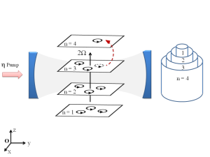
a single cavity mode ( see Fig. 1 ), additionally, in the presence of a synthetic magnetic field. Specifically we consider the case of ultra cold fermionic atoms Jin1 in a synthetic magnetic field Ho ; Lewen such that a set of Landau levels can be filled according to Pauli principle. We consider the coupling between the bosonic particle-hole like excitations from such filled Landau levels of fermionic atoms with the cavity mode. We find that the atom-photon coupling explicitly shows Landau level degeneracy, and has finite discontinuities at certain values of artificial magnetic field strength that resembles the well known Subnokov de Haas oscillation SdH in condensed matter system. The cavity transmission spectrum shows optical bistability, a hall mark of optical non-linearity in such cavity system Meystre , but now the features of the bistable curve also reveals the Landau level structure. Our results suggest that cavity optomechanics with such atomic Landau levels can be a powerful probe for ultra cold atoms in synthetic gauge field.

We consider two dimensional system of N ultracold neutral fermionic two-level atoms each of mass $M$ subjected to a synthetic magnetic field synthetic ; Ho ; Lewen ; review , placed inside Fabry-P${\acute{e}}$rot cavity of area $\mathcal{A}$ which is driven at the rate of ${\eta}$ by a pump laser of frequency ${\omega}_{p}$ and wave vector $\boldsymbol{K}=(K_{x},K_{y})$. The atoms have transition frequency $\omega_{a}$, and interact strongly with a single standing wave empty cavity mode of frequency $\omega_{c}$.

Refer to caption
Figure 1: Schematic diagram of the system considered is shown. The concentric cylindrical surfaces represent the fermi surfaces that correspond to Landau levels of (LL) of fermionic atoms inside the cavity with LL quantum number $n$. The particle hole excitation from the last filled Landau level is also also shown.

We take the artificial magnetic field as $2\Omega\hat{z}$. We also ignore the effective trap potential assuming it is shallow enough in the bulk. The resulting single particle hamiltonian is analogous to Landau problem of a charged particle in a transverse magnetic field ( for details see suppli1 ) that can be written as.

$$H_{L}=\frac{1}{2M}{\bf\Pi}^{2},$$ (1)

where ${\bf\Pi}={\bf p}-M{\bf A}$ is the kinetic momentum, with the effective vector potential ${\bf A}={\bf\Omega\times r}$ in symmetric gauge. The eigenstates of this Hamiltonian are Landau levels with effective cyclotron frequency $\omega_{0}=2\Omega$, and eigen-energies $E_{n,m}=2\hbar\Omega(n+1/2)$. The effective magnetic length in this problem is $l_{0}=\sqrt{\hbar/2M\Omega}$.

If the pump laser frequency $\omega_{p}$ is far detuned from the atomic transition frequency $\omega_{a}$, the excited electronic state of the two level atoms can be adiabatically eliminated. It is assumed that such atoms interact dispersively with the cavity field, taken to be single mode. In the dipole and rotating wave approximation, we get the effective system Hamiltonian( details in suppli1 )

$\displaystyle\hat{H}_{eff}$ $\displaystyle=$ $\displaystyle\hat{H}_{L}+\hat{H}_{I}+\hat{H}_{C},\text{with}$ (2)
$\displaystyle\hat{H}_{L}$ $\displaystyle=$ $\displaystyle{{\int}d^{2}{\bf r}}{\hat{\Psi}^{\dagger}(\boldsymbol{r})}\Big{[}{\bf\hat{\Pi}}^{2}/2M\Big{]}{\hat{\Psi}(\boldsymbol{r})},$ (3)
$\displaystyle\hat{H}_{I}$ $\displaystyle=$ $\displaystyle{{\int}d^{2}{\bf r}}{\hat{\Psi}^{\dagger}(\boldsymbol{r})}\Big{[}\hbar U_{0}cos^{2}({\bf K}.{\bf r})\hat{a}^{\dagger}\hat{a}\Big{]}{\hat{\Psi}(\boldsymbol{r})},$ (4)
$\displaystyle\hat{H}_{C}$ $\displaystyle=$ ℏ​Δc​a^†​a^βˆ’Δ±β€‹β„β€‹Ξ·β€‹(a^βˆ’a^†).Planck-constant-over-2-pisubscriptΔ𝑐superscript^π‘Žβ€ ^π‘Žitalic-Δ±Planck-constant-over-2-piπœ‚^π‘Žsuperscript^π‘Žβ€ \displaystyle{\hbar{\Delta_{c}}}\hat{a}^{\dagger}\hat{a}-{\imath}{\hbar}{\eta}(\hat{a}-\hat{a}^{\dagger}). (5)

Here $U_{0}=g_{0}^{2}/\Delta_{a}$ is the effective light-matter coupling constant with $g_{0}$ is single photon Rabi frequency, $\Delta_{a}=\omega_{p}-\omega_{a}$. Here $\hat{H}_{L}$ is the atomic Hamiltonian in the synthetic magnetic field, $\hat{H}_{C}$ captures the dynamics of the cavity photons with $\Delta_{c}=\omega_{c}-\omega_{p}$. $\hat{H}_{I}$ is the term that describes interaction between atom and the cavity mode. The atomic field operator in the Landau level basis (symmetric gauge) is given as

$\displaystyle\hat{\Psi}(\boldsymbol{r})$ $\displaystyle=$ $\displaystyle\sum\limits_{m,n}\hat{c}_{n,m}\langle{\bf r}|n,m\rangle=\sum\limits_{m,n}\frac{e^{-|z|^{2}/4l_{0}^{2}}}{\sqrt{2\pi l_{0}^{2}}}G_{m+n,n}(iz/l_{0})\hat{c}_{n,m}$ (6)
with,{c^n,m†,c^nβ€²,m′†}withsuperscriptsubscript^π‘π‘›π‘šβ€ subscriptsuperscript^𝑐†superscript𝑛′superscriptπ‘šβ€²\displaystyle\text{with},\{\hat{c}_{n,m}^{\dagger},\hat{c}^{\dagger}_{n^{\prime},m^{\prime}}\} $\displaystyle=$ $\displaystyle\{\hat{c}_{n,m},\hat{c}_{n^{\prime},m^{\prime}}\}=0$
{c^n,m†,c^nβ€²,mβ€²}subscriptsuperscript^π‘β€ π‘›π‘šsubscript^𝑐superscript𝑛′superscriptπ‘šβ€²\displaystyle\{\hat{c}^{\dagger}_{n,m},\hat{c}_{n^{\prime},m^{\prime}}\} $\displaystyle=$ $\displaystyle\delta_{n,n^{\prime}}\delta_{m,m^{\prime}},$ (7)

with $z=x+\imath y$. $|n,m\rangle$ is the Landau-eigenket. $\langle{\bf r}|n,m\rangle$ is the symmetric-gauge wavefunction. $\frac{e^{-|z|^{2}/4l_{0}^{2}}}{\sqrt{2\pi l_{0}^{2}}}G_{n+m,m}(iz/l_{0})$ are two dimensional harmonic oscillator wavefunction whose properties are given in suppli1 .

c^n,m†superscriptsubscript^π‘π‘›π‘šβ€ \hat{c}_{n,m}^{\dagger} is the fermionic creation operator that creates the state $|n,m\rangle$, namely a fermion in the $n^{th}$ Landau level (LL), with the guiding center $m$ obeying (7) with $n=0,1,2...,\nu-1$ and $m=0,1,2,...,N_{\phi}-1$. $\nu=N/N_{\phi}$ is called the filling factor where $N_{\phi}=\mathcal{A}/(2\pi l_{0}^{2})$ is the degeneracy of each Landau level. The atomic Hamiltonian ($\hat{H}_{L}$) can be diagonalized in the Landau level basis yielding H^L=ℏ​ω0β€‹βˆ‘m,n=0∞(n+12)​c^n,m†​c^n,m.subscript^𝐻𝐿Planck-constant-over-2-pisubscriptπœ”0superscriptsubscriptπ‘šπ‘›0𝑛12superscriptsubscript^π‘π‘›π‘šβ€ subscript^π‘π‘›π‘š\hat{H}_{L}=\hbar{\omega}_{0}\sum\limits_{m,n=0}^{\infty}(n+\frac{1}{2})\hat{c}_{n,m}^{\dagger}\hat{c}_{n,m}. Using $4cos^{2}({\bf K.r})=2+2cos(2{\bf K.r})=2+e^{-\imath 2{\bf K.r}}+e^{\imath 2{\bf K.r}}$, $\hat{H}_{I}$) in the Landau basis can be written as

$\displaystyle\hat{H}_{I}$ $\displaystyle=$ $\displaystyle\frac{\hbar U_{0}}{4}\Big{\{}\hat{N}+\sum\limits\hat{c}_{n^{\prime},m^{\prime}}^{\dagger}\hat{c}_{n,m}e^{-2(|K|l_{0})^{2}}\Big{(}G_{n^{\prime},n}(2K^{*}l_{0})G_{m^{\prime},m}(2Kl_{0})+$ (8)
$\displaystyle G_{n^{\prime},n}(-2K^{*}l_{0})G_{m^{\prime},m}(-2Kl_{0})\Big{)}\Big{\}}\hat{a}^{\dagger}\hat{a}$

where $K=K_{x}+\imath K_{y}$, $K^{*}=K_{x}-\imath K_{y}$, $|K|^{2}=K_{x}^{2}+K_{y}^{2}$, and the summations are done over all available $n,n^{\prime},m,m^{\prime}$. If we assume that the interaction time between the cavity and ultra cold fermions is much shorter than any time scale associated with the reorganization of the atomic ground state in presence of the standing wave inside the cavity, the role of the interaction hamiltonian (IV.4) is restricted to transfer momentum $\pm 2|K|$ to the particle-hole excitation above the Fermi level.

By looking at the cavity transmission spectrum we are interested in studying such low energy excitations above an integer number of filled Landau level. Such particle-hole excitations are bosonic in nature and known as magnetic exciton in the literature of quantum hall systems Halperin . In the absence of atom-photon interaction the ground state of our system is a direct product state of photonic vacuum and excitonic vacuum, obtained by completely filling the first $\nu$ Landau levels of each guiding center

|G​S⟩=∏m=0NΟ•βˆ’1∏n=0Ξ½βˆ’1cn,m†​|0⟩.ket𝐺𝑆superscriptsubscriptproductπ‘š0subscript𝑁italic-Ο•1superscriptsubscriptproduct𝑛0𝜈1superscriptsubscriptπ‘π‘›π‘šβ€ ket0|GS\rangle=\prod\limits_{m=0}^{N_{\phi}-1}\prod\limits_{n=0}^{\nu-1}c_{n,m}^{\dagger}|0\rangle. (9)

These inter Landau level excitations only involve the change in the Landau level index, they can be studied using the language of bosonization Calderia by introducing bosonic operator

b^p†​(𝐀)=1p​Nϕ​Jp2​(k​RΞ½)​eβˆ’(l0​|k|)2/2β€‹βˆ‘n=0βˆžβˆ‘m,mβ€²=0∞c^n+p,m′†​c^n,m​(Gn+p,n​(l0​kβˆ—)​Gmβ€²,m​(l0​k)).subscriptsuperscript^𝑏†𝑝𝐀1𝑝subscript𝑁italic-Ο•superscriptsubscript𝐽𝑝2π‘˜subscriptπ‘…πœˆsuperscript𝑒superscriptsubscript𝑙0π‘˜22superscriptsubscript𝑛0superscriptsubscriptπ‘šsuperscriptπ‘šβ€²0superscriptsubscript^𝑐𝑛𝑝superscriptπ‘šβ€²β€ subscript^π‘π‘›π‘šsubscript𝐺𝑛𝑝𝑛subscript𝑙0superscriptπ‘˜subscript𝐺superscriptπ‘šβ€²π‘šsubscript𝑙0π‘˜\hat{b}^{\dagger}_{p}({\bf k})=\frac{1}{\sqrt{pN_{\phi}J_{p}^{2}(kR_{\nu})}}e^{-(l_{0}|k|)^{2}/2}\sum\limits_{n=0}^{\infty}\sum\limits_{m,m^{\prime}=0}^{\infty}\hat{c}_{n+p,m^{\prime}}^{\dagger}\hat{c}_{n,m}\Big{(}G_{n+p,n}(l_{0}k^{*})G_{m^{\prime},m}(l_{0}k)\Big{)}. (10)

This operator creates a bosonic particle-hole excitation by shifting an atom from $n$-th LL to the $n+p$-th LL where $J_{p}$ is the Bessel function of first kind , $R_{\nu}=\sqrt{2\nu}l_{0}$, and obeys

[b^p​(𝐀),b^q​(𝐀′)]=[b^p†​(𝐀),b^q†​(𝐀′)]=0subscript^𝑏𝑝𝐀subscript^π‘π‘žsuperscript𝐀′subscriptsuperscript^𝑏†𝑝𝐀subscriptsuperscript^π‘β€ π‘žsuperscript𝐀′0[\hat{b}_{p}({\bf k}),\hat{b}_{q}({\bf k^{\prime}})]=[\hat{b}^{\dagger}_{p}({\bf k}),\hat{b}^{\dagger}_{q}({\bf k^{\prime}})]=0
[b^p​(𝐀),b^q†​(𝐀′)]=δ​(π€βˆ’π€β€²)​δp,q.subscript^𝑏𝑝𝐀subscriptsuperscript^π‘β€ π‘žsuperscript𝐀′𝛿𝐀superscript𝐀′subscriptπ›Ώπ‘π‘ž[\hat{b}_{p}({\bf k}),\hat{b}^{\dagger}_{q}({\bf k^{\prime}})]=\delta({\bf k}-{\bf k^{\prime}})\delta_{p,q}. (11)

Using the commutators of the bosonic opertaor (11) the bosonized version of the Landau level hamiltonian (3) of ultra cold fermions can be written as

$$\hat{H}_{L}=\hbar\sum\limits_{p=1}^{\infty}\sum\limits_{\bf k}p\omega_{0}b_{p}^{\dagger}({\bf k})b_{p}({\bf k}).$$ (12)

The atom-photon interaction (IV.4), can similarly be rewritten in terms of the bosonic operator (10) as

H^I=ℏ​U04​N^​a^†​a^+ℏ​U04β€‹βˆ‘p=1∞Nϕ​p​Jp2​(2​K​RΞ½)​(b^p†​(2β€‹πŠ)+b^p​(2β€‹πŠ))​a^†​a^.subscript^𝐻𝐼Planck-constant-over-2-pisubscriptπ‘ˆ04^𝑁superscript^π‘Žβ€ ^π‘ŽPlanck-constant-over-2-pisubscriptπ‘ˆ04superscriptsubscript𝑝1subscript𝑁italic-ϕ𝑝superscriptsubscript𝐽𝑝22𝐾subscriptπ‘…πœˆsuperscriptsubscript^𝑏𝑝†2𝐊subscript^𝑏𝑝2𝐊superscript^π‘Žβ€ ^π‘Ž\hat{H}_{I}=\frac{\hbar U_{0}}{4}\hat{N}\hat{a}^{\dagger}\hat{a}+\frac{\hbar U_{0}}{4}\sum\limits_{p=1}^{\infty}\sqrt{N_{\phi}pJ_{p}^{2}(2KR_{\nu})}\Big{(}\hat{b}_{p}^{\dagger}(2{\bf K})+\hat{b}_{p}(2{\bf K})\Big{)}\hat{a}^{\dagger}\hat{a}. (13)

The derivation of the hamiltonian (12), and (13) from (IV.4) is given in the supplementary information suppli1 . The bosonized effective Hamiltonian (2) of the atom-photon system thus becomes

$\displaystyle\hat{H}_{eff}$ $\displaystyle=$ β„β€‹βˆ‘p=1∞{βˆ‘π€p​ω0​b^p†​(𝐀)​b^p​(𝐀)+Ξ΄pν​p​(b^p†​(2β€‹πŠ)+b^p​(2β€‹πŠ))​a^†​a^}Planck-constant-over-2-pisuperscriptsubscript𝑝1subscript𝐀𝑝subscriptπœ”0superscriptsubscript^𝑏𝑝†𝐀subscript^𝑏𝑝𝐀subscriptsuperscriptπ›Ώπœˆπ‘π‘superscriptsubscript^𝑏𝑝†2𝐊subscript^𝑏𝑝2𝐊superscript^π‘Žβ€ ^π‘Ž\displaystyle\hbar\sum\limits_{p=1}^{\infty}\Big{\{}\sum\limits_{\bf k}p\omega_{0}\hat{b}_{p}^{\dagger}({\bf k})\hat{b}_{p}({\bf k})+\delta^{\nu}_{p}\sqrt{p}\Big{(}\hat{b}_{p}^{\dagger}(2{\bf K})+\hat{b}_{p}(2{\bf K})\Big{)}\hat{a}^{\dagger}\hat{a}\Big{\}} (14)
+ℏ​Δ​a^†​a^βˆ’Δ±β€‹β„β€‹Ξ·β€‹(a^βˆ’a^†),Planck-constant-over-2-piΞ”superscript^π‘Žβ€ ^π‘Žitalic-Δ±Planck-constant-over-2-piπœ‚^π‘Žsuperscript^π‘Žβ€ \displaystyle+{\hbar{\Delta}}\hat{a}^{\dagger}\hat{a}-{\imath}{\hbar}{\eta}(\hat{a}-\hat{a}^{\dagger}),
$\displaystyle\delta^{\nu}_{p}$ $\displaystyle=$ $\displaystyle\frac{U_{0}}{4}\sqrt{N_{\phi}J_{p}^{2}(2KR_{\nu})}.$ (15)

The above hamiltonian is one of the central result of this paper. Here the operator $\hat{N}$ is replaced with its steady-state expectation value, subsequently the term N​ℏ​U02​a^†​a𝑁Planck-constant-over-2-pisubscriptπ‘ˆ02superscript^π‘Žβ€ π‘Ž\frac{N\hbar U_{0}}{2}\hat{a}^{\dagger}a is incorporated into ℏ​Δc​a†​aPlanck-constant-over-2-pisubscriptΔ𝑐superscriptπ‘Žβ€ π‘Ž{\hbar{\Delta_{c}}}a^{\dagger}a of $H_{C}$ to get the effective cavity detuning $\Delta=\omega_{c}-\omega_{p}+\frac{NU_{0}}{2}$.

The Ξ΄pΞ½subscriptsuperscriptπ›Ώπœˆπ‘\delta^{\nu}_{p} is the atom-photon coupling constant that couples the excited levels with the photon field. 
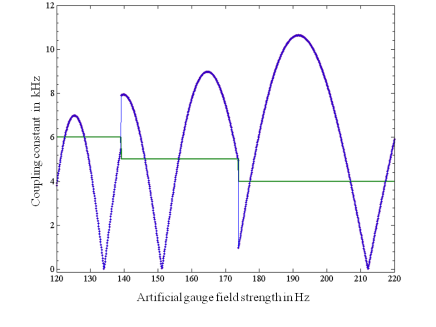
Fig. (2) depicts its variation with the field strength when an atom gets excited from the filled LL to the next unoccupied LL. For that purpose we choose experimentally achievable parameters, Ξ»=500​n​m​(K≃107​mβˆ’1),π’œβ‰ƒ(30​μ​m)2,ΞΊ=2​π​M​H​zformulae-sequenceπœ†500π‘›π‘šsimilar-to-or-equals𝐾superscript107superscriptπ‘š1formulae-sequencesimilar-to-or-equalsπ’œsuperscript30πœ‡π‘š2πœ…2πœ‹π‘€π»π‘§\lambda=500nm(K\simeq 10^{7}m^{-1}),\mathcal{A}\simeq(30\mu m)^{2},\kappa=2\pi MHz, atomic mass M=1.5Γ—10βˆ’25​k​g,N=2000,g0=2​π×10​M​H​z,formulae-sequence𝑀1.5superscript1025π‘˜π‘”formulae-sequence𝑁2000subscript𝑔02πœ‹10𝑀𝐻𝑧M=1.5\times 10^{-25}kg,N=2000,g_{0}=2\pi\times 10MHz, pump-atom detuning Ο‰pβˆ’Ο‰a=2​π×50​G​H​zsubscriptπœ”π‘subscriptπœ”π‘Ž2πœ‹50𝐺𝐻𝑧\omega_{p}-\omega_{a}=2\pi\times 50GHz. It lineary depends on atom-photon coupling constant U0subscriptπ‘ˆ0U_{0} and is enhanced by the Landau level degenracy NΟ•subscript𝑁italic-Ο•{\sqrt{N_{\phi}}}, different as compared to the case of ordinary fermions Meystre and akin to the scaling of the atom-photon coupling constant by N𝑁\sqrt{N} for a N-boson condensate Eslng ; Colombe . In Fig. (2), with increasing ΩΩ\Omega, the coupling constant oscillates along with jump discontinuities. This is the usual Subnikov de Hass effect SdH , now occuring for a synthetic magnetic field when the fermi level makes a jump to the previous level at some increased value of the field.

The other important feature, the oscillatory behaviour of $\delta^{\nu}_{p}$ can be attributed to the length scales associated with the current problem. In presence of synthetic gauge field the cyclotron radius of the ultracold atoms ($l_{0}\sim 200-800nm$) is comparable with the wavelength of the probing photon ($\lambda\sim 600nm$). With increase in field strength the cyclotron radius decreases and the number of wavelengths that fits within this radius also changes, leading to the oscillatory behavior of the atom-photon coupling strength as a function of the field strength. In comparison, in the corresponding electronic problem the electron cyclotron radius is much smaller ($l_{0}\sim 20nm$ ) so the incident photon can not actually see the individual cyclotron orbit, making such oscillation hard to be observed in electronic LL spectroscopy spec1 ; spec2 .

Refer to caption
Figure 2: Variation of coupling constant (for p=1) with synthetic field strength. The green colored steps in the background correspond to the corresponding first empty LL, $\nu$ = 6,5,4.

.

The oscillation of the coupling constant as a function of the strength of the synthetic gauge field can be obtained from the steady state cavity transmission spectrum, an experimentally measurable quantity. The hamiltonian (14) represents a coupled system of particle-hole excitations ( magnetic exciton) and photons. The steady state solution of Heisenberg equations for operators associated with the dynamics of exciton and photon yields the cavity transmission spectrum. To this purpose we introduce phase space quadrature variables

$$\hat{X}_{L}=(\hat{b}_{p}^{\dagger}(2{\bf K})+\hat{b}_{p}({2\bf K}))/\sqrt{2};\hat{P}_{L}=\imath(\hat{b}_{p}^{\dagger}(2{\bf K})-\hat{b}_{p}(2{\bf K}))/\sqrt{2}.$$

which obey standard commutator $[\hat{X}_{L},\hat{P}_{L}]=\imath$. The resulting Heisenberg equations are

$\displaystyle\frac{d\hat{X}_{L}}{dt}$ $\displaystyle=$ p​ω0​P^L,d​P^Ld​t=βˆ’p​ω0​X^Lβˆ’Ξ΄pν​2​p​a^†​a^,𝑝subscriptπœ”0subscript^𝑃𝐿𝑑subscript^𝑃𝐿𝑑𝑑𝑝subscriptπœ”0subscript^𝑋𝐿subscriptsuperscriptπ›Ώπœˆπ‘2𝑝superscript^π‘Žβ€ ^π‘Ž\displaystyle p\omega_{0}\hat{P}_{L},\quad\quad\frac{d\hat{P}_{L}}{dt}=-p\omega_{0}\hat{X}_{L}-\delta^{\nu}_{p}\sqrt{2p}\hat{a}^{\dagger}\hat{a},
$\displaystyle\frac{d\hat{a}}{dt}$ $\displaystyle=$ $\displaystyle-\imath\sum\limits_{p=1}^{\infty}\delta^{\nu}_{p}\sqrt{2p}\hat{X}_{L}\hat{a}-\imath\Delta\hat{a}+\eta-\kappa\hat{a}+\sqrt{2\kappa}\hat{a}_{in}.$ (16)

Here $\kappa$ is the cavity decay rate and $\hat{a}_{in}$ denotes a Markovian noise operatornoise with zero mean, and correlation ⟨a^i​n†​(t)​a^i​n​(tβ€²)⟩=2​κ​δ​(tβˆ’tβ€²),delimited-⟨⟩superscriptsubscript^π‘Žπ‘–π‘›β€ π‘‘subscript^π‘Žπ‘–π‘›superscript𝑑′2πœ…π›Ώπ‘‘superscript𝑑′\langle\hat{a}_{in}^{\dagger}(t)\hat{a}_{in}(t^{\prime})\rangle=2\kappa\delta(t-t^{\prime}), and $\langle\hat{a}_{in}(t)\hat{a}_{in}(t^{\prime})\rangle=0$, so can be dropped for steady state analysis. The steady state solutions are given by

$\displaystyle\hat{P}_{L}^{(s)}=0,\quad$ X^L(s)=βˆ’Ξ΄pν​2​pp​ω0​a^†(s)​a^(s),superscriptsubscript^𝑋𝐿𝑠subscriptsuperscriptπ›Ώπœˆπ‘2𝑝𝑝subscriptπœ”0superscript^π‘Žβ€ absent𝑠superscript^π‘Žπ‘ \displaystyle\hat{X}_{L}^{(s)}=-\frac{\delta^{\nu}_{p}\sqrt{2p}}{p\omega_{0}}\hat{a}^{{\dagger}(s)}\hat{a}^{(s)},\quad
a^(s)superscript^π‘Žπ‘ \displaystyle\hat{a}^{(s)} $\displaystyle=$ Ξ·ΞΊ+ı​(Ξ”βˆ’Sν​a^†(s)​a^(s)),withπœ‚πœ…italic-Δ±Ξ”subscriptπ‘†πœˆsuperscript^π‘Žβ€ absent𝑠superscript^π‘Žπ‘ with\displaystyle\frac{\eta}{\kappa+\imath(\Delta-S_{\nu}\hat{a}^{{\dagger}(s)}\hat{a}^{(s)})},\text{with}
$\displaystyle S_{\nu}$ $\displaystyle=$ $\displaystyle\frac{2}{\omega_{0}}\sum\limits_{p=1}^{\infty}(\delta^{\nu}_{p})^{2}=\frac{U_{0}^{2}\mathcal{A}M}{32\pi\hbar}(1-J_{0}^{2}(2KR_{\nu})).$ (17)

Therefore steady state inter cavity photon number is

n^p​h=a^†(s)​a^(s)=Ξ·2ΞΊ2+(Ξ”βˆ’Sν​n^p​h)2.subscript^π‘›π‘β„Žsuperscript^π‘Žβ€ absent𝑠superscript^π‘Žπ‘ superscriptπœ‚2superscriptπœ…2superscriptΞ”subscriptπ‘†πœˆsubscript^π‘›π‘β„Ž2\hat{n}_{ph}=\hat{a}^{{\dagger}(s)}\hat{a}^{(s)}=\frac{\eta^{2}}{\kappa^{2}+(\Delta-S_{\nu}\hat{n}_{ph})^{2}}. (18)

The cavity transmission spectrum is given by its expectation value that follows

$\displaystyle S_{\nu}^{2}n_{ph}^{3}-2S_{\nu}\Delta n_{ph}^{2}+(\kappa^{2}+\Delta^{2})n_{ph}=\eta^{2}.$ (19)
Refer to caption
Refer to caption
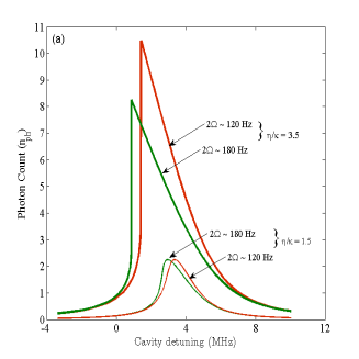
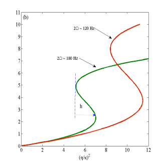
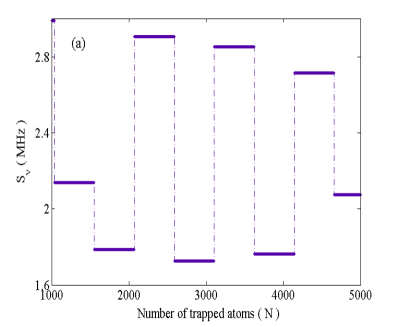
Figure 3: Steady-state interactivity photon number as a function of (a) pump cavity detuning for a set of synthetic field and $\eta/\kappa$; (b) pump rate for the same set of synthetic fields and cavity detuning $\Delta=2\pi\times$ 2.5 MHz.

Such non-linear cubic equation is characteristic of optical multistability Eslng ; Kurn . Figure 3 shows the behavior of steady-state mean photon number as a function of pump rate, and $\Delta$. To understand this multistability we study the fluctuation around the steady state, through a linear stability analysis. To that purpose, we write np​h=np​hs+δ​np​hsubscriptπ‘›π‘β„Žsuperscriptsubscriptπ‘›π‘β„Žπ‘ π›Ώsubscriptπ‘›π‘β„Žn_{ph}=n_{ph}^{s}+\delta n_{ph} in Eq. (19) where np​hssuperscriptsubscriptπ‘›π‘β„Žπ‘ n_{ph}^{s} corresponds to the steady state inter cavity photon number plotted in Fig. 3 (b). Then only the terms linear in $\delta n_{ph}$ are kept in the resulting equation, and the steady state solution (19) is substituted in it to get

(3​SΞ½2​(np​hs)2βˆ’4​Sν​Δ​np​hs+(ΞΊ2+Ξ”2))​δ​np​h=0.3superscriptsubscriptπ‘†πœˆ2superscriptsuperscriptsubscriptπ‘›π‘β„Žπ‘ 24subscriptπ‘†πœˆΞ”superscriptsubscriptπ‘›π‘β„Žπ‘ superscriptπœ…2superscriptΞ”2𝛿subscriptπ‘›π‘β„Ž0\left(3S_{\nu}^{2}(n_{ph}^{s})^{2}-4S_{\nu}\Delta n_{ph}^{s}+(\kappa^{2}+\Delta^{2})\right)\delta n_{ph}=0. (20)

The solution of this equation defines the upper and lower bound of the unstable regime as the turning points of the plot in Fig. 3 (b). In the region between these two turning points, the inter cavity photon number is a decreasing function of the cavity parameter $(\frac{\eta}{\kappa})^{2}$ and corresponds to the unstable solution MeystreB ; Gibbs .

A more formal way of doing the linear stability analysis is through the Heisenberg equation of motion of the operators, namely setting $\mathcal{O}(t)=\mathcal{O}^{(s)}+\delta\mathcal{O}(t)$. However for the current problem $\mathcal{O}(t)=[\hat{X}_{L}(t)^{p=1},\hat{P}_{L}(t)^{p=1},\hat{X}_{L}(t)^{p=2},\hat{P}_{L}(t)^{p=2},\cdots,\hat{X}(t),\hat{P}(t)]^{T},$ with X^=(a^†+a^)/2,P^=ı​(a^β€ βˆ’a^)/2formulae-sequence^𝑋superscript^π‘Žβ€ ^π‘Ž2^𝑃italic-Δ±superscript^π‘Žβ€ ^π‘Ž2\hat{X}=(\hat{a}^{\dagger}+\hat{a})/\sqrt{2},\hat{P}=\imath(\hat{a}^{\dagger}-\hat{a})/\sqrt{2} being the cavity quadratures. The linear stability analysis gets contribution from all $p$Β s and the resulting stability matrix is infinite dimensional and cannot be handled in the same way like one in the absence of such synthetic gauge field Meystre . A more detailed discussion on this issue is given in the supplimentary information suppli1 .
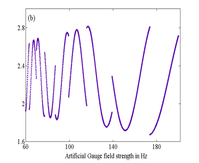
Refer to caption
Refer to caption
Figure 4: Variation of $S_{\nu}$ with (a) number of trapped atoms and (b) gauge field strength.

The distance between the two turning points of the bistability curve in Fig. 3(b) is calculated to be

$$h(S_{\nu})=\frac{4(\Delta^{2}-3\kappa^{2})^{3/2}}{27S_{\nu}}.$$ (21)

An experimentally obtained cavity spectrum Eslng ; Colombe ; Kurn can be used to extract the corresponding $h(S_{\nu})$, and hence the corresponding $S_{\nu}$, which can be compared with the theoretical value obtained from Eq. (17) (Fig. 4), provides one the informations about the Landau levels inside the cavity.

To summarize we have shown that cavity optomechanics could be very useful tool to explore ultra cold atomic system in a synthetic gauge field, providing us a direct access to the atomic Landau levels. Future studies may consider the system in the limit when atom-photon interaction will lead to the reorganization of the many body atomic state in presence of the the standing wave in the cavity as well as similar problem for the bosonic systems, where bosons will prefer to stay in the lowest Landau level.

One of us (BP) thanks V. Ravishankar for helpful comments.

References

  • (1) H. Ritsch , P. Domokos, F. Brennecke and T. Esslinger, Rev. Mod. Phys. 85, 553 (2013).
  • (2) F. Brennecke, S. Ritter, T. Donner, and T. Esslinger, Science 322, 235 (2008).
  • (3) Y. Colombe et al., Nature 450, 272 (2007). , 153001 (2013).
  • (4) S. Gupta, K. L. Moore, K.W. Murch, and D. M. Stamper-Kurn, Phys. Rev. Lett. 99, 213601 (2007).
  • (5) T. Botter et al., Phys. Rev. Lett. 110, 153001 (2013).
  • (6) G. Juzeli$\tilde{u}$nas, Physics, 2, 25 (2009).
  • (7) K. W. Madison, F. Chevy, W. Wohlleben and J. Dallibard, Phys. Rev. Lett. 84, 806 (2000); J. R. Abo- Sheer, C. Raman, J. M. Vogels, and W. Ketterle, Science 292, 476 (2001). P. Engels, I. Coddington, P. Haljan and E. A. Cornell, Phys Rev. Lett. 89, 100403 (2002). V. Schweikhard et al., Phys. Rev. Lett., 92, 040404.
  • (8) Y-J. Lin et al, Nature, 462, 628, (2009); Y. J. Lin et al., Phys. Rev. Lett. 102, 130401 (2009).
  • (9) N. R. Cooper, Phys. Rev. Lett. 106, 175301 (2011). M. Aidelsburger et al., Phys. Rev. Lett 107, 255301 (2011).
  • (10) Y. J. Lin et al., Nature 471, 83 (2011).
  • (11) P. Want et al., Phys. Rev. Lett. 109, 095301 (2012), L. W. Cheuk et al., Phys. Rev. Lett. 109 , 095302 (2012).
  • (12) B. DeMarco and D. S. Jin, Science 285, 1703 (1999).
  • (13) T.L. Ho, C.V. Ciobanu, Phys. Rev. Lett. 85,4648-4651 (2000).
  • (14) M. A. Baranov, K. Osterloh and M. Lewenstein, Phys. Rev. Lett. 94, 070404 (2005).
  • (15) C. Kittel, Introduction to Solid State Physics, Sixth edition, (John Wiley and Sons Inc.,New York, 1986).
  • (16) R. Kanamoto abd P. Meystre, Phys. Rev. Lett. 104, 063601 (2010).
  • (17) J. Dalibard, F. Gerbier, G. Juzeliunas and P. Ohberg, Rev. Mod. Phys. 83, 1523 (2011).
  • (18) Supplementary information.
  • (19) S. L Zhu et al. Phys. Rev. Lett. 97, 240401 (2006).
  • (20) C. Kallin, B. I. Halperin, Phys. Rev. B 30, 5655 (1984).
  • (21) H. Westfahl, Jr., A. H. Castro Neto, A. O. Calderia, Phys. Rev. B 55, R7347 (1997).
  • (22) R. L. Doretto, A. O. Caldeira, Phys. Rev. B 71, 245330 (2005).
  • (23) M. L. Sadowski, G. Martinez, and M. Potemski, Phys. Rev. Lett. 97, 266405 (2006).
  • (24) W. Gardiner and P. Zoller, Quantum Noise (Springer, New York, 2004).
  • (25) Abramowitz, M. and Stegun, Handbook of Mathematical Functions with Formulas, Graphs, and Mathematical Tables (9th printing. New York: Dover, pp. 363, 1972).
  • (26) P. Meystre and M. Sargent III, Elements of Quantum Optics, Third Edition, Springer-Verlag, Chapter 8 (2009).
  • (27) H. Gibbs, Optical Bistability, Controlling Light with LIght, Academic Press, Inc (Orlando, Florida), Appendix E (1985).
  • (28) R. Bonifacio, L. A. Lugiato, Phys. Rev. A 18, 1129–1144 (1978).

Supplementary material

I Hamiltonian for synthetic Landau level problem

There are several established schemes to generate a synthetic magnetic field for charge-neutral ultra cold atoms. Here we provide some details of the corresponding hamiltonians in these schemes. In the scheme developed in NIST Spielman , a Landau gauge type artificial vector potential was generated by coupling different hyperfine states of the atoms through Raman lasers, which transfers momentum only along the $\hat{x}$ direction. The coupling can vary spatially and leads to the effective single atom Hamiltonian

$\displaystyle H=H_{1}(k_{x})+[\hbar^{2}(k_{y}^{2}+k_{z}^{2})/2m+V(r)],$

where

$\displaystyle H_{1}(k_{x})=\frac{\hbar^{2}\left(k_{x}-\frac{q^{\ast}A_{x}^{\ast}}{\hbar}\right)^{2}}{2m^{\ast}}.$

Here $A_{x}^{\ast}$ is the engineered vector potential and $q^{*}$ is the fictitious charge. In this case if the system size is sufficiently large and one considers the bulk of the system, the hamiltonian resembles that for the charged particle in magnetic field, but with the vector potential in Landau gauge. This hamiltonian is same as the atomic hamiltonian we used in the main paper.

In another set of schemes the trap that contains the ultra cold atom is rotated with the help of a moving laser beam Dalibard about a particular axis. The corresponding problem is considered in the co-rotating frame where the laws of equilibrium thermodynamics holds. The corresponding single particle hamiltonian can be written as

$${H}_{L}=\frac{|{\bf{p}}|^{2}}{2M}+\frac{1}{2}M\omega_{xy}^{2}({x}^{2}+{y}^{2})+\frac{1}{2}M\omega_{z}^{2}z^{2}-{\bf\Omega.{r}\times{p}}.$$ (I.1)

We assume that the axis of rotation is along $z$ and also the system is very tightly trapped along the $z$-axis, such that it is always in the ground state of the harmonic trap potential along the $z$-direction. Under this situation the dynamics along $z$-axis is frozen and the motion is essentially two dimensional and confined to the xy plane such that an effective two dimensional hamiltonian can replace I.1 ( without the term $\frac{1}{2}M\omega_{z}^{2}z^{2}$) giving

$\displaystyle H_{L}$ $\displaystyle=$ $\displaystyle\frac{1}{2M}\Big{(}{\bf|p|^{2}}-2M{\bf p.\Omega\times r}+|{\bf\Omega\times r}|^{2}\Big{)}+\frac{1}{2}M\omega_{xy}^{2}({x}^{2}+{y}^{2})$ (I.2)
$\displaystyle=$ $\displaystyle\frac{1}{2M}{\bf{\Pi}}^{2}+\frac{1}{2}M(\omega_{xy}^{2}-\Omega^{2})({x}^{2}+{y}^{2}),$

where ${\bf{\Pi}}={\bf{p}}-M{\bf{A}}$ and ${\bf{A}}={\bf\Omega\times r}$. For a fast rotating condensate, $\Omega/\omega_{xy}\approx 1$ the last term can also be dropped and we obtain Eq. I.2. This resembles the hamiltonian for a charged particle in magnetic field written in symmetric gauge and again is same as the one used as the atomic hamiltonian in the main paper.

The current paper talks about the effect of synthetic magnetic field on a degenerate Fermi gas which is almost non-interacting Jin and we do not consider the case of bosonic or fermionic superfluid. It is important to mention here that for such ultra cold atomic superfluid, particularly in the case of bosons, the effect of rotation will create strongly correlated many body vortex state in such system and the observation of Landau level physics under typical experimental condition is difficult Fetter and the NIST scheme is better suited for such system to observe Landau level physics. It is not possible to comment at this stage for a trapped atomic system inside a cavity which of these methods will be more suitable to generate synthetic magnetic field. However the results we obtained in this paper are independent of choices of synthetic gauge potential.

II Neutral atom in synthetic gauge field

In this section we shall elaborate on the Landau level basis that was used to expand the field operators in the main paper. The atomic hamiltonian describes an atom moving on the $xy$ plane in the presence of such synthetic guage field along the $z$-direction An atom in a synthetic field classically moves in a circular (cyclotron) orbit with angular (cyclotron) frequency $\omega_{0}$. The velocity is ${\bf v}={\bf\Pi}/M$, and position of the center of cyclotron orbit, called guiding center coordinate is

$${\bf R}={\bf r}+\frac{\hat{z}\times{\bf v}}{\omega_{0}}.$$ (II.1)

Quantum mechanically the eigenstates and eigenvalues of this Hamiltonian can be obtained by the usual ladder operator method. The observation that the x and y component kinetic momenta form a canonically conjugate pair allows us to define the ladder operators.

[Ξ x,Ξ y]subscriptΞ π‘₯subscriptΠ𝑦\displaystyle[\Pi_{x},\Pi_{y}] $\displaystyle=$ $\displaystyle\frac{-\imath\hbar^{2}}{l_{0}^{2}}.$
$\displaystyle d^{\dagger}$ $\displaystyle\equiv$ l0ℏ​2​(Ξ x+ı​Πy),subscript𝑙0Planck-constant-over-2-pi2subscriptΞ π‘₯italic-Δ±subscriptΠ𝑦\displaystyle\frac{l_{0}}{\hbar\sqrt{2}}(\Pi_{x}+\imath\Pi_{y}), (II.2)

These ladder operators obey bosonic commutation relation $[d,d^{\dagger}]=1$. Hence the Hamiltonian becomes

$$H_{L}=\hbar\omega_{0}(dd^{\dagger}+\frac{1}{2}).$$ (II.3)

Because of the fact that the classical kinetic energy is independent of the guiding center coordinate we might expect a degeneracy in the eigenstates with respect to the quantum orbit-center operators $g\equiv\frac{1}{\sqrt{2}l_{0}}(R_{x}+\imath R_{y})$,

$$[H_{L},g]=0.$$ (II.4)

This commutator can be used to compute the complete spectrum (Landau levels) of the Hamiltonian:

$\displaystyle|n,m\rangle$ $\displaystyle=$ (d†)n​(g†)mn!​m!​|0,0⟩,superscriptsuperscript𝑑†𝑛superscriptsuperscriptπ‘”β€ π‘šπ‘›π‘šket00\displaystyle\frac{(d^{\dagger})^{n}(g^{\dagger})^{m}}{\sqrt{n!m!}}|0,0\rangle, (II.5)
$\displaystyle E_{n,m}$ $\displaystyle=$ $\displaystyle\hbar\omega_{0}(n+\frac{1}{2}).$ (II.6)

For the choice of symmetric gauge ${\bf A}=\Omega(y,-x,0)$, we obtain

$\displaystyle\langle{\bf r}|0,0\rangle$ $\displaystyle=$ $\displaystyle\frac{1}{\sqrt{2\pi l_{0}^{2}}}e^{-r^{2}/4l_{0}^{2}},$
$\displaystyle\langle{\bf r}|n,m\rangle$ $\displaystyle=$ $\displaystyle\frac{e^{-|z|^{2}/4l_{0}^{2}}}{\sqrt{2\pi l_{0}^{2}}}G_{m+n,n}(iz/l_{0}),$
$\displaystyle G_{n+m,m}(z)$ $\displaystyle=$ $\displaystyle(\frac{m!}{(n+m)!})^{1/2}(-\frac{\imath z}{\sqrt{2}})^{n}L_{m}^{n}(\frac{|z|^{2}}{2}).$ (II.7)

$L_{m}^{n}$ is the generalized Laguerre polynomials of degree $m$. We briefly state some useful properties of the special function $G_{n,n^{\prime}}$ and refer to Macdonald for more details.

($\mathfrak{a}$) The matrix element of the plane wave operator $e^{-\imath{\bf k.r}},r=\sqrt{2}l_{0}(g-d^{\dagger})$ in the Landau level basis is

$$\langle n,m|e^{-\imath{\bf k.r}}|n^{\prime},m^{\prime}\rangle=e^{-|l_{0}k|^{2}/2}G_{n^{\prime},n}(l_{0}k^{*})G_{m^{\prime},m}(l_{0}k).$$ (II.8)

($\mathfrak{b}$) Complex conjugates:

$\displaystyle G_{m,m^{\prime}}(q)$ $\displaystyle=$ $\displaystyle G^{*}_{m,m^{\prime}}(-q^{*})=G^{*}_{m^{\prime},m}(-q)=G_{m^{\prime},m}(q^{*})$
$\displaystyle G_{m,m^{\prime}}(\imath q)$ $\displaystyle=$ $\displaystyle G^{*}_{m,m^{\prime}}(\imath q^{*})=G^{*}_{m^{\prime},m}(-\imath q^{*})=(-\imath)^{m-m^{\prime}}G_{m^{\prime},m}(\imath q^{*}).$ (II.9)

($\mathfrak{c}$) Orthogonality of Landau basis, or that of generalized Laguerre polynomials:

$$\int d^{2}ke^{-|l_{0}k|^{2}/2}G_{m^{\prime},m}(l_{0}k)G_{n^{\prime},n}(l_{0}k^{*})=\frac{1}{2\pi l_{0}^{2}}\delta_{m^{\prime},n^{\prime}}\delta_{m,n}.$$ (II.10)

($\mathfrak{d}$) Completeness of Landau basis:

$$\sum_{n}G_{m,n}(l_{0}k_{1})G_{n,p}(l_{0}k_{2})=e^{-l_{0}^{2}k_{1}^{*}k_{2}/2}G_{m,p}(l_{0}k_{1}+l_{0}k_{2})$$ (II.11)

($\mathfrak{e}$) The Fourier transform of the product of two functions:

$${\int}d^{2}{\bf r}e^{-\imath{\bf k}.{\bf r}}\langle n^{\prime},m^{\prime}|{\bf r}\rangle\langle{\bf r}|n,m\rangle=e^{-l_{0}^{2}|k|^{2}/2}G_{n^{\prime},n}(l_{0}k^{*})G_{m^{\prime},m}(l_{0}k),$$ (II.12)

III Derivation of the effective atom-photon Hamiltonian

Using rotating wave and electric dipole approximation, we describe a single atom of this system by the Jaynes-Cummings Hamiltonian Cummings ,Maschler .

$\displaystyle\hat{H}_{L}$ $\displaystyle=\frac{{\bf\hat{\Pi}}^{2}}{2M}-\hbar\Delta_{a}\hat{\sigma}^{+}\hat{\sigma}^{-},$ (III.1a)
$\displaystyle\hat{H}_{C}$ =βˆ’β„β€‹Ξ”c​a^†​a^βˆ’Δ±β€‹β„β€‹Ξ·β€‹(a^βˆ’a^†),absentPlanck-constant-over-2-pisubscriptΔ𝑐superscript^π‘Žβ€ ^π‘Žitalic-Δ±Planck-constant-over-2-piπœ‚^π‘Žsuperscript^π‘Žβ€ \displaystyle=-{\hbar{\Delta_{c}}}\hat{a}^{\dagger}\hat{a}-{\imath}{\hbar}{\eta}(\hat{a}-\hat{a}^{\dagger}), (III.1b)
$\displaystyle\hat{H}_{I}$ =βˆ’Δ±β€‹β„β€‹g​(𝐫)​(Οƒ^+​a^βˆ’Οƒ^βˆ’β€‹a^†).absentitalic-Δ±Planck-constant-over-2-pi𝑔𝐫superscript^𝜎^π‘Žsuperscript^𝜎superscript^π‘Žβ€ \displaystyle=-{\imath}{\hbar}g({\bf r})({\hat{\sigma}}^{+}\hat{a}-{\hat{\sigma}}^{-}\hat{a}^{\dagger}). (III.1c)

Here the cavity mode function is $g({\bf r})=g_{0}cos({\bf K}.{\bf r})$ and detuning parameters are ${\Delta}_{c}={\omega}_{p}-{\omega}_{c},{\Delta}_{a}={\omega}_{p}-{\omega}_{a}$. The atom Hamiltonian contains Ξ ^^Ξ \hat{\Pi}, the kinetic momentum operator. The interaction Hamiltonian includes only the contribution of atom-cavity field interaction. The atomic interaction is dropped because s-wave interaction is not present for fermions due to Pauli’s exclusion rule. The atoms can also interact with the pump laser, which coherently drives them. But by choosing a z-axis dependent mode function for this Laser, this interaction term can be dropped.

We describe this atom-photon many body system using the language of second-quantization. We denote the atomic field operators for annihilating an atom at position ${\bf r}$ in the ground state and excited state by $\Psi_{g}({\bf r})$ and $\Psi_{e}({\bf r})$, respectively. They obey usual bosonic commutation relations.

The cavity field operator remains unchanged. Others can be modeled as

$\displaystyle\hat{H}_{L}$ $\displaystyle={{\int}d^{2}{\bf r}}{\hat{\Psi}}_{g}^{\dagger}({\bf r})\Big{(}\frac{{\bf\hat{\Pi}}^{2}}{2M}\Big{)}{\hat{\Psi}}_{g}({\bf r})+{{\int}d^{2}{\bf r}}{\hat{\Psi}}_{e}^{\dagger}({\bf r})\Big{(}\frac{{\bf\hat{\Pi}}^{2}}{2M}-\hbar\Delta_{a}\Big{)}{\hat{\Psi}}_{e}({\bf r}).$ (III.2a)
$\displaystyle\hat{H}_{I}$ =βˆ’Δ±β€‹β„β€‹βˆ«d2​𝐫​Ψ^g†​(𝐫)​g​(𝐫)​a^†​Ψ^e​(𝐫)+h.c.formulae-sequenceabsentitalic-Δ±Planck-constant-over-2-pisuperscript𝑑2𝐫superscriptsubscript^Ψ𝑔†𝐫𝑔𝐫superscript^π‘Žβ€ subscript^Ξ¨π‘’π«β„Žπ‘\displaystyle=-\imath\hbar{\int}d^{2}{\bf r}\hat{\Psi}_{g}^{\dagger}({\bf r})g({\bf r})\hat{a}^{\dagger}\hat{\Psi}_{e}({\bf r})+h.c. (III.2b)

Now we calculate the Heisenberg equation of time evolution for the various operators.

$\displaystyle\frac{\partial\hat{\Psi}_{e}({\bf r})}{\partial t}$ $\displaystyle=\imath[\hat{H}_{L}+\hat{H}_{I},\hat{\Psi}_{e}({\bf r})]/\hbar=-\imath\Big{(}\frac{{\bf\hat{\Pi}}^{2}}{2M\hbar}-\Delta_{a}\Big{)}\hat{\Psi}_{e}({\bf r})-g({\bf r})\hat{a}\hat{\Psi}_{g}({\bf r}),$ (III.3a)
$\displaystyle\frac{\partial\hat{\Psi}_{g}({\bf r})}{\partial t}$ =ı​[H^L+H^I,Ξ¨^g​(𝐫)]/ℏ=βˆ’Δ±β€‹πš·^22​M​ℏ​Ψ^g​(𝐫)+g​(𝐫)​a^†​Ψ^e​(𝐫),absentitalic-Δ±subscript^𝐻𝐿subscript^𝐻𝐼subscript^Ψ𝑔𝐫Planck-constant-over-2-piitalic-Δ±superscript^𝚷22𝑀Planck-constant-over-2-pisubscript^Ψ𝑔𝐫𝑔𝐫superscript^π‘Žβ€ subscript^Ψ𝑒𝐫\displaystyle=\imath[\hat{H}_{L}+\hat{H}_{I},\hat{\Psi}_{g}({\bf r})]/\hbar=-\imath\frac{{\bf\hat{\Pi}}^{2}}{2M\hbar}\hat{\Psi}_{g}({\bf r})+g({\bf r})\hat{a}^{\dagger}\hat{\Psi}_{e}({\bf r}), (III.3b)
$\displaystyle\frac{\partial\hat{a}}{\partial t}$ $\displaystyle=\imath[\hat{H}_{I}+\hat{H}_{C},\hat{a}]/\hbar=\imath\Delta_{c}\hat{a}+\eta+{\int}d^{2}{\bf r}g({\bf r})\hat{\Psi}^{\dagger}_{g}({\bf r})\hat{\Psi}_{e}({\bf r}).$ (III.3c)

At very low temperature there is only weak atomic excitations. And also we can assume $\Delta_{a}(\sim$100GHz ) $\ll 1/\Gamma(\sim$ 1MHz, $\Gamma$ is natural life time of the atomic excited state), i.e. the atom in its excited state almost instantaneously gets damped to equilibrium, where as $\hat{\Psi}_{g}({\bf r})$, and $a$ vary in a much slower time scale. In this limit we can adiabatically eliminate the excited states from the dynamics of our system. This also allows us to neglect spontaneous emission, hence avoiding situations like Landau level lasers. Setting $\partial_{t}\hat{\Psi}_{e}({\bf r})=0$ we get

$$\hat{\Psi}_{e}({\bf r})=-\imath g({\bf r})\hat{a}\hat{\Psi}_{g}({\bf r})/\Delta_{a}.$$ (III.4)

Now inserting this expression for $\hat{\Psi}_{e}({\bf r})$ in equations (III.3b) we get

$\displaystyle\frac{\partial\hat{\Psi}_{g}({\bf r})}{\partial t}$ =βˆ’Δ±β€‹πš·^22​M​ℏ​Ψ^g​(𝐫)βˆ’Δ±β€‹g2​(𝐫)​a^†​a^​Ψg^​(𝐫)/Ξ”a,absentitalic-Δ±superscript^𝚷22𝑀Planck-constant-over-2-pisubscript^Ψ𝑔𝐫italic-Δ±superscript𝑔2𝐫superscript^π‘Žβ€ ^π‘Ž^subscriptΨ𝑔𝐫subscriptΞ”π‘Ž\displaystyle=-\imath\frac{{\bf\hat{\Pi}}^{2}}{2M\hbar}\hat{\Psi}_{g}({\bf r})-\imath g^{2}({\bf r})\hat{a}^{\dagger}\hat{a}\hat{\Psi_{g}}({\bf r})/\Delta_{a}, (III.5a)
$\displaystyle\frac{\partial\hat{a}}{\partial t}$ $\displaystyle=\imath\Big{[}\Delta_{c}-\frac{1}{\Delta_{a}}{\int}d^{2}{\bf r}g^{2}({\bf r})\hat{\Psi}^{\dagger}_{g}({\bf r})\hat{\Psi}_{g}({\bf r})\Big{]}\hat{a}+\eta.$ (III.5b)

Now the effective Hamiltonian $\hat{H}_{eff}$ that will receover the above dynamics must obey the same Heisenber operator equation, namely

$\displaystyle\frac{\partial\hat{\Psi}_{g}({\bf r})}{\partial t}=\imath[\hat{H}_{eff},\hat{\Psi}_{g}({\bf r})]/\hbar,$
$\displaystyle\frac{\partial\hat{a}}{\partial t}=\imath[\hat{H}_{eff},\hat{a}]/\hbar.$ (III.6)

This gives the effective hamiltonian

$$\hat{H}_{eff}={\int}d^{2}{\bf r}\hat{\Psi}^{\dagger}(\boldsymbol{r})\Big{[}{\bf\Pi}^{2}/2M+\hbar U_{0}cos^{2}({\bf K}.{\bf r})\hat{a}^{\dagger}\hat{a}\Big{]}{\hat{\Psi}(\boldsymbol{r})}-{\hbar{\Delta_{c}}}\hat{a}^{\dagger}\hat{a}-\imath\hbar\eta(\hat{a}-\hat{a}^{\dagger}).$$ (III.7)

Where $U_{0}$ is the coupling amplitude =$g_{0}^{2}/({\omega}_{L}-{\omega}_{a})$, $g_{0}$ is the single photon Rabi frequency. As we have already eliminated the $\hat{\Psi}_{e}({\bf r})$, for notational simplifications we replace $\hat{\Psi}_{g}({\bf r})$ by ${\hat{\Psi}(\boldsymbol{r})}$. It can be checked that if we first eliminate the excited state in the single particle dynamics and subsequently go to the field theoretic considerations, then we get the same effective Hamiltonian.

IV Derivation of the Bosonized hamiltonian given in Eq. (14)

In this section we shall provide a derivation of the bosonized atom-photon hamiltian given in Eq. (14) of the main paper. To this purpose we shall first derive the non-interacting hamiltonian given in Eq. (12)

We calculate the commutation relation between $\hat{H}_{L}$ and the bosonic creation operator $\hat{b}_{n}^{\dagger}$

[H^L,b^p†​(𝐀)]=ℏ​ω0​eβˆ’(l0​|k|)2/4p​Nϕ​Jp2​(k​RΞ½)β€‹βˆ‘q,m,mβ€²=0βˆžβˆ‘n,s=0∞(n+12)​Gq+p,q​(l0​kβˆ—)​Gmβ€²,m​(l0​k)​[c^n,s†​c^n,s,c^q+p,m′†​c^q,m],subscript^𝐻𝐿subscriptsuperscript^𝑏†𝑝𝐀Planck-constant-over-2-pisubscriptπœ”0superscript𝑒superscriptsubscript𝑙0π‘˜24𝑝subscript𝑁italic-Ο•superscriptsubscript𝐽𝑝2π‘˜subscriptπ‘…πœˆsuperscriptsubscriptπ‘žπ‘šsuperscriptπ‘šβ€²0superscriptsubscript𝑛𝑠0𝑛12subscriptπΊπ‘žπ‘π‘žsubscript𝑙0superscriptπ‘˜subscript𝐺superscriptπ‘šβ€²π‘šsubscript𝑙0π‘˜superscriptsubscript^𝑐𝑛𝑠†subscript^𝑐𝑛𝑠subscriptsuperscript^π‘β€ π‘žπ‘superscriptπ‘šβ€²subscript^π‘π‘žπ‘š[\hat{H}_{L},\hat{b}^{\dagger}_{p}({\bf k})]=\frac{\hbar{\omega}_{0}e^{-(l_{0}|k|)^{2}/4}}{\sqrt{pN_{\phi}J_{p}^{2}(kR_{\nu})}}\sum\limits_{q,m,m^{\prime}=0}^{\infty}\sum\limits_{n,s=0}^{\infty}(n+\frac{1}{2})G_{q+p,q}(l_{0}k^{*})G_{m^{\prime},m}(l_{0}k)[\hat{c}_{n,s}^{\dagger}\hat{c}_{n,s},\hat{c}^{\dagger}_{q+p,m^{\prime}}\hat{c}_{q,m}],

Now,

[c^n,s†​c^n,s,c^q+p,m′†​c^q,m]superscriptsubscript^𝑐𝑛𝑠†subscript^𝑐𝑛𝑠subscriptsuperscript^π‘β€ π‘žπ‘superscriptπ‘šβ€²subscript^π‘π‘žπ‘š\displaystyle[\hat{c}_{n,s}^{\dagger}\hat{c}_{n,s},\hat{c}^{\dagger}_{q+p,m^{\prime}}\hat{c}_{q,m}] $\displaystyle=$ c^n,s†​c^n,s​c^q+p,m′†​c^q,mβˆ’c^q+p,m′†​c^q,msuperscriptsubscript^𝑐𝑛𝑠†subscript^𝑐𝑛𝑠subscriptsuperscript^π‘β€ π‘žπ‘superscriptπ‘šβ€²subscript^π‘π‘žπ‘šsubscriptsuperscript^π‘β€ π‘žπ‘superscriptπ‘šβ€²subscript^π‘π‘žπ‘š\displaystyle\hat{c}_{n,s}^{\dagger}\hat{c}_{n,s}\hat{c}^{\dagger}_{q+p,m^{\prime}}\hat{c}_{q,m}-\hat{c}^{\dagger}_{q+p,m^{\prime}}\hat{c}_{q,m}
$\displaystyle=$ c^n,s†​{c^n,s,c^q+p,m′†}​c^q,mβˆ’c^q+p,m′†​{c^q,m,c^n,s†}​c^n,ssuperscriptsubscript^𝑐𝑛𝑠†subscript^𝑐𝑛𝑠subscriptsuperscript^π‘β€ π‘žπ‘superscriptπ‘šβ€²subscript^π‘π‘žπ‘šsubscriptsuperscript^π‘β€ π‘žπ‘superscriptπ‘šβ€²subscript^π‘π‘žπ‘šsuperscriptsubscript^𝑐𝑛𝑠†subscript^𝑐𝑛𝑠\displaystyle\hat{c}_{n,s}^{\dagger}\{\hat{c}_{n,s},\hat{c}^{\dagger}_{q+p,m^{\prime}}\}\hat{c}_{q,m}-\hat{c}^{\dagger}_{q+p,m^{\prime}}\{\hat{c}_{q,m},\hat{c}_{n,s}^{\dagger}\}\hat{c}_{n,s}
$\displaystyle=$ c^n,s†​δn,q+p,Ξ΄s,m′​c^q,mβˆ’c^q+p,m′†​δn,q​δs,m​c^n,s.superscriptsubscript^𝑐𝑛𝑠†subscriptπ›Ώπ‘›π‘žπ‘subscript𝛿𝑠superscriptπ‘šβ€²subscript^π‘π‘žπ‘šsubscriptsuperscript^π‘β€ π‘žπ‘superscriptπ‘šβ€²subscriptπ›Ώπ‘›π‘žsubscriptπ›Ώπ‘ π‘šsubscript^𝑐𝑛𝑠\displaystyle\hat{c}_{n,s}^{\dagger}\delta_{n,q+p},\delta_{s,m^{\prime}}\hat{c}_{q,m}-\hat{c}^{\dagger}_{q+p,m^{\prime}}\delta_{n,q}\delta_{s,m}\hat{c}_{n,s}.

In coming from first to second step of the above commutation we have used the anti-commutation relation and cancelled the terms c^q+p,m′†​c^n,s†​c^q,m​c^n,ssubscriptsuperscript^π‘β€ π‘žπ‘superscriptπ‘šβ€²superscriptsubscript^𝑐𝑛𝑠†subscript^π‘π‘žπ‘šsubscript^𝑐𝑛𝑠\hat{c}^{\dagger}_{q+p,m^{\prime}}\hat{c}_{n,s}^{\dagger}\hat{c}_{q,m}\hat{c}_{n,s}, and c^n,s†​c^q+p,m′†​c^n,s​c^q,m.superscriptsubscript^𝑐𝑛𝑠†subscriptsuperscript^π‘β€ π‘žπ‘superscriptπ‘šβ€²subscript^𝑐𝑛𝑠subscript^π‘π‘žπ‘š\hat{c}_{n,s}^{\dagger}\hat{c}^{\dagger}_{q+p,m^{\prime}}\hat{c}_{n,s}\hat{c}_{q,m}. Now effecting the summations over $n,s$, we get

$\displaystyle[\hat{H}_{L},\hat{b}^{\dagger}_{p}({\bf k})]$ $\displaystyle=$ $\displaystyle\frac{\hbar{\omega}_{0}e^{-(l_{0}|k|)^{2}/4}}{\sqrt{pN_{\phi}J_{p}^{2}(kR_{\nu})}}\sum\limits_{q,m,m^{\prime}=0}^{\infty}G_{q+p,q}(l_{0}k^{*})G_{m^{\prime},m}(l_{0}k)$
((p+q+12)​c^q+p,m′†​c^q,mβˆ’(q+12)​c^q+p,m′†​c^q,m)π‘π‘ž12superscriptsubscript^π‘π‘žπ‘superscriptπ‘šβ€²β€ subscript^π‘π‘žπ‘šπ‘ž12subscriptsuperscript^π‘β€ π‘žπ‘superscriptπ‘šβ€²subscript^π‘π‘žπ‘š\displaystyle\Big{(}(p+q+\frac{1}{2})\hat{c}_{q+p,m^{\prime}}^{\dagger}\hat{c}_{q,m}-(q+\frac{1}{2})\hat{c}^{\dagger}_{q+p,m^{\prime}}\hat{c}_{q,m}\Big{)}
$\displaystyle=$ $\displaystyle\hbar\omega_{0}p\hat{b}^{\dagger}_{p}({\bf k})$

Similarly we obtain $[\hat{H}_{L},\hat{b}_{p}({\bf k})]=\hbar\omega_{0}p\hat{b}_{p}({\bf k}).$ Hence, an effective Hamiltonian that can describe the dynamcis of the system (i.e. which also obeys the above commutation relations) can be obtained as

$$\hat{H}_{L}=\hbar\sum\limits_{p=1}^{\infty}\sum\limits_{\bf k}p\omega_{0}b_{p}^{\dagger}({\bf k})b_{p}({\bf k}).$$ (IV.1)

To derive the bosonized atom-photon interaction given in Eq. (13) we do the following. Expanding the atom-photon interaction Hamiltonian in the Landau basis. Recognizing $4cos^{2}({\bf K.r})=2+2cos(2{\bf K.r})=2+e^{-\imath 2{\bf K.r}}+e^{\imath 2{\bf K.r}}$ we write

$\displaystyle\hat{H}_{I}$ $\displaystyle=$ $\displaystyle{\int}d^{2}{\bf r}\hat{\Psi}^{\dagger}(\boldsymbol{r})[\hbar U_{0}cos^{2}({\bf K.r})a^{\dagger}a]\hat{\Psi}(\boldsymbol{r})$
$\displaystyle=$ ℏ​U04​{2β€‹βˆ«d2​𝐫​Ψ^†​(𝒓)​Ψ^​(𝒓)+∫d2​𝐫​Ψ^†​(𝒓)​eβˆ’Δ±β€‹2β€‹πŠ.𝐫​Ψ^​(𝒓)+∫d2​𝐫​Ψ^†​(𝒓)​eı​2β€‹πŠ.𝐫​Ψ^​(𝒓)}​a†​a.Planck-constant-over-2-pisubscriptπ‘ˆ042superscript𝑑2𝐫superscript^Ψ†𝒓^Ψ𝒓superscript𝑑2𝐫superscript^Ψ†𝒓superscript𝑒formulae-sequenceitalic-Δ±2𝐊𝐫^Ψ𝒓superscript𝑑2𝐫superscript^Ψ†𝒓superscript𝑒formulae-sequenceitalic-Δ±2𝐊𝐫^Ψ𝒓superscriptπ‘Žβ€ π‘Ž\displaystyle\frac{\hbar U_{0}}{4}\Big{\{}2{\int}d^{2}{\bf r}\hat{\Psi}^{\dagger}(\boldsymbol{r})\hat{\Psi}(\boldsymbol{r})+{\int}d^{2}{\bf r}\hat{\Psi}^{\dagger}(\boldsymbol{r})e^{-\imath 2{\bf K.r}}\hat{\Psi}(\boldsymbol{r})+{\int}d^{2}{\bf r}\hat{\Psi}^{\dagger}(\boldsymbol{r})e^{\imath 2{\bf K.r}}\hat{\Psi}(\boldsymbol{r})\Big{\}}a^{\dagger}a.

We also have Macdonald

$${\int}d^{2}{\bf r}e^{-\imath{\bf k}.{\bf r}}\langle n^{\prime},m^{\prime}|{\bf r}\rangle\langle{\bf r}|n,m\rangle=e^{-l_{0}^{2}|k|^{2}/2}G_{n^{\prime},n}(l_{0}k^{*})G_{m^{\prime},m}(l_{0}k),$$ (IV.2)

and

$$\langle n,m|e^{-\imath{\bf k.r}}|n^{\prime},m^{\prime}\rangle=e^{-|l_{0}k|^{2}/2}G_{n^{\prime},n}(l_{0}k^{*})G_{m^{\prime},m}(l_{0}k).$$ (IV.3)

With these we get,

$\displaystyle{\int}d^{2}{\bf r}\hat{\Psi}^{\dagger}(\boldsymbol{r})\hat{\Psi}(\boldsymbol{r})$ $\displaystyle=$ ∫d2​𝐫​eβˆ’Δ±β€‹0.𝐫​Ψ^†​(𝒓)​Ψ^​(𝒓)=βˆ‘c^n+p,m′†​c^n,mβ€‹βˆ«d2​𝐫​eβˆ’Δ±β€‹0.π«β€‹βŸ¨nβ€²,mβ€²|π«βŸ©β€‹βŸ¨π«|n,m⟩superscript𝑑2𝐫superscript𝑒formulae-sequenceitalic-Δ±0𝐫superscript^Ψ†𝒓^Ψ𝒓superscriptsubscript^𝑐𝑛𝑝superscriptπ‘šβ€²β€ subscript^π‘π‘›π‘šsuperscript𝑑2𝐫superscript𝑒formulae-sequenceitalic-Δ±0𝐫inner-productsuperscript𝑛′superscriptπ‘šβ€²π«inner-productπ«π‘›π‘š\displaystyle{\int}d^{2}{\bf r}e^{-\imath 0.{\bf r}}\hat{\Psi}^{\dagger}(\boldsymbol{r})\hat{\Psi}(\boldsymbol{r})=\sum\limits\hat{c}_{n+p,m^{\prime}}^{\dagger}\hat{c}_{n,m}{\int}d^{2}{\bf r}e^{-\imath 0.{\bf r}}\langle n^{\prime},m^{\prime}|{\bf r}\rangle\langle{\bf r}|n,m\rangle
$\displaystyle=$ βˆ‘c^nβ€²,m′​c^n,m​Gnβ€²,n​(0)​Gmβ€²,m​(0)=βˆ‘c^nβ€²,m′​c^n,m​δn,n′​δmβ€²,m=βˆ‘c^n,m†​c^n,msubscript^𝑐superscript𝑛′superscriptπ‘šβ€²subscript^π‘π‘›π‘šsubscript𝐺superscript𝑛′𝑛0subscript𝐺superscriptπ‘šβ€²π‘š0subscript^𝑐superscript𝑛′superscriptπ‘šβ€²subscript^π‘π‘›π‘šsubscript𝛿𝑛superscript𝑛′subscript𝛿superscriptπ‘šβ€²π‘šsuperscriptsubscript^π‘π‘›π‘šβ€ subscript^π‘π‘›π‘š\displaystyle\sum\limits\hat{c}_{n^{\prime},m^{\prime}}\hat{c}_{n,m}G_{n^{\prime},n}(0)G_{m^{\prime},m}(0)=\sum\limits\hat{c}_{n^{\prime},m^{\prime}}\hat{c}_{n,m}\delta_{n,n^{\prime}}\delta_{m^{\prime},m}=\sum\limits\hat{c}_{n,m}^{\dagger}\hat{c}_{n,m}
$\displaystyle=$ $\displaystyle N,$
$\displaystyle{\int}d^{2}{\bf r}\hat{\Psi}^{\dagger}(\boldsymbol{r})e^{-\imath 2{\bf K.r}}\hat{\Psi}(\boldsymbol{r})$ $\displaystyle=$ $\displaystyle\sum\limits\hat{c}_{n^{\prime},m^{\prime}}\hat{c}_{n,m}{\int}d^{2}{\bf r}e^{-\imath 2{\bf K.r}}\langle n^{\prime},m^{\prime}|{\bf r}\rangle\langle{\bf r}|n,m\rangle$
$\displaystyle=$ $\displaystyle\sum\limits\hat{c}_{n^{\prime},m^{\prime}}\hat{c}_{n,m}e^{-2l_{0}^{2}|K|^{2}}G_{n^{\prime},n}(2l_{0}K^{*})G_{m^{\prime},m}(2l_{0}K),$
$\displaystyle{\int}d^{2}{\bf r}\hat{\Psi}^{\dagger}(\boldsymbol{r})e^{\imath 2{\bf K.r}}\hat{\Psi}(\boldsymbol{r})$ $\displaystyle=$ $\displaystyle\sum\limits\hat{c}_{n^{\prime},m^{\prime}}\hat{c}_{n,m}{\int}d^{2}{\bf r}e^{\imath 2{\bf K.r}}\langle n^{\prime},m^{\prime}|{\bf r}\rangle\langle{\bf r}|n,m\rangle$
$\displaystyle=$ $\displaystyle\sum\limits\hat{c}_{n^{\prime},m^{\prime}}\hat{c}_{n,m}e^{-2l_{0}^{2}|K|^{2}}G_{n^{\prime},n}(-2l_{0}K^{*})G_{m^{\prime},m}(-2l_{0}K).$

Here the summation is performed for all of $n,n^{\prime},m,m^{\prime}$, and the full expression for the Hamiltonian becomes

$\displaystyle\hat{H}_{I}$ $\displaystyle=$ $\displaystyle\frac{\hbar U_{0}}{4}\Big{\{}N+\sum\limits\hat{c}_{n^{\prime},m^{\prime}}\hat{c}_{n,m}e^{-2(|K|l_{0})^{2}}\Big{(}G_{n^{\prime},n}(2K^{*}l_{0})G_{m^{\prime},m}(2Kl_{0})+$ (IV.4)
$\displaystyle G_{n^{\prime},n}(-2K^{*}l_{0})G_{m^{\prime},m}(-2Kl_{0})\Big{)}\Big{\}}\hat{a}^{\dagger}\hat{a}$

For bosonizing the interacting Hamiltonian

[H^I,b^q†​(𝐀)]subscript^𝐻𝐼subscriptsuperscript^π‘β€ π‘žπ€\displaystyle[\hat{H}_{I},\hat{b}^{\dagger}_{q}({\bf k})] $\displaystyle=$ Nϕ​q​Jq2​(2​k​RΞ½)​ℏ​U0​eβˆ’2​(|K|​l0)2​eβˆ’(|k|​l0)2/24β€‹βˆ‘n,nβ€²=0βˆžβˆ‘m,mβ€²=0βˆžβˆ‘l,r,rβ€²=0∞[c^nβ€²,m′†​c^n,m,c^l+q,r′†​c^l,r]​a^†​a^subscript𝑁italic-Ο•π‘žsuperscriptsubscriptπ½π‘ž22π‘˜subscriptπ‘…πœˆPlanck-constant-over-2-pisubscriptπ‘ˆ0superscript𝑒2superscript𝐾subscript𝑙02superscript𝑒superscriptπ‘˜subscript𝑙0224superscriptsubscript𝑛superscript𝑛′0superscriptsubscriptπ‘šsuperscriptπ‘šβ€²0superscriptsubscriptπ‘™π‘Ÿsuperscriptπ‘Ÿβ€²0subscriptsuperscript^𝑐†superscript𝑛′superscriptπ‘šβ€²subscript^π‘π‘›π‘šsubscriptsuperscript^π‘β€ π‘™π‘žsuperscriptπ‘Ÿβ€²subscript^π‘π‘™π‘Ÿsuperscript^π‘Žβ€ ^π‘Ž\displaystyle\sqrt{N_{\phi}qJ_{q}^{2}(2kR_{\nu})}\frac{\hbar U_{0}e^{-2(|K|l_{0})^{2}}e^{-(|k|l_{0})^{2}/2}}{4}\sum\limits_{n,n^{\prime}=0}^{\infty}\sum\limits_{m,m^{\prime}=0}^{\infty}\sum\limits_{l,r,r^{\prime}=0}^{\infty}[\hat{c}^{\dagger}_{n^{\prime},m^{\prime}}\hat{c}_{n,m},\hat{c}^{\dagger}_{l+q,r^{\prime}}\hat{c}_{l,r}]\hat{a}^{\dagger}\hat{a} (IV.5)
$\displaystyle\Big{(}G_{n^{\prime},n}(2K^{*}l_{0})G_{m^{\prime},m}(2Kl_{0})G_{l+q,l}(l_{0}k^{*})G_{r^{\prime},r}(l_{0}k)$
$\displaystyle+G_{n^{\prime},n}(-2K^{*}l_{0})G_{m^{\prime},m}(-2Kl_{0})G_{l+q,l}(l_{0}k^{*})G_{r^{\prime},r}(l_{0}k)\Big{)}$

By substituting $n^{\prime}$ to $n+p$ the first part of the sum in the above equation becomes comparable to Eq. (9) hence vanishes. And the second part being comparable with Eq. (7) gives rise to the delta function,

[H^I,b^q†​(𝐀)]subscript^𝐻𝐼superscriptsubscript^π‘π‘žβ€ π€\displaystyle[\hat{H}_{I},\hat{b}_{q}^{\dagger}({\bf k})] $\displaystyle=$ ℏ​U04​Nϕ​q​Jq2​(2​K​RΞ½)​δ​(π€βˆ’2β€‹πŠ)​a^†​a^.Planck-constant-over-2-pisubscriptπ‘ˆ04subscript𝑁italic-Ο•π‘žsuperscriptsubscriptπ½π‘ž22𝐾subscriptπ‘…πœˆπ›Ώπ€2𝐊superscript^π‘Žβ€ ^π‘Ž\displaystyle\frac{\hbar U_{0}}{4}\sqrt{N_{\phi}qJ_{q}^{2}(2KR_{\nu})}\delta({\bf k}-2{\bf K})\hat{a}^{\dagger}\hat{a}. (IV.6)

Similarly we can show

[H^I,b^q​(𝐀)]=ℏ​U04​Nϕ​q​Jq2​(2​K​RΞ½)​δ​(π€βˆ’2β€‹πŠ)​a^†​a^.subscript^𝐻𝐼subscript^π‘π‘žπ€Planck-constant-over-2-pisubscriptπ‘ˆ04subscript𝑁italic-Ο•π‘žsuperscriptsubscriptπ½π‘ž22𝐾subscriptπ‘…πœˆπ›Ώπ€2𝐊superscript^π‘Žβ€ ^π‘Ž[\hat{H}_{I},\hat{b}_{q}({\bf k})]=\frac{\hbar U_{0}}{4}\sqrt{N_{\phi}qJ_{q}^{2}(2KR_{\nu})}\delta({\bf k}-2{\bf K})\hat{a}^{\dagger}\hat{a}. (IV.7)

This is the bosonized atom-photon interaction given in the main paper

Therefore, an effective Hamiltonian describing such dynamics is found to be

H^I=ℏ​U04β€‹βˆ‘p=1∞Nϕ​p​Jp2​(2​K​RΞ½)​(b^p†​(2β€‹πŠ)+b^p​(2β€‹πŠ))​a^†​a^subscript^𝐻𝐼Planck-constant-over-2-pisubscriptπ‘ˆ04superscriptsubscript𝑝1subscript𝑁italic-ϕ𝑝superscriptsubscript𝐽𝑝22𝐾subscriptπ‘…πœˆsuperscriptsubscript^𝑏𝑝†2𝐊subscript^𝑏𝑝2𝐊superscript^π‘Žβ€ ^π‘Ž\hat{H}_{I}=\frac{\hbar U_{0}}{4}\sum\limits_{p=1}^{\infty}\sqrt{N_{\phi}pJ_{p}^{2}(2KR_{\nu})}\Big{(}\hat{b}_{p}^{\dagger}(2{\bf K})+\hat{b}_{p}(2{\bf K})\Big{)}\hat{a}^{\dagger}\hat{a} (IV.8)

Adding these two hamiltonians namely $\hat{H}_{I}$ and $\hat{H}_{L}$, we get the effective hamiltonian (14) in the main paper.

V Derivation of Heisenberg equation of motion

Here we provide the derivations for the Heisenberg equations for the bosonic operators $\hat{b}_{p},\hat{b}_{p}^{\dagger}$, used in the main text. The cavity field part of the Hamiltonian commute with $\hat{b}_{p},\hat{b}_{p}^{\dagger}$. Now,

$\displaystyle[\hat{H}_{eff},\hat{b}_{p}(2{\bf K})]$ $\displaystyle=$ β„β€‹βˆ‘pβ€²=1∞{βˆ‘π€p′​ω0​[b^p′†​(𝐀)​b^p′​(𝐀),b^p​(2β€‹πŠ)]+Ξ΄p′​p′​[(b^p′†​(2β€‹πŠ)+b^p′​(2β€‹πŠ)),b^p​(2β€‹πŠ)]​a^†​a^},Planck-constant-over-2-pisuperscriptsubscriptsuperscript𝑝′1subscript𝐀superscript𝑝′subscriptπœ”0superscriptsubscript^𝑏superscript𝑝′†𝐀subscript^𝑏superscript𝑝′𝐀subscript^𝑏𝑝2𝐊subscript𝛿superscript𝑝′superscript𝑝′superscriptsubscript^𝑏superscript𝑝′†2𝐊subscript^𝑏superscript𝑝′2𝐊subscript^𝑏𝑝2𝐊superscript^π‘Žβ€ ^π‘Ž\displaystyle\hbar\sum\limits_{p^{\prime}=1}^{\infty}\Big{\{}\sum\limits_{\bf k}{p^{\prime}}\omega_{0}[\hat{b}_{p^{\prime}}^{\dagger}({\bf k})\hat{b}_{p^{\prime}}({\bf k}),\hat{b}_{p}(2{\bf K})]+\delta_{p^{\prime}}\sqrt{p^{\prime}}[\Big{(}\hat{b}_{p^{\prime}}^{\dagger}(2{\bf K})+\hat{b}_{p^{\prime}}(2{\bf K})\Big{)},\hat{b}_{p}(2{\bf K})]\hat{a}^{\dagger}\hat{a}\Big{\}},
$\displaystyle=$ βˆ’β„β€‹p​ω0​b^p​(2β€‹πŠ)βˆ’β„β€‹Ξ΄pν​p​a^†​a^.Planck-constant-over-2-pi𝑝subscriptπœ”0subscript^𝑏𝑝2𝐊Planck-constant-over-2-pisubscriptsuperscriptπ›Ώπœˆπ‘π‘superscript^π‘Žβ€ ^π‘Ž\displaystyle-\hbar p\omega_{0}\hat{b}_{p}({2\bf K})-\hbar\delta^{\nu}_{p}\sqrt{p}\hat{a}^{\dagger}\hat{a}.

Using the hermiticity we get

[H^e​f​f,b^p†​(2β€‹πŠ)]=βˆ’[H^e​f​f,b^p​(2β€‹πŠ)]†=ℏ​p​ω0​b^p†​(2β€‹πŠ)+ℏ​δpν​p​a^†​a^.subscript^𝐻𝑒𝑓𝑓superscriptsubscript^𝑏𝑝†2𝐊superscriptsubscript^𝐻𝑒𝑓𝑓subscript^𝑏𝑝2πŠβ€ Planck-constant-over-2-pi𝑝subscriptπœ”0superscriptsubscript^𝑏𝑝†2𝐊Planck-constant-over-2-pisubscriptsuperscriptπ›Ώπœˆπ‘π‘superscript^π‘Žβ€ ^π‘Ž[\hat{H}_{eff},\hat{b}_{p}^{\dagger}(2{\bf K})]=-[\hat{H}_{eff},\hat{b}_{p}(2{\bf K})]^{\dagger}=\hbar p\omega_{0}\hat{b}_{p}^{\dagger}({2\bf K})+\hbar\delta^{\nu}_{p}\sqrt{p}\hat{a}^{\dagger}\hat{a}.

By using the above results we derive the Heisenberg equations for the quadratures

$\displaystyle\frac{d\hat{X}_{L}}{dt}$ $\displaystyle=$ $\displaystyle\frac{\imath}{\hbar}[\hat{H}_{eff},\hat{X}_{L}]=\frac{\imath}{\hbar\sqrt{2}}([\hat{H}_{eff},\hat{b}_{p}^{\dagger}(2{\bf K})]+[\hat{H}_{eff},\hat{b}_{p}(2{\bf K})])$ (V.1)
$\displaystyle=$ $\displaystyle p\omega_{0}\hat{P}_{L},$
$\displaystyle\frac{d\hat{P}_{L}}{dt}$ $\displaystyle=$ $\displaystyle\frac{\imath}{\hbar}[\hat{H}_{eff},\hat{P}_{L}]=\frac{-1}{\hbar\sqrt{2}}([\hat{H}_{eff},\hat{b}_{p}^{\dagger}(2{\bf K})]-[\hat{H}_{eff},\hat{b}_{p}(2{\bf K})])$ (V.2)
$\displaystyle=$ βˆ’p​ω0​X^Lβˆ’Ξ΄pν​2​p​a^†​a^.𝑝subscriptπœ”0subscript^𝑋𝐿subscriptsuperscriptπ›Ώπœˆπ‘2𝑝superscript^π‘Žβ€ ^π‘Ž\displaystyle-p\omega_{0}\hat{X}_{L}-\delta^{\nu}_{p}\sqrt{2p}\hat{a}^{\dagger}\hat{a}.

In order to derive the Heisenberg equation for field quadratures we first calculate the commutations, [H^e​f​f,a^],[H^e​f​f,a^†]subscript^𝐻𝑒𝑓𝑓^π‘Žsubscript^𝐻𝑒𝑓𝑓superscript^π‘Žβ€ [\hat{H}_{eff},\hat{a}],[\hat{H}_{eff},\hat{a}^{\dagger}]. We use the relation [a^,a^†]=1.^π‘Žsuperscript^π‘Žβ€ 1[\hat{a},\hat{a}^{\dagger}]=1.

$\displaystyle[\hat{H}_{eff},\hat{a}]$ $\displaystyle=$ β„β€‹βˆ‘p=1∞{Ξ΄pν​p​(b^p†​(2β€‹πŠ)+b^p​(2β€‹πŠ))​[a^†​a^,a^]}+ℏ​Δ​[a^†​a^,a^]+ı​ℏ​η​[a^†,a^]Planck-constant-over-2-pisuperscriptsubscript𝑝1subscriptsuperscriptπ›Ώπœˆπ‘π‘superscriptsubscript^𝑏𝑝†2𝐊subscript^𝑏𝑝2𝐊superscript^π‘Žβ€ ^π‘Ž^π‘ŽPlanck-constant-over-2-piΞ”superscript^π‘Žβ€ ^π‘Ž^π‘Žitalic-Δ±Planck-constant-over-2-piπœ‚superscript^π‘Žβ€ ^π‘Ž\displaystyle\hbar\sum\limits_{p=1}^{\infty}\Big{\{}\delta^{\nu}_{p}\sqrt{p}\Big{(}\hat{b}_{p}^{\dagger}(2{\bf K})+\hat{b}_{p}(2{\bf K})\Big{)}[\hat{a}^{\dagger}\hat{a},\hat{a}]\Big{\}}+\hbar\Delta[\hat{a}^{\dagger}\hat{a},\hat{a}]+\imath\hbar\eta[\hat{a}^{\dagger},\hat{a}]
$\displaystyle=$ $\displaystyle-\hbar\sum\limits_{p=1}^{\infty}\Big{\{}\delta^{\nu}_{p}\sqrt{p}\Big{(}\hat{b}_{p}^{\dagger}(2{\bf K})+\hat{b}_{p}(2{\bf K})\Big{)}\hat{a}\Big{\}}-\hbar\Delta\hat{a}-\imath\hbar\eta.$

The equation of evolution of the field operators is

$\displaystyle\frac{d\hat{a}}{dt}$ $\displaystyle=\frac{\imath}{\hbar}[\hat{H}_{eff},\hat{a}]=-\imath\sum\limits_{p=1}^{\infty}\delta^{\nu}_{p}\sqrt{2p}\hat{X}_{L}\hat{a}-\imath\Delta\hat{a}+\eta-\kappa\hat{a}+\sqrt{2\kappa}\hat{a}_{in}$ (V.3)

VI Linear stability analysis from Heisenberg equations under restricted condition: Routh-Hurwitz stability criterion

In the main draft we already pointed out the difficulties in doing a stability analysis using Heisenberg equation of motion. Nevertheless, in this section, we provide a linear stability analysis around the steady state condition for intercavity photon number from the Heiseberg equation of motion under a very restrictive situation. We define such a situation, by considering when only transition from the filled Landau level to a single unfilled Landau level is allowed and all other transitions are supressed. Under this restricted situation $\mathcal{O}(t)=[\hat{X}_{L}(t),\hat{P}_{L}(t),\hat{X}(t),\hat{P}(t)]^{T},$ for a single $p$, with X^=(a^†+a^)/2,P^=ı​(a^β€ βˆ’a^)/2formulae-sequence^𝑋superscript^π‘Žβ€ ^π‘Ž2^𝑃italic-Δ±superscript^π‘Žβ€ ^π‘Ž2\hat{X}=(\hat{a}^{\dagger}+\hat{a})/\sqrt{2},\hat{P}=\imath(\hat{a}^{\dagger}-\hat{a})/\sqrt{2} being cavity quadratures. From the Heisenberg equation defined in the main text after setting $\mathcal{O}(t)=\mathcal{O}^{(s)}+\delta\mathcal{O}(t)$, where the superscript s stands for steady state condition, we get

$\displaystyle\mathcal{\delta O^{\prime}}(t)$ $\displaystyle=\qquad\qquad\qquad\qquad J\qquad\qquad\qquad\qquad.\mathcal{\delta O}(t)$ (VI.1)
$\displaystyle\begin{bmatrix}\delta\hat{X}^{\prime}_{L}\\ \delta\hat{P}^{\prime}_{L}\\ \delta\hat{X}^{\prime}\\ \delta\hat{P}^{\prime}\\ \end{bmatrix}$ =[0p​ω000βˆ’p​ω00βˆ’2​δpν​p​as000βˆ’ΞΊΞ”β€²βˆ’βˆ‘p=1∞2​δpν​p​as0βˆ’Ξ”β€²βˆ’ΞΊ].[δ​X^Lδ​P^Lδ​X^δ​P^]formulae-sequenceabsentmatrix0𝑝subscriptπœ”000𝑝subscriptπœ”002subscriptsuperscriptπ›Ώπœˆπ‘π‘subscriptπ‘Žπ‘ 000πœ…superscriptΞ”β€²superscriptsubscript𝑝12subscriptsuperscriptπ›Ώπœˆπ‘π‘subscriptπ‘Žπ‘ 0superscriptΞ”β€²πœ…matrix𝛿subscript^𝑋𝐿𝛿subscript^𝑃𝐿𝛿^𝑋𝛿^𝑃\displaystyle=\begin{bmatrix}0&p\omega_{0}&0&0\\ -p\omega_{0}&0&-2\delta^{\nu}_{p}\sqrt{p}a_{s}&0\\ 0&0&-\kappa&\Delta^{\prime}\\ -\sum\limits_{p=1}^{\infty}2\delta^{\nu}_{p}\sqrt{p}a_{s}&0&-\Delta^{\prime}&-\kappa\\ \end{bmatrix}.\begin{bmatrix}\delta\hat{X}_{L}\\ \delta\hat{P}_{L}\\ \delta\hat{X}\\ \delta\hat{P}\\ \end{bmatrix}

Here $\Delta^{\prime}=\Delta-S_{\nu}n_{ph}.$

The dynamical behavior is now given by $\mathcal{O}(t)=e^{\lambda t}\mathcal{O}^{(s)}$, where $\lambda$ is the eigenvalue of the drift matrix $J$. The stationary state is stable iff and only if all the roots of the characteristic equation have a negative real part. We use the Routh-Hurwitz theorem. The imaginary part of eigenvalue corresponds to the oscillation frequency of each quadratures. At the crest of the bistability curve, the imaginary part becomes zero, confirming a bistable behavior of the steady state. Relevant to our case, we present the analysis Marden for a 4 degree polynomial equation, which can very easily be generalized to equation of any finite order. Consider

$$\Lambda(\lambda)=\lambda^{4}+a_{1}\lambda^{3}+a_{2}\lambda^{2}+a_{3}\lambda+a_{4}=0,$$ (VI.2)

According to the extended Routh-Hurwitz theorem we introduce the ordered sequence $S=(1,D_{1},D_{2}/D_{1},D_{3}/D_{2},a_{4})$ where

$\displaystyle D_{1}$ $\displaystyle=$ $\displaystyle a_{1}.$
$\displaystyle D_{2}$ $\displaystyle=$ $\displaystyle\begin{vmatrix}a_{1}&1\\ a_{3}&a_{2}\end{vmatrix}=a_{1}a_{2}-a_{3},$
$\displaystyle D_{3}$ $\displaystyle=$ $\displaystyle\begin{vmatrix}a_{1}&1&0\\ a_{3}&a_{2}&a_{1}\\ 0&a_{4}&a_{3}\end{vmatrix}=a_{1}a_{2}a_{3}-a_{1}^{2}a_{4}-a_{3}^{2}.$ (VI.3)

The theorem reads the number of roots of $\Lambda(\lambda)$ having positive real parts is equal to the number of changes of signs in the ordered sequence $S$. So demanding all the members of the sequence to be positive (that is the sign of the first member ’1’) we can extract the stability criterion of the system.

Now we apply this theorem to our system. The eigenvalues of the $4\times 4$ drift matrix given in the main paper posses characteristic equation of the same form as (VI.2), where

$\displaystyle a_{1}$ $\displaystyle=2\kappa,$ (VI.4a)
$\displaystyle a_{2}$ $\displaystyle=\kappa^{2}+\Delta^{\prime 2}+p^{2}\omega_{0}^{2},$ (VI.4b)
$\displaystyle a_{3}$ $\displaystyle=2p^{2}\omega_{0}^{2}\kappa,$ (VI.4c)
$\displaystyle a_{4}$ $\displaystyle=p^{2}\omega_{0}^{2}(\kappa^{2}+\Delta^{\prime 2})-4pn_{ph}\delta^{\nu}_{p}\sqrt{p}\sum\limits_{p=1}^{\infty}\delta^{\nu}_{p}\sqrt{p}\omega_{0}\Delta^{\prime}.$ (VI.4d)

So the elements of the orderes sequence are

$\displaystyle D_{1}$ $\displaystyle=$ $\displaystyle 2\kappa,$
$\displaystyle D_{2}$ $\displaystyle=$ $\displaystyle\kappa^{2}+\Delta^{\prime 2},$
$\displaystyle D_{3}$ $\displaystyle=$ $\displaystyle 16pn_{ph}\kappa^{2}\delta_{p}\sqrt{p}\sum\limits_{p=1}^{\infty}\delta^{\nu}_{p}\sqrt{p}\omega_{0}\Delta^{\prime},$
$\displaystyle a_{4}$ $\displaystyle=$ $\displaystyle p^{2}\omega_{0}^{2}(\kappa^{2}+\Delta^{\prime 2})-4pn_{ph}\delta^{\nu}_{p}\sqrt{p}\sum\limits_{p=1}^{\infty}\delta^{\nu}_{p}\sqrt{p}\omega_{0}\Delta^{\prime}.$ (VI.5)

We observe $D_{1},D_{2},D_{3}$ are always positive. And $a_{4}\geq 0$ gives us the stability criterion for the system, i.e.

$$n_{ph}\leq\frac{\sqrt{p}\omega_{0}(\kappa^{2}+\Delta^{\prime 2})}{4\Delta^{\prime}\delta^{\nu}_{p}\sum\limits_{p=1}^{\infty}\delta^{\nu}_{p}\sqrt{p}}.$$ (VI.6)

We can rewrite Eq. VI.6 by introducing $C_{p}=\frac{\sqrt{p}}{4\delta_{p}^{\nu}\sum_{p=1}^{\infty}\delta_{p}^{\nu}\sqrt{p}},$ we get

$\displaystyle n_{ph}$ $\displaystyle\leq$ $\displaystyle C_{p}\frac{\kappa^{2}+\Delta^{\prime 2}}{\Delta^{\prime}}.$
$\displaystyle\text{Or, }n_{ph}(\Delta-S_{\nu}n_{ph})$ $\displaystyle\leq$ $\displaystyle C_{p}(\kappa^{2}+S_{\nu}^{2}n^{2}_{ph}+\Delta^{2}-2S_{\nu}n_{ph}\Delta).$
$\displaystyle\text{Or, }\qquad\qquad\qquad\ 0$ $\displaystyle\leq$ $\displaystyle(C_{p}S_{\nu}^{2}+S_{\nu})n^{2}_{ph}-(2C_{p}S_{\nu}\Delta+\Delta)n_{ph}+C_{p}(\kappa^{2}+\Delta^{2}).$ (VI.7)

Since $C_{p}S_{\nu}^{2}+S_{\nu}$ is always positive, the above inequation can hold only when $n_{ph}\ \epsilon\ \mathfrak{R}/(y_{-},y_{+}),$ i.e. the set of real numbers $\mathfrak{R}$, excluding the open interval between the two roots ($y_{-}$ and $y_{+}$) of the above quadratic expression in $n_{ph}$,

$\displaystyle y_{\pm}=\frac{2C_{p}S_{\nu}\Delta+\Delta\pm(\Delta^{2}-4C_{p}S_{\nu}\kappa-4C_{p}^{2}S_{\nu}^{2}\kappa^{2}\ )^{1/2}}{C_{p}S_{\nu}^{2}+S_{\nu}}.$ (VI.8)

The coefficients of the above equation involves a single $p$ as expected. Therefore by applying R-H theorem under such restricted condition for single $p$, we find that when $n_{ph}$ belongs to $(y_{-},y_{+})$ the system is unstable, otherwise stable. The range of instability here of course does not correspond to a practical situation. But the existence of two bounds and the quadratic form of the stability equation is similar to the corresponding situation in Eq. (20) in the main draft.

References

  • (1) B. DeMarco and D. S. Jin, Phys. Rev. A 58, 4267 (1999).
  • (2) A Aftalion, X. Blanck and J. Dalibard, Phys. Rev. A 71, 023611 (2005).
  • (3) A. L. Fetter, Rev. of Mod. Phys. 81, 647, (2009).
  • (4) I. B. Spielman, Phys. Rev. A 79, 063613 (2009).
  • (5) A. H. MacDonald, The Quantum Hall Effect: A Perspective(Kluwer Academics, Dordrecht, 1989).
  • (6) E.T. Jaynes, F.W. Cummings, Proc. IEEE 51, 89 (1963).
  • (7) C. Maschler, I.B Mekhov, H.Ritsch, Eur. Phys. J. D 46, 545-560 (2008).
  • (8) M. Marden, Math. Surveys, No.III. New York: Amer. Math. Soc., (1949).