Dynamical Steady-States in Driven Quantum Systems

Abstract

We derive dynamical equations for a driven, dissipative quantum system in which the environment-induced relaxation rate is comparable to the Rabi frequency, avoiding assumptions on the frequency dependence of the environmental coupling. When the environmental coupling varies significantly on the scale of the Rabi frequency, secular or rotating wave approximations break down. Our approach avoids these approximations, yielding dynamical, periodic steady-states. This is important for the qualitative and quantitative description of the interaction between driven quantum dots and their phonon environment. The theory agrees well with recent experiments, describing the transition from asymmetric unsaturated resonances at weak driving to population inversion at strong driving.

The basic physics of a dissipative, driven few-level system is understood via the Rabi or Jaynes-Cummings models for a driven two-level atom Braak (2011) coupled to a dissipative bosonic environment, leading to the optical Bloch equations Gardiner and Zoller (2000). In the simplest case, the system response depends on the two-level energy splitting, $\hbar\phi$, the Rabi frequency, $\Omega$, the environment-induced decay rate, $\Gamma$, and the driving frequency $\omega_{0}$. When $\phi\gg\Omega,\Gamma$, various approximations lead to Markovian descriptions of the dynamics, in which correlations between the system and its external environment are very short lived. Markovian models make distinct predictions depending on the relative size of $\Gamma$ and $\Omega$. If $\phi\gg\Gamma\gg\Omega$, the weak driving produces small Lorentzian resonances in the system response, which are symmetric in the detuning $\tilde{\eta}=\phi-\omega_{0}$ Barrett and Stace (2006); Stace and Barrett (2004); Petta et al. (2004). If $\phi\gg\Omega\gg\Gamma$, the strong driving saturates the resonance, and excitation channels that are available when $\omega_{0}>\phi$ lead to asymmetric resonances Dykman (1979); Brandes and Kramer (1999); Stace et al. (2005); Roulleau et al. (2011).

Driven, few-level double-quantum-dot (DQD) devices are promising building-blocks for a variety of new quantum technologies Hanson et al. (2007). In these devices, for which the electron-phonon coupling is significant Hayashi et al. (2003); Oosterkamp et al. (1998); Fujisawa et al. (1998); Petta et al. (2004); Granger et al. (2012), $\Gamma$ or $\Omega$ may become large enough that Markovian approximations fail Weber et al. (2010); Ishizaki and Tanimura (2005); McCutcheon and Nazir (2010). In this Letter, we derive a non-Markovian master equation that is valid in these circumstances. We first describe our general formalism, which we then exemplify with a DQD coupled to a phonon bath. We compute the response of the DQD to driving, and discuss the qualitatively new phenomena that emerge.

We assume the Hamiltonian $H=H_{S}+H_{I}+H_{B}$ for the driven system, interaction and harmonic bath, where $H_{I}=Z_{S}(\sum_{\mathbf{q}}g_{\mathbf{q}}^{*}a_{\mathbf{q}}^{\dagger}+h.c)$, $Z_{S}$ is a system operator, $a_{\mathbf{q}}^{\dagger}$ is the bosonic bath creation operator for mode $\mathbf{q}$ and $g_{\mathbf{q}}$ is the system-bath coupling strength Gardiner and Zoller (2000); Stace et al. (2005). Since the system is driven, $H_{S}$ has periodic time-dependence. We transform to an interaction picture with respect to $H_{0}=H_{D}+H_{B}$, where $H_{D}$ acts trivially on the bath, and has an associated set of Floquet eigenfrequencies $\mathcal{W}$ Maricq (1982), giving $H(t)=H_{S}(t)+H_{I}(t)$, where $H_{S}(t)=\sum_{\omega\in\mathcal{W}}h_{\omega}e^{i\omega t}$,

$$H_{I}(t)=Z_{S}(t)\sum_{\mathbf{q}}g_{\mathbf{q}}^{*}a_{\mathbf{q}}^{\dagger}e^{i\omega_{\mathbf{q}}t}+h.c,$$ (1)

$Z_{S}(t)=\sum_{\omega\in\mathcal{W}}P_{\omega}e^{i\omega t}$, and the Fourier-coefficients $h_{\omega}$, $P_{\omega}$ satisfy $h_{-\omega}=h_{\omega}^{\dagger}$, $P_{-\omega}=P_{\omega}^{\dagger}$. It is common to choose the dressing Hamiltonian $H_{D}=H_{S}$ so that $H_{S}(t)=0$. We avoid this, to remove bath-induced dispersive shifts.

To derive the system dynamics, we iterate the von Neumann equation for the joint system-bath density matrix, $R$, then trace over the bath Gardiner and Zoller (2000)

$$\dot{\rho}(t)=-i[H_{S}(t),\rho(t)]-\operatorname{Tr}_{B}\!\!\int_{0}^{t}dt^{\prime}[H_{I}(t),[H_{I}(t^{\prime}),R(t^{\prime})]],$$

where $\rho=\operatorname{Tr}_{B}R$ is the reduced system density matrix. Various approximations are often invoked to turn the integral into a convolution with a rapidly decaying kernel, yielding Markovian evolution Gardiner and Zoller (2000). Instead we take a Laplace transform which we solve using an ansatz containing the relevant poles of the problem. Truncating the set of poles yields tractable approximations. The Laplace transform is (see Supplementary Information [SI])

$$s\bar{\rho}_{s}-\rho(0)=-i\sum_{\omega^{\prime}\in\mathcal{W}}[h_{\omega^{\prime}},\bar{\rho}_{s-i\omega^{\prime}}]\\ +\sum_{\omega^{\prime},\omega^{\prime\prime}\in\mathcal{W}}i(\tilde{J}(\omega^{\prime}+is)-\tilde{J}(\omega^{\prime\prime}-is))\,P_{\omega^{\prime}}\bar{\rho}_{s-i(\omega^{\prime}-\omega^{\prime\prime})}P_{\omega^{\prime\prime}}^{\dagger}\\ {}-i\tilde{J}(\omega^{\prime}+is)\bar{\rho}_{s-i(\omega^{\prime}-\omega^{\prime\prime})}P_{\omega^{\prime\prime}}^{\dagger}P_{\omega^{\prime}}\\ +i\tilde{J}(\omega^{\prime\prime}-is)P_{\omega^{\prime\prime}}^{\dagger}P_{\omega^{\prime}}\bar{\rho}_{s-i(\omega^{\prime}-\omega^{\prime\prime})},$$ (2)

where $\bar{\rho}_{s}=\int_{0}^{\infty}dt^{\prime}e^{-st^{\prime}}\rho(t^{\prime})$, $\tilde{J}(x)=\sum_{q}\frac{|g_{q}|^{2}}{\omega_{q}+x}$ is the generalised spectral density and we assume that $R(t)\approx\rho(t)\otimes\rho_{B}$ for a thermal bath state, $\rho_{B}$, at zero temperature . For later reference we define $\hat{J},J$ and $F$:

$$\lim_{s\rightarrow 0^{+}}\pm i\tilde{J}(\omega\pm is)=\hat{J}_{\pm}(\omega)=(J(\omega)\pm iF(\omega))/2,$$ (3)

where $J(x)=2\pi\sum_{\mathbf{q}}|g_{\mathbf{q}}|^{2}\delta(\omega_{\mathbf{q}}+x)$ is the spectral density and $F(x)=-\pi^{-1}\int d\omega\,J(\omega)/(\omega-x)$ Gardiner and Zoller (2000)[SI].

Since $\rho(t)$ is bounded, Mittag-Leffler’s theorem implies that $\bar{\rho}_{s}$ is determined by its poles Jeffreys and Jeffreys (1999). Suppose $\bar{\rho}_{s}$ has a pole at $s=z$; consistency between the RHS and LHS of Eq. 2 then requires additional poles in $\bar{\rho}_{s}$ at $s=z+i(\omega^{\prime}-\omega^{\prime\prime})$, where $\omega^{\prime},\omega^{\prime\prime}\in\mathcal{W}$. This motivates the ansatz

$$\bar{\rho}_{s}=\sum_{\nu\in\mathcal{V}}\frac{\rho_{\nu}}{s-i\nu},$$ (4)

where $\rho_{\nu}$ are as-yet-unknown residues. For consistency in Eq. 2, $\mathcal{V}$ is a countably infinite set, with $\mathcal{W}\subset\mathcal{V}$. To make progress, we truncate $\mathcal{V}$ to a finite set of the most significant poles, and require that the residues of poles that appear on the LHS of Eq. 2 equal those on the RHS. This becomes exact in the limit that a complete set of poles is retained.

Since $\operatorname{Tr}\rho=1$, $\rho$ has a non-zero steady-state, so $\bar{\rho}_{s}$ has a pole at $s=0$. This suggests the simple but illuminating case in which we retain only this pole, (i.e. $\mathcal{V}=\{0\}$) so $\bar{\rho}_{s}=\rho_{0}/s$, and the LHS of Eq. 2 becomes a constant (i.e. its residue is 0). The residue of the RHS at $s=0$ should therefore vanish, yielding

$$0=-i[h_{0}-f_{0},\rho_{0}]+\sum_{\omega\in\mathcal{W}}J(\omega)\mathcal{D}[P_{\omega}]\rho_{0},$$ (5)

where $f_{0}=\sum_{\omega}F(\omega)P_{\omega}^{\dagger}P_{\omega}/2$ and $\mathcal{D}[A]\rho\equiv A\rho A^{\dagger}-(A^{\dagger}A\rho+\rho A^{\dagger}A)/2$ is the Lindblad superoperator. The solution to Eq. 5 is the steady-state of the conventional Markovian dynamics Gardiner and Zoller (2000); Stace et al. (2005). Furthermore, $F$ yields a dispersive Lamb shift that renormalises the system dynamics. Choosing $H_{D}$ such that $h_{0}=f_{0}$ cancels the dispersive effects arising from the bath, so that the renormalised system Hamiltonian vanishes in this interaction picture.

In general, consistency between residues appearing on the LHS and on the RHS of Eq. 2 as $s\rightarrow i\nu^{\prime}$ requires

$$i\nu^{\prime}\rho_{\nu^{\prime}}=-i\sum_{\nu\in\mathcal{V}}[h_{\nu^{\prime}-\nu},\rho_{\nu}]\\ {}+\sum_{\tiny\begin{matrix}\nu\!\in\!\mathcal{V},\omega\!\in\!\mathcal{W},\\ {\omega^{\prime}\!=\!\omega\!+\!\nu\!-\!\nu^{\prime}}\end{matrix}}\Big{(}(\hat{J}_{+}(\omega-\nu^{\prime})+\hat{J}_{-}(\omega+\nu))\,P_{\omega}\rho_{\nu}P_{\omega^{\prime}}^{\dagger}\\ {}-(\hat{J}_{\tiny{+}}(\omega-\nu^{\prime})\rho_{\nu}P_{\omega^{\prime}}^{\dagger}P_{\omega}+\hat{J}_{-}(\omega+\nu)P_{\omega^{\prime}}^{\dagger}P_{\omega}\rho_{\nu})\Big{)}.$$ (6)

The residues appearing in Eq. 4 are bounded matrices, so we see from Eq. 6 that $\|\rho_{\nu^{\prime}}\|\sim|\hat{J}/{\nu^{\prime}}|$, i.e. the size of the residue decreases with the magnitude of the pole. As above, we choose $H_{D}$ so that $h_{\omega}=f_{\omega}$ to cancel dispersive terms in Eq. 6. This choice fixes the poles that appear in $\mathcal{W}$. The $\hat{J}$-dependent terms arising on the RHS of Eq. 6 can be written as a sum of (a) dissipative $J$-dependent terms, analogous to the Lindblad terms in Eq. 5, (b) dispersive terms of the form $i[f_{\nu^{\prime}-\nu},\rho_{\nu}]$ where $f_{\nu}$ depends on $F$, and are eliminated by the correct choice of $H_{D}$ analogous to $f_{0}$ in Eq. 5, and (c) residual inhomogenous $F$-dependent terms, which cannot be eliminated.

To generate transient dynamics of a system we should retain poles with negative real values. In what follows, we will be concerned with steady-state properties of a system operator $M(t)=\sum_{\omega\in\mathcal{W}}M_{\omega}e^{i\omega t}$, and so we consider only pure-imaginary poles. The Laplace transform is $\bar{M}_{s}=\sum_{\omega\in\mathcal{W}}\operatorname{Tr}\{M_{\omega}\bar{\rho}_{s-i\omega}\}$ and the time-averaged, steady-state expectation is the residue of $\bar{M}_{s}$ at $s=0$, i.e. $\langle M\rangle_{0}\equiv\overline{\operatorname{Tr}\{M(t)\rho(t)\}}=\sum_{\nu\in\mathcal{V}}\operatorname{Tr}\{M_{\nu}^{\dagger}\rho_{\nu}\}$. Importantly, this depends on both the time-averaged steady state $\rho_{0}$, and the dynamical residues $\rho_{\nu\neq 0}$.

We note that the dynamical poles in the ansatz yields non-Markovian evolution: in the dressed basis, Markovian dynamics leads to stationary steady-states, which implies $\rho_{\nu\neq 0}=0$. This corresponds to the simplest approximation, $\mathcal{V}=\{0\}$, discussed above.

Using this formalism, we now turn to the example of a microwave-driven, one-electron DQD system with localised left/right states $|l\rangle,|r\rangle$, separated by a distance $d$, inter-dot bias, $\epsilon$, and inter-dot tunnelling rate $\Delta$, driven at frequency $\omega_{0}$ and amplitude $\Omega_{0}$, coupled to a phonon bath Barrett and Stace (2006); Stace et al. (2005, 2004). The driven system Hamiltonian is

$$H_{S} =-(\epsilon\sigma_{z}+\Delta\sigma_{x})/{2}+{\Omega_{0}}\cos(\omega_{0}t)(\cos\delta\,\sigma_{z}+\sin\delta\,\sigma_{x}),$$

$$=-\phi\sigma_{z}^{e}/2+\Omega_{0}\cos(\omega_{0}t)(\cos(\theta-\delta)\sigma_{z}^{e}-\sin(\theta-\delta)\sigma_{x}^{e}),$$

where $\sigma_{z}\equiv|l\rangle\langle l|-|r\rangle\langle r|$ and $\sigma_{x}\equiv|l\rangle\langle r|+|r\rangle\langle l|$. The qubit splitting is $\phi=(\epsilon^{2}+\Delta^{2})^{1/2}$ in the energy eigenbasis $\{|g\rangle,|e\rangle\}$, $\sigma_{z}^{e}=\sin\theta\,\sigma_{x}+\cos\theta\,\sigma_{z}$, $\sigma_{x}^{e}=\cos\theta\,\sigma_{x}-\sin\theta\,\sigma_{z}$ and $\theta=\arctan(\Delta/\epsilon)$. In a frame rotating at the driving frequency $\omega_{0}$ (and dropping terms with frequency $\pm 2\omega_{0}$ ) $H_{S}$ becomes time-independent

$$H_{S}=-(\tilde{\eta}\sigma_{z}^{e}+\tilde{\Omega}\sigma_{x}^{e})/2\equiv-\tilde{\Omega}^{\prime}(\cos\tilde{\varphi}\,\sigma_{z}^{e}+\sin\tilde{\varphi}\,\sigma_{x}^{e})/2,$$

where $\tilde{\eta}=\phi-\omega_{0}$, $\tilde{\Omega}=\Omega_{0}\sin(\theta-\delta)$, $\tilde{\varphi}=\arctan(\tilde{\Omega}/\tilde{\eta})$ and $\tilde{\Omega}^{\prime}=({\tilde{\Omega}^{2}+\tilde{\eta}^{2}})^{1/2}$ (here $\tilde{}$ denotes bare quantities).

We transform to an interaction picture defined by

$$H_{D}=-(\eta\sigma_{z}^{e}+\Omega\sigma_{x}^{e})/2=-\Omega^{\prime}\sigma_{z}^{d}/2,$$

in the dressed basis $\{|-\rangle,|+\rangle\}$, $\sigma_{z}^{d}=\cos\varphi\,\sigma_{z}^{e}+\sin\varphi\,\sigma_{x}^{e}$, $\varphi=\arctan(\Omega/\eta)$ and $\Omega^{\prime}=({\Omega^{2}+\eta^{2}})^{1/2}$. This gives the Fourier coefficients of $H_{S}(t)$ defined earlier; $h_{0}=-(\tilde{\Omega}^{\prime}\cos(\tilde{\varphi}-\varphi)-\Omega^{\prime})\sigma_{z}^{d}/2$ and $h_{\pm\Omega^{\prime}}=-\tilde{\Omega}^{\prime}\sin(\tilde{\varphi}-\varphi)\sigma_{\pm}^{d}/2$. We emphasise that $\eta$ and $\Omega$ in $H_{D}$ will be chosen below to cancel bath-induced dispersive terms.

The electron-phonon coupling Hamiltonian is given by Eq. 1 with $Z_{S}=\sigma_{z}$ Stace et al. (2005); Mahan (1981); Rahman et al. (2007). $Z_{S}(t)$ has Fourier frequencies $\mathcal{W}=\pm\{0,\Omega^{\prime},\omega_{0},\omega_{0}\pm\Omega^{\prime}\}$ and coefficients $P_{0}=\alpha_{0}\sigma^{d}_{z}$, $P_{\Omega^{\prime}}=\alpha_{\Omega^{\prime}}\sigma^{d}_{+}$, $P_{\omega_{0}\pm\Omega^{\prime}}=\alpha_{\omega_{0}\pm\Omega^{\prime}}\sigma^{d}_{\pm}$, $P_{\omega_{0}}=\alpha_{\omega_{0}}\sigma^{d}_{z}$, where $\alpha_{0}=\cos\theta\cos\varphi$, $\alpha_{\Omega^{\prime}}=-\cos\theta\sin\varphi$, $\alpha_{\omega_{0}\pm\Omega^{\prime}}=\mp\sin\theta\left(1\pm\cos\varphi\right)/2$, $\alpha_{\omega_{0}}=-\sin\theta\sin\varphi/2$ Stace et al. (2005).

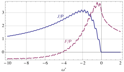
Figure 1: Dependence of $J$ (solid) and $F$ (dashed) on $\omega$, for $\omega_{c}^{*}=2$ and $d^{*}=20$.

To illustrate the significance of the dynamical poles, we choose $\mathcal{V}=\{0,\pm\Omega^{\prime}\}$. Note that $\Omega^{\prime}$ is the renormalised Rabi frequency, which is fixed once $H_{D}$ is chosen to eliminate dispersive shifts. The dispersive terms appearing in Eq. 6 are $f_{0}=a_{0}\,\sigma_{z}^{d}/2$, and $f_{\pm\Omega^{\prime}}=a_{\Omega^{\prime}}\,\sigma_{\pm}^{d}/2$ where

$$a_{0} =(-\alpha_{\omega_{0}-\Omega^{\prime}}^{2}F_{\omega_{0}-\Omega^{\prime}}+\alpha_{\omega_{0}+\Omega^{\prime}}^{2}F_{\omega_{0}+\Omega^{\prime}}+\alpha_{\Omega^{\prime}}^{2}F_{\Omega^{\prime}})/2,$$

$$a_{\Omega^{\prime}} =\alpha_{\omega_{0}}(\alpha_{\omega_{0}-\Omega^{\prime}}F_{\omega_{0}-\Omega^{\prime}}-\alpha_{\omega_{0}+\Omega^{\prime}}F_{\omega_{0}+\Omega^{\prime}})-\alpha_{0}\alpha_{\Omega^{\prime}}F_{\Omega^{\prime}},$$

and $F_{x}\equiv F(x)-F(-x)$. Setting $h_{\nu}=f_{\nu}$ to cancel dispersive terms yields the required relationship between the bare $\tilde{\eta},\tilde{\Omega}$ and the renormalised $\eta,\Omega$,

$$\left[\begin{array}[]{c}\tilde{\eta}\\ \tilde{\Omega}\end{array}\right]=-\left[\begin{array}[]{cc}\cos\varphi&-\sin\varphi\\ \sin\varphi&\cos\varphi\end{array}\right].\left[\begin{array}[]{c}a_{0}-\Omega^{\prime}\\ a_{\Omega^{\prime}}\end{array}\right].$$ (9)

We solve this nonlinear equation numerically for $\eta,\Omega$.

The renormalisation of the detuning arises from the phonon-induced Lamb shift Gardiner and Zoller (2000). This shift depends on the phonon modes with which the driven system is most strongly coupled, which depends itself on detuning Stace et al. (2005), resulting in a detuning-dependent Lamb shift. The renormalisation of the Rabi frequency is related to the polaron transformation Brandes and Kramer (1999); McCutcheon and Nazir (2013), in which pure-electronic modes are renormalised to polaronic modes with larger effective mass, reducing the transition dipole moments.

Differences between the bare and renormalised quantities ultimately depend on the electron-phonon coupling via $F$, which appears in $a_{0}$ and $a_{\Omega^{\prime}}$. Very close to resonance, $\tilde{\eta}\approx 0$, some intuition into the effect of the dispersive shifts can be gained by expanding the RHS of Eq. 9 in powers of $\Omega^{\prime}$ then solving to find

$$\eta_{\textrm{approx}} \approx{\tilde{\eta}}/({1+F^{\prime}(0)})+O[{\tilde{\eta}^{3}}/{\tilde{\Omega}^{2}}],$$ (10a)

$$\Omega_{\textrm{approx}} \approx{\tilde{\Omega}}/({1-F^{\prime}(0)})+O[{\tilde{\eta}^{2}}/{\tilde{\Omega}}].$$ (10b)

Thus, the renormalised detuning and Rabi frequency are scaled with respect to the bare values. Importantly, the scaling factors depend (non-perturbatively) on $F^{\prime}(0)$.

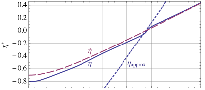
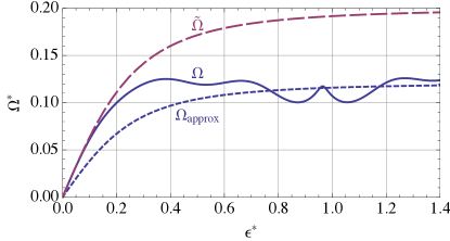
Figure 2: Top: Detuning versus bias. Bottom: Rabi frequency versus bias. Dashed curves: Bare detuning $\tilde{\eta}$ and Rabi frequency $\tilde{\Omega}$. Solid curves: Renormalised detuning $\eta$ and Rabi frequency $\Omega$ obtained by solving Eq. 9. Dotted curves: Near resonance approximations to renormalised quantities from Eq. 10; $\eta_{\textrm{approx}}$ captures the steeper slope of $\eta$ close to resonance. Parameters are $\Delta^{*}=0.3,\delta=\pi/2,\omega_{c}^{*}=2,d^{*}=20,\Omega_{0}^{*}=0.2,\mathsf{P}=0.2$. Resonance occurs at $\epsilon^{*}=(1-{\Delta^{*}}^{2})^{1/2}\approx 0.954$.

Focussing on the specific case of bulk piezo-electric phonon coupling, the spectral density is Stace et al. (2005)

$$J(\omega^{*})=\begin{cases}\pi\mathsf{P}|\omega^{*}|\frac{1-\mathrm{sinc}(d^{*}\omega^{*})}{1+(\omega^{*}/\omega_{c}^{*})^{2}}&\text{if }\omega^{*}<0\\ 0&\text{if }\omega^{*}\geq 0\end{cases}.$$ (11)

where $\omega^{*}\equiv\omega/\omega_{0},d^{*}\equiv d\,\omega_{0}/c_{s}$ and $\mathsf{P}$ are, respectively, nondimensionalised frequency, inter-dot separation, and coupling strength ($c_{s}$ is the speed of sound) . The high-energy cutoff, $\omega_{c}^{*}$, is determined by the spatial extent of the localised wavefunctions $|l\rangle,|r\rangle$. Fig. 1 shows $J$ and $F$ (which also has an analytic expression [SI]). The inter-dot separation results in double-slit-like interference as phonons interact with the localised states causing oscillations in $J$ and $F$, with a spectral period $\approx 2\pi/d^{*}$ Stace et al. (2005); Roulleau et al. (2011). This leads to a low frequency cut-off, $\sim 1/d^{*}$, in $J$. Between the low- and high-frequency cutoff, $J$ is Ohmic with a superimposed oscillatory modulation.

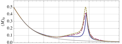
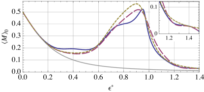
Figure 3: Top: Time-average steady-state population of the right dot, $\langle M\rangle_{0}=\langle|r\rangle\langle r|\rangle_{0}$, for relatively weak driving, $\Omega_{0}^{*}=0.07$. Bottom: $\langle M\rangle_{0}$ for stronger driving, $\Omega_{0}^{*}=0.2$. Inset: Zoom-in of red-detuned wing. Different curves correspond to different levels of approximation. Solid curve: $\mathcal{V}=\{0,\pm\Omega^{\prime}\}$ and renormalised $\eta,\Omega$. Dashed curve: $\mathcal{V}=\{0,\pm\Omega^{\prime}\}$ and bare $\tilde{\eta},\Omega_{\textrm{approx}}$. Dotted curve: $\mathcal{V}=\{0\}$ and bare $\tilde{\eta},\Omega_{\textrm{approx}}$. Light curve: No driving. Other parameters as in Fig. 2.

$F^{\prime}(0)$ determines the renormalisation strength. We can calculate $F^{\prime}(0)$ exactly [SI], but a good estimate is obtained by noting that $F^{\prime}(0)=-\pi^{-1}\int d\omega J(\omega)/\omega^{2}$. Combined with the facts that $J\approx\pi\mathsf{P}|\omega|$ for $\omega\in[-\omega_{c}^{*},-1/d^{*}]$ and it decays rapidly outside this interval we find that $F^{\prime}(0)\approx-\mathsf{P}\log(d^{*}\omega_{c}^{*})<0$. Thus the high- and low-frequency cut-offs appear as a ratio in the renormalisation strength. It follows from Eq. 10 that near resonance, the renormalised detuning is larger than the bare value, whilst the renormalised Rabi frequency is smaller.

Fig. 2 shows the effects of renormalisation on $\eta$ and $\Omega$. The renormalised quantities (solid curves) are modified most strongly close to resonance. Near resonance, the renormalised detuning is steeper than the bare detuning (dashed curve), consistent with the argument above. The renormalised Rabi frequency (bottom panel, solid curve) is lower than the bare value (dashed curve), and is well approximated by Eq. 10b near resonance.

The theoretical framework discussed here differs from Markovian models in two respects: it includes contributions arising from (a) the dynamical steady-state of the driven system, and (b) the bath-induced renormalisation of the system in which $H_{D}$ is chosen self-consistently to remove dispersive shifts and define the poles in $\mathcal{W}$. We elucidate these contributions by manually suppressing each effect, and comparing with the fully dynamical, renormalised result. We illustrate this by calculating the right dot population, $M=|r\rangle\langle r|=(1-\sigma_{z})/2$ Barrett and Stace (2006), which models an electrometer adjacent to the DQD Petta et al. (2004); Reilly et al. (2007).

Fig. 3 shows the time-averaged, steady-state population, $\langle M\rangle_{0}$, for relatively weak driving (top) and relatively strong driving (bottom). The solid curves show the dynamical, renormalised results; the dashed curve retains the dynamical poles but neglects renormalisation ; and the dotted curve neglects both, corresponding to the strong-driving Markov approximation Stace et al. (2005). The resonant peaks exhibit strong phonon-induced asymmetry, which becomes more pronounced at higher driving, to the extent of exhibiting population inversion on the blue-detuned side Dykman (1979); Stace et al. (2005). The enhancement of the blue-detuned wing is a consequence of photon absorption from the driving field accompanied by a Raman phonon emission, leading to a higher rate of excitation compared to the relaxation rate Stace et al. (2005). At weak driving, the resonant peak is unsaturated ($\langle M\rangle_{0}<0.5$), Fig. 3 (top), but this is only evident when dynamical poles are included (solid & dashed curves); suppressing dynamical poles necessarily yields a saturated peak on resonance, i.e. $\langle M\rangle_{0}=0.5$ at $\eta=0$, (dotted curves). Consistent with Fig. 2, the effects of parameter renormalisation are most significant near resonance, narrowing the central resonant peak. This occurs for two reasons: as $\epsilon$ moves away from resonance the renormalised detuning changes more rapidly with $\epsilon$ than does the bare detuning, and the renormalised Rabi frequency decreases below its resonant value.

Following Eq. 6 we noted that there are residual $F$-dependent terms in Eq. 6 that cannot be cancelled. This is manifest as subtle ‘shoulders’ appearing on the red-detuned side of the resonance ($\phi>\omega_{0}$), as shown in the inset to Fig. 3(bottom), resulting in non-Lorentzian decay of the red-detuned wings. In this regime, the microwave photons have insufficient energy to drive real transitions between the energy eigenstates, highlighting the fact that the shoulders are a consequence of dispersive, rather than dissipative, electron-phonon coupling.

Phenomena such as the transition from asymmetric unsaturated resonances at weak driving to population inversion at strong driving, and phonon-induced shoulders have been observed experimentally Colless et al. (2013). Our theory yields good qualitative agreement, and reasonable quantitative agreement with these experimental results. Intriguing connections exist between our approach and a non-Markovian extension to Redfield theory Ishizaki and Tanimura (2005, 2008).

In conclusion, we have derived a set of coupled equations for the residues of dynamical poles of the reduced density matrix of a system. These terms yield steady-state dynamics which are absent from Markovian treatments, as well as non-perturbative renormalisation of the bare system parameters. Neglecting either the dynamical poles or the effects of renormalisation yields qualitatively different results, particularly near resonance. The theory is consistent with recent experimental results which exhibit the same bath-induced phenomena discussed here. Our formalism permits arbitrarily many Floquet eigenfrequencies in the driven Hamiltonian, so extends straightforwardly to higher harmonics.

This research was supported by the Office of the Director of National Intelligence, Intelligence Advanced Research Projects Activity (IARPA), through the Army Research Office grant W911NF-12-1-0354 and by the Australian Research Council via the Centre of Excellence in Engineered Quantum Systems (EQuS), project number CE110001013. We thank S. Barrett, J. Colless, J. Coombes, X. Croote, G. Milburn, A. Nazir and A. Shabani for illuminating discussions.

References

- Braak (2011) D. Braak, Phys. Rev. Lett. 107, 100401 (2011).
- Gardiner and Zoller (2000) C. W. Gardiner and P. Zoller, Quantum Noise (Springer, 2000).
- Barrett and Stace (2006) S. D. Barrett and T. M. Stace, Phys. Rev. Lett. 96, 17405 (2006).
- Stace and Barrett (2004) T. M. Stace and S. D. Barrett, Phys. Rev. Lett. 92, 136802 (2004).
- Petta et al. (2004) J. R. Petta, A. C. Johnson, C. M. Marcus, M. P. Hanson, and A. C. Gossard, Phys. Rev. Lett. 93, 186802 (2004).
- Dykman (1979) M. I. Dykman, Sov. J. Low Temp. Phys. 5(2), 89 (1979).
- Brandes and Kramer (1999) T. Brandes and B. Kramer, Phys. Rev. Lett. 83, 3021 (1999).
- Stace et al. (2005) T. M. Stace, A. C. Doherty, and S. D. Barrett, Phys. Rev. Lett. 95, 106801 (2005).
- Roulleau et al. (2011) P. Roulleau, S. Baer, T. Choi, F. Molitor, J. Güttinger, T. Müller, S. Dröscher, K. Ensslin, and T. Ihn, Nat. Comm. 2, 239 (2011).
- Hanson et al. (2007) R. Hanson, L. P. Kouwenhoven, J. R. Petta, S. Tarucha, and L. Vandersypen, Rev. Mod. Phys. 79, 1217 (2007).
- Hayashi et al. (2003) T. Hayashi, T. Fujisawa, H. D. Cheong, Y. H. Jeong, and Y. Hirayama, Phys. Rev. Lett. 91, 226804 (2003).
- Oosterkamp et al. (1998) T. H. Oosterkamp, T. Fujisawa, W. G. van der Wiel, K. Ishibashi, R. V. Hijman, S. Tarucha, and L. P. Kouwenhoven, Nature 395 (1998).
- Fujisawa et al. (1998) T. Fujisawa, Oosterkamp, H. Tjerk, W. G. van der Wiel, B. W. Broer, R. Aguado, S. Tarucha, and L. Kouwenhoven, Science 282, 932 (1998).
- Granger et al. (2012) G. Granger, D. Taubert, C. E. Young, L. Gaudreau, A. Kam, S. A. Studenikin, P. Zawadzki, D. Harbusch, D. Schuh, W. Wegscheider, et al., Nat. Phys. 8, 522 (2012).
- Weber et al. (2010) C. Weber, A. Fuhrer, C. Fasth, G. Lindwall, L. Samuelson, and A. Wacker, Phys. Rev. Lett. 104, 036801 (2010).
- Ishizaki and Tanimura (2005) A. Ishizaki and Y. Tanimura, Journal of the Physical Society of Japan 74, 3131 (2005).
- McCutcheon and Nazir (2010) D. McCutcheon and A. Nazir, New J. Phys. 12, 113042 (2010).
- Maricq (1982) M. M. Maricq, Phys. Rev. B 25, 6622 (1982).
- Jeffreys and Jeffreys (1999) H. Jeffreys and B. Jeffreys, Methods of mathematical physics (Cambridge University Press, 1999).
- Stace et al. (2004) T. M. Stace, S. D. Barrett, H.-S. Goan, and G. J. Milburn, Phys. Rev. B 70, 205342 (2004).
- Mahan (1981) G. D. Mahan, Many-Particle Physics (Plenum Press, New York, 1981).
- Rahman et al. (2007) S. Rahman, T. M. Stace, H. Langtangen, M. Kataoka, and C. Barnes, Phys. Rev. B 75, 205303 (2007).
- McCutcheon and Nazir (2013) D. P. S. McCutcheon and A. Nazir, Phys. Rev. Lett. 110, 217401 (2013).
- Reilly et al. (2007) D. J. Reilly, C. M. Marcus, M. P. Hanson, and A. C. Gossard, Applied Physics Letters 91, 162101 (2007).
- Colless et al. (2013) J. I. Colless, X. G. Croot, T. M. Stace, A. C. Doherty, S. D. Barrett, H. Lu, A. C. Gossard, and D. J. Reilly, in review (2013), arXiv:1305.5982.
- Ishizaki and Tanimura (2008) A. Ishizaki and Y. Tanimura, Chem. Phys. 347, 185 (2008).