Recurrence Plots 25 years later – gaining confidence in dynamical transitions

Abstract

Recurrence plot based time series analysis is widely used to study changes and transitions in the dynamics of a system or temporal deviations from its overall dynamical regime. However, most studies do not discuss the significance of the detected variations in the recurrence quantification measures. In this letter we propose a novel method to add a confidence measure to the recurrence quantification analysis. We show how this approach can be used to study significant changes in dynamical systems due to a change in control parameters, chaos-order as well as chaos-chaos transitions. Finally we study and discuss climate transitions by analysing a marine proxy record for past sea surface temperature.
This paper is dedicated to the 25th anniversary of the introduction of recurrence plots.

Time series analysis statistical physics and nonlinear dynamics Sea surface temperature, paleoceanography Paleoclimatology

1 Introduction

In the November issue of EPL in 1987, Eckmann et al. proposed the recurrence plot as a tool to get easily insights into even high-dimensional dynamical systems [1, 2]. Over the last 25 years, their paper has “led to an active field, with many ramifications [these authors] certainly had not anticipated” [3]. Starting from the visual concept of recurrence plots (RPs), different statistical and quantification approaches have been added, like recurrence quantification (RQA), dynamical invariants from RPs, and recurrence networks [4, 5, 2, 6]. 25 years after Eckmann’s seminal paper, RPs and related methods are widely accepted tools for data analysis in various disciplines, as in physics [7] and chemistry [8], but also for real world systems as in life science [10, 9], engineering [11, 12], earth science [13], or finance and economy [14, 15, 16]. This interdisciplinary success is not only caused by the attractive appearance of RPs but also by the simplicity of the method [17]. Based on RPs, we can study the dynamics, transitions, or synchronisation of complex systems [1, 5, 2]. In particular, such transitions can be uncovered from a changing recurrence structure. The different aspects of recurrences can be inferred by measures of complexity, also known as recurrence quantification analysis (RQA). Although these measures are often applied on real data and interpreted as indicators of a change of the system’s dynamics, a statistical evaluation of the results was not yet satisfiably addressed. An early attempt has suggested to use a specific model class (e.g., auto-correlated noise) corresponding to the null-hypothesis and then testing the RQA results against such models [18]. For a general test of how significant the value of certain RQA measures (in particular determinism DET and laminarity LAM) is, a test distribution was derived using binomial distributions [19]. In order to compare time-dependent RQA measures of different observations, a bootstrap approach was introduced [20]. However, we still miss a method which can derive the important significance level of dynamical transitions within one dynamical system as indicated by RQA. Without providing some statement on the confidence of RQA results, any conclusions drawn from RQA might remain questionable [21].

In this letter we propose a method which calculates the confidence level for the most important, line-based RQA measures. We pick up the idea of bootstrapping [20] and develop a new algorithm allowing for gaining confidence in RQA based dynamical transition analysis. Using this approach we for the first time are able to provide a significance statement for detected transitions of not only qualitatively different systems dynamics based on RQA but using only a single observation. This will enable us to interpret the results of RQA in a more reliable way in the future research and, hence, will further increase the potentials and acceptance of RQA.

2 Recurrence Quantification Analysis

A RP tests for the pair-wise closeness of all possible pairs of states $(\vec{x}_{i},\vec{x}_{j})$ in an $m$-dimensional phase space, $R_{i,j}=\Theta\left(\varepsilon-d(\vec{x}_{i},\vec{x}_{j})\right)$, with $\Theta$ as the Heaviside function, $\varepsilon$ as a threshold for closeness [5, 22], and $i,j=1,\ldots,N$ where $N$ is the number of observed states. The closeness $d(\vec{x}_{i},\vec{x}_{j})$ can be measured in different ways, using, e.g., spatial distance, string metric or local rank order [5]. Most often, the spatial distance using maximum or Euclidean norm $d(\vec{x}_{i},\vec{x}_{j})=\|\vec{x}_{i}-\vec{x}_{j}\|$ is used. Then, the binary recurrence matrix $\mathbf{R}$ contains the value one for all close pairs $\|\vec{x}_{i}-\vec{x}_{j}\|<\varepsilon$. A phase space trajectory can be reconstructed from a time series by time delay embedding [23].

Similar evolving epochs of the phase space trajectory cause diagonal structures parallel to the main diagonal in the RP [5]. The length of such diagonal line structures depends on the dynamics of the system (periodic, chaotic, stochastic) and can be directly related with dynamically invariant properties, like $K_{2}$ entropy [5]. Therefore, the distribution $P(l)$ of line lengths $l$ is used by several RQA measures in order to characterise the system’s dynamics [5]. Here we focus on the measure determinism (DET), which is the fraction of recurrence points forming diagonal structures, $DET=\sum_{l=l_{\min}}^{N}l\,P(l)/\sum_{l=1}^{N}l\,P(l)$. A minimal length $l_{\min}$ defines a diagonal line [5].

Slowly changing states, as occuring during laminar phases (intermittency), cause vertical structures in the RP. Therefore, the distribution $P(v)$ of line lengths $v$ is used to quantify the laminar phases occuring in a system. Similar to DET, the measure laminarity (LAM) is defined as the fraction of the recurrence points forming vertical structures, $LAM=\sum_{v=v_{\min}}^{N}v\,P(v)/\sum_{v=1}^{N}v\,P(v)$ [9].

The later discussed approach will not only be applicable to these two measures DET and LAM, but to all line based RQA measures, including recurrence time based measures [24].

In order to study time dependent behaviour of a system or data series, we compute these RQA measures using a moving window, applied on the time series. The window has size $w$ and is moved with a step size $s$ over the data in such a way that succeeding windows overlap with $w-s$. This technique was successfully applied to detect chaos-period transitions [25], but also more subtle ones such as chaos-chaos transitions [9], or different kinds of transitions between strange non-chaotic behaviour and period or chaos [26]. It is applicable to real world data, as demonstrated for the study of, e.g., cardiac variability [27], brain activity [28], changes in finance markets [29] or thermodynamic transitions in corrosion processes [12]. However, all these applications miss a clear significance statement.

With respect to our goal of a transition detection in the dynamical system, we formulate the following null-hypothesis $\mathcal{H}_{0}$: The dynamics of a system $X$ does not change over time, thus, the recurrence structure does not change and the RQA measure $M$ of such a system will therefore be distributed around an unknown, but non-zero mean $\mu(M)$ with unknown variance $\sigma(M)$.

For completely random systems the expected distribution of some RQA measures can be modeled [19]. However, for complex real systems it cannot be assumed that the underlying recurrence structure is completely random but rather features a certain recurrence structure at all times. A dynamical transition in the system changes the recurrence structure and, hence, the RQA measures. If the impact of the transition is large enough, it will push the RQA measure $M$ out of its normal range. The deviation from this normal range can be considered as significant if the observed value of $M(t)$ at time point $t$ is outside of a predefined interquantile range such as $[\alpha/2,\ 1-\alpha/2]$.

3 Variance estimation by bootstrapping

In order to test for significant deviations from the unknown mean of the data, we first have to estimate the variance of the RQA measures in question. To do so, we introduce a bootstrap approach in the calculation of the RQA measures [30]. Bootstrapping is a conceptually simple yet powerful statistical tool to estimate the variance of statistical parameters, such as the mean, even if the underlying distribution is unknown. Since we cannot assume that the distributions of line lengths $P(l)$ and $P(w)$ follow a known probability distribution, we use this advantage of the bootstrap approach to estimate the confidence bounds of the RQA measures $M$ which rely on these distributions. We will use bootstrap resampling to create a test distribution of the RQA measures from which we can then estimate the overall mean and variance of those measures and, finally, to formulate the important significance statement.

The time dependent RQA analysis is based on moving windows, shifted over the time series, and calculating the RP within these windows. For each of the $N_{\rm w}$ time steps of the moving window $t$ ($t=w/2,3w/2,5w/2,\dots,N-w/2$), i.e., for different time points, we get the local RPs with $n(t)$ diagonal lines and then calculate the corresponding local histograms of diagonal lines $P_{t}(l)$. The time dependent RQA measures $M(t)$ (e.g., $M(t)=DET(t)$ are calculated from $P_{t}(l)$.

In order to estimate a general distribution of the RQA measures following our null-hypothesis $\mathcal{H}_{0}$, we suggest the following procedure. All local histograms $P_{t}(l)$ are merged together in order to get an overall histogram and thus a statistical average of the recurrence structure of the system, i.e., we bootstrap from the unification

$$\hat{P}(l)=\sum_{t}P_{t}(l)$$ (1)

of the local histograms. We draw $\bar{n}$ recurrence structures (i.e. diagonal lines) from $\hat{P}(l)$. The number $\bar{n}$ of drawings is the mean number of recurrence structures $n(t)$ contained in the local distributions $P_{t}(l)$,

$$\bar{n}=\frac{1}{N_{\rm w}}\sum_{t=w/2}^{N-w/2}n(t)=\frac{1}{N_{\rm w}}\sum_{t=w/2}^{N-w/2}\sum_{l=1}^{N}P_{t}(l).$$ (2)

From the resulting empirical distribution $P(l)^{*}$, we compute the corresponding RQA measure, say in our case DET. By repeating this procedure $B$ times (e.g. $B=1,000$), we get the test distribution for DET, say $F(DET)$. By calculation of the $\alpha$-quantiles of the distribution $F(DET)$, we derive the confidence intervals of DET which can be used to statistically infer the significance of the changes of $DET(t)$, and thus the observed transitions.

4 Illustration of the method

We illustrate the proposed statistical test on two model systems: (1) a linear autocorrelated process and (2) a nonlinear process, both for changing parameters.

(1) Our first example is an autocorrelated stochastic signal with changing properties, i.e., an autoregressive process of order 2

$$x_{i}=a_{1}x(i-1)+a_{2}x(i-2)+b\xi(i)$$ (3)

with $a_{1}=1.80$, $a_{2}=-0.972$ and $b=0.64$. After time step 1,300, the AR coefficients slightly change to $a_{1}=1.85$, $a_{2}=-0.917$ and $b=0.76$ for 500 time steps. Afterwards these coefficients are changed back to the initial values. With this procedure the signal contains a short epoch of slightly changed dynamics (Fig. 1A).

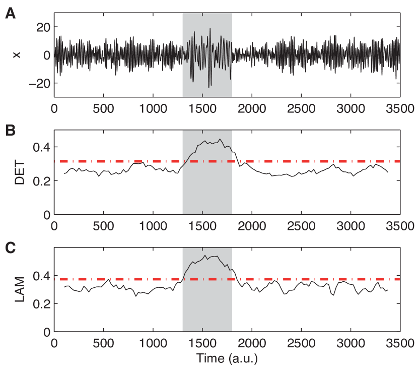
Figure 1: (Colour online) (A) Autocorrelated process with slight transitions of the parameters between time 1,300 and 1,800 (shaded region). Corresponding RQA measures (B) determinism DET and (C) laminarity LAM, indicating the epoch of changed dynamics in the autocorrelated process between 1,300 and 1,800 (shaded area) by an increasing of their values. This increase exceeds the 99% confidence interval (dashed line) as derived by the proposed bootstrapping approach.

Next we compute the RQA measures DET and LAM from this data series (no embedding) using windows of size $w=200$ and with a step size of $s=25$. The threshold $\varepsilon$ is chosen for each window separately to preserve a constant recurrence rate of 7.5% [22]. The bootstrap resampling is then applied using 1,000 resamplings. As we expect in the window of increased auto-correlation a larger number of diagonal and vertical lines, we will only consider the upper confidence level.

The DET measure reveals a high number of diagonal lines in the RP. Before time 1,300 and after time 1,800, DET values vary between 0.25 and 0.3. This coincides with the moderate auto-correlation of the process. Between the time 1,300 and 1,800, DET shows an increase and exceeds the confidence interval of 0.31, corresponding to a 99% confidence level. Similar, LAM varies before and after the inset of changed dynamics at a lower level ($LAM\approx 0.3$) and increases within the period between time 1,300 and 1,800 up to $LAM\approx 0.55$ due to its increased persistence. This increase of DET and LAM confirms the further increase of the auto-correlation of the considered process within this epoch.

(2) To test whether the proposed method is also capable of providing a quanatitative statement of more subtle changes in dynamics, like chaos-order and chaos-chaos transitions, we use a modified logistic map with mutual transitions [25]

$$x_{i+1}=a(i)x(i)(1-x(i))$$ (4)

with the control parameter $a$ in the range $[3.9200\ 3.9335]$ with increments of $\Delta a=2.5\ 10^{-7}$. Using this intervall we find for $a=[3.92221\ 3.92227]$ a period-7 window, for $a=[3.93047\ 3.93050]$ a period-8 window and at a broad range around $a=3.928\dots$ intermittency (Fig. 2). Again, for these kind of dynamical transitions we can expect increased values of DET and LAM, hence, we only need to consider the upper confidence level.

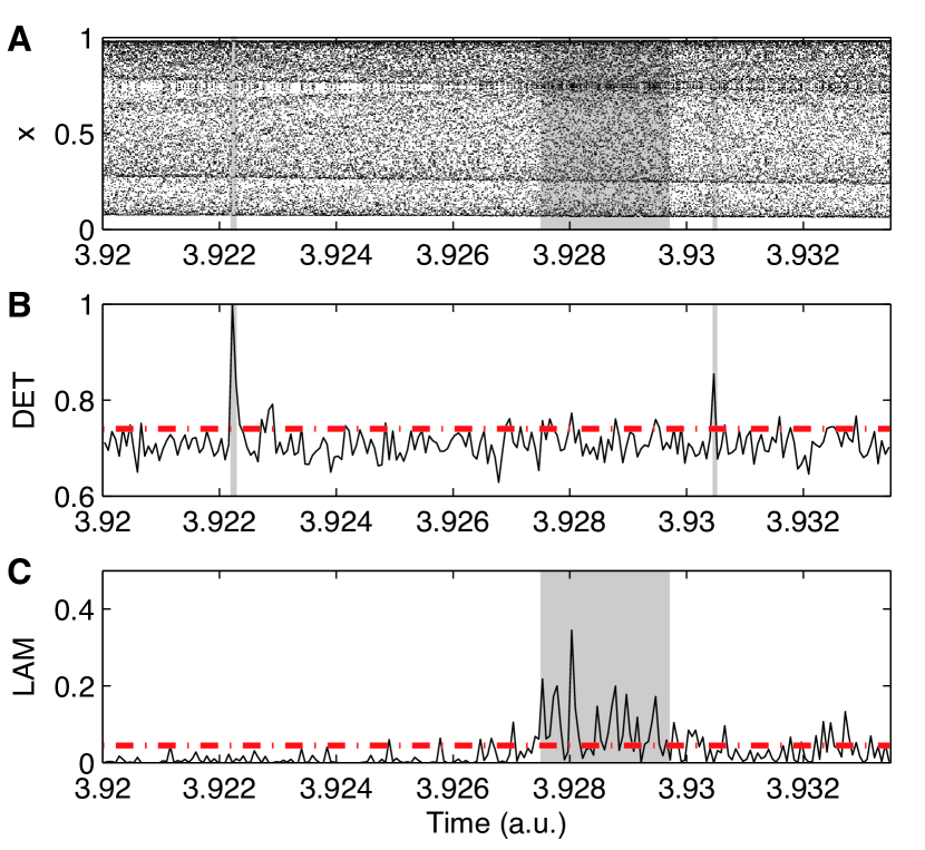
Figure 2: (A) Logistic map with chaos-period and chaos-chaos transitions for control parameter $a=[3.9200\ 3.9335]$ and corresponding RQA measures (B) DET and (C) LAM. For $a=[3.92221\ 3.92227]$ we have a period-7 window, for $a=[3.93047\ 3.93050]$ a period-8 window and at a broad range around $a=3.928$ intermittency (marked with shaded area). (B) and (C) 99% significance levels are shown as dash-dotted lines.

Next we compute the RQA measures DET and LAM from this data series (no embedding) using windows of size $w=250$ and with a step size of $s=250$. The threshold $\varepsilon$ is chosen for each window separately in order to preserve a constant recurrence rate of 5%. As a line structure we consider each line with a length of at least two points, i.e. $l_{\min}=v_{\min}=2$.

The measure DET shows for the periodic windows at $a=[3.92221\ 3.92227]$ and $a=[3.93047\ 3.93050]$ maxima [9]. The periodic behaviour of the system causes only long diagonal lines, resulting in high values of DET. In contrast, LAM shows high values only for the region of intermittency around $a=3.928\dots$. In this region, the system has slowly changing, laminar states [9]. For the proposed bootstrapping approach, we use 1,000 resamplings in order to construct the test statistics. As the 99%-quantile we find for DET $q_{0.99}=0.74$ and for LAM $q_{0.99}=0.04$. These values provide the 99% confidence level for DET and LAM. Thus, the two maxima of DET in the periodic windows are significant on a 99% level ( p $<$ 0.01). For LAM we find several significant high values of 99% significance in the region of intermittency around $a=3.928$. This is due to the longer range of intermittent behaviour in this region of the control parameter $a$.

5 Application to real world data

The climate system is a highly complex one which has undergone various transitions in the past. The investigation of relationships between sea surface temperature (SST) and specific climate responses, like the Asian monsoon system or the thermohaline circulation in the Atlantic, represents an important scientific challenge for understanding the global climate system, its mechanisms, and its related variability. In palaeoclimatology, different archives are used to reconstruct and study climate conditions of the past, as lake [18] and marine sediments [31] or speleothemes [32]. Alkenone remnants in the organic fraction of marine sediments, produced by phytoplankton, can be used to reconstruct SST of the past, allowing to study the temperature variability of the oceans [33]. Here we will use a marine record from the Ocean Drilling Programme (ODP) derived from a drilling in the Arabian see, ODP site 722. This record provides alkenone based reconstructed SST in the realm of the Asian monsoon system for the past 3.3 Ma (Fig. 3A) [31]. During this epoch, a dramatic climate change happened by two steps of global cooling [31]. The first step between 3.0 and 2.5 Ma coincides with the high-latitude Northern Hemisphere glaciation. The second step of cooling occurred between 2.0 and 1.5 Ma and is related with a continuous cooling of the subtropical oceans but a stationary high-latitude climate. Some mechanisms of these global-scale climate changes are known and coincide with a transition to an obliquity-driven climate variability with a 41 ka period after 2.8–2.7 Ma [31], a shift from that climate variability (with high-latitude glaciation) to glacial-interglacial cycles with a 100 ka period after a transition period between 1.25 and 0.7 Ma [34], and the development of the Walker circulation at 1.9–1.5 Ma [35]. The RQA and the proposed significance test are promising tools to analyze the alkenone SST record of the ODP site 722.

The original time series of ODP 722 is not equally sampled. Therefore, we interpolate it to a time series with sampling period of 2 ka. For performing the RQA we use a time delay embedding with dimension $m=3$ and delay $\tau=2$. The threshold is chosen to preserve a constant recurrence rate of 7.5%. The bootstrapping is performed using 1,000 resamplings. In this real world example, we use a reduced confidence level of 95%. As we do not know which kinds of dynamical transition are there, we will consider both the upper and the lower confidence level.

The RQA measures DET and LAM reveal various significantly high and low values as summarised in Fig. 3 and Tab. 1.

[width=]fig_rqa_odp722

Figure 3: (A) Alkone SST record of ODP site 722, and corresponding (B) DET and (C) LAM measures (95% confidence bounds are shown with blue dash-dotted lines). The transition to (1) the Northern Hemisphere glaciation, the (2) intensification of the Walker circulation, and (3) the transition phase from glaciation to glacial-interglacial cycles are marked by shaded areas.

Around 3.0 Ma ago, a long-lasting period of warm climate with a permanent El Niño came to an end. This general change from a warm climate towards a more variable and cooler one is clearly indicated by a change from low to high DET and LAM values.

The first cooling phase between 3.0 and 2.5 Ma is well indicated by high values of the measure DET which can be considered to reflect an increase in regularity and auto-correlation of the system. The rapid onset of the Northern Hemisphere glaciation between 2.8 and 2.7 Ma is marked by an increase of LAM, corresponding to an intermittent behaviour. The fact that DET and, thus, the auto-correlation increased before the intermittent behaviour can be understood as a critical slowing down of the dynamics as it is typical for tipping points [36]. The increase of DET might, therefore, be an indication that the climate system reached a tipping point at 3.0–2.9 Ma, leading to the regime change of Northern Hemisphere glaciation.

Between 2.4 and 2.3 Ma, DET and LAM decreased, revealing a short period of more irregular and stochastic variability. This might be an indication for a transition between two different regimes. This transition was not yet found in palaeoclimate literature, but is confirmed by another study also using a nonlinear measure for transition detection [37].

The period of the development of the Walker circulation between 1.9 and 1.5 Ma is marked by an increase in both, DET and LAM.

The transition period from the glaciation regime with dominant 41 ka cycle to the glacial-interglacial regime with 100 ka cycle is marked by a significant decrease of the measures DET and LAM. This corresponds to a phase of less regularity or more stochastic variability of the SST.

Further high values in DET and LAM occur at around 2.0 Ma and between 0.75 and 0.5 Ma. At 2.0 Ma, a reorganization of subtropical and tropical ocean circulation begun which was triggered by high-latitude cooling and its impact on deepwater formation. Between 0.75 and 0.5 Ma, the sensitivity of the high-latitude climate response to solar forcing reached its maximum [35]. This is consistent with recent findings of a coherence between solar forcing and climate variability in this region during this period [37].

The transitions found correspond to dynamical transitions caused by different changes in climate. The recurrence based analysis can not only detect these transitions but also provide additional information about the climate transitions, whose onsets are, at least partly, known [38, 37].

Table 1: Major regime changes in alkenone SST record from ODP site 722 as indicated by significant high values of determinism (DET$+$) and laminarity (LAM$+$) as well as significant low values (DET$-$ and LAM$-$).

Period	DET$+$	DET$-$	LAM$+$	LAM$-$
Northern Hemisphere glaciation	2.9–2.5		2.75–2.65
Interregime transition		2.4–2.3		2.4–2.3
(Sub-)Tropical reorganisation	2.0		2.05–1.95
Development Walker circulation	1.7–1.4		1.7–1.5
Transition 41 ka to 100 ka		1.25–0.8		1.2–0.8
Maximal climate sensitivity	0.65-0.55		0.75–0.5

6 Conclusion

We have introduced a bootstrap based approach for providing confidence levels for line-based recurrence quantification measures, which are related to dynamical properties (like Lyapunov exponent or $K_{2}$ entropy). Using this technique, we are able to investigate changing dynamics by RQA and can, for the first time, provide confidence levels for the variation of the RQA measures and, thus, the changed dynamics. We have shown the potential of the approach by studying dynamical changes in an auto-correlated process and for chaos-order and chaos-chaos transitions. These examples have also demonstrated the importance of considering confidence intervals, as fluctuations in the RQA measures can be misinterpreted if the overall variance of these measures is not taken into consideration.

The application of our approach on sea surface temperature variability of the past has demonstrated that recurrence based analysis provides new insights in known palaeo-climate changes. Recurrence properties can be help for a better understanding of the mechanisms of the transitions between different climate regimes.

25 years after the introduction of recurrence plots by Eckmann et al. [1], the development of this technique still continues. With our paper we would like to honor the seminal work by these authors, but would also like to emphasize that the calculation of confidence levels for the RQA measures is an important requirement for the method to get widely accepted. It is highly desirable that future research using RQA comes along with corresponding confidence levels.

- [1] \NameEckmann J.-P., Oliffson Kamphorst S. Ruelle D. \REVIEWEurophysics Letters51987973.
- [2] \NameMarwan N. \REVIEWEuropean Physical Journal – Special Topics16420083.
- [3] \NameMarwan N., Facchini A., Thiel M., Zbilut J. P. Kantz H. \REVIEWEuropean Physical Journal – Special Topics16420081.
- [4] \NameWebber Jr. C. L. Zbilut J. P. \REVIEWJournal of Applied Physiology761994965. \NameZbilut J. P. Webber Jr. C. L. \REVIEWInternational Journal of Bifurcation and Chaos1720073477.
- [5] \NameMarwan N., Romano M. C., Thiel M. Kurths J. \REVIEWPhysics Reports4382007237.
- [6] \NameDonner R. V., Zou Y., Donges J. F., Marwan N. Kurths J. \REVIEWNew Journal of Physics122010033025.
- [7] \NameVretenar D., Paar N., Ring P. Lalazissis G. A. \REVIEWPhysical Review E601999308. \NameJamitzky F., Stark M., Bunk W., Heckl W. M. Stark R. W. \REVIEWNanotechnology172006S213.
- [8] \NameRustici M., Caravati C., Petretto E., Branca M. Marchettini N. \REVIEWJournal of Physical Chemistry A10319996564. \NameGarcía-Ochoa E., González-Sánchez J., na N. A. Euan J. \REVIEWJournal of Applied Electrochemistry392009637.
- [9] \NameMarwan N., Wessel N., Meyerfeldt U., Schirdewan A. Kurths J. \REVIEWPhysical Review E662002026702.
- [10] \NameZbilut J. P., Giuliani A., Colosimo A., Mitchell J. C., Colafranceschi M., Marwan N., Uversky V. N. Webber Jr. C. L. \REVIEWJournal of Proteome Research320041243. \NameStam C. J. \REVIEWClinical Neurophysiology11620052266. \NameSchinkel S., Marwan N. Kurths J. \REVIEWCognitive Neurodynamics12007317.
- [11] \NameNichols J. M., Trickey S. T. Seaver M. \REVIEWMechanical Systems and Signal Processing202006421. \NameSen A. K., Longwic R., Litak G. Górski K. \REVIEWMechanical Systems and Signal Processing222008362.
- [12] \NameMontalbán L. S., Henttu P. Piché R. \REVIEWInternational Journal of Bifurcation and Chaos1720073725.
- [13] \NameMarwan N., Donges J. F., Zou Y., Donner R. V. Kurths J. \REVIEWPhysics Letters A37320094246. \NameMarch T. K., Chapman S. C. Dendy R. O. \REVIEWGeophysical Research Letters3220051. \NameZolotova N. V. Ponyavin D. I. \REVIEWSolar Physics2432007193.
- [14] \NameBelaire-Franch J., Contreras D. Tordera-Lledó L. \REVIEWPhysica D1712002249.
- [15] \NameCrowley P. M. Schultz A. \REVIEWInternational Journal of Bifurcation and Chaos2120111215.
- [16] \NameGoswami B., Ambika G., Marwan N. Kurths J. \REVIEWPhysica A39120124364.
- [17] \NameWebber Jr. C. L., Marwan N., Facchini A. Giuliani A. \REVIEWPhysics Letters A37320093753.
- [18] \NameMarwan N., Trauth M. H., Vuille M. Kurths J. \REVIEWClimate Dynamics212003317.
- [19] \NameHirata Y. Aihara K. \REVIEWInternational Journal of Bifurcation and Chaos2120111077.
- [20] \NameSchinkel S., Marwan N., Dimigen O. Kurths J. \REVIEWPhysics Letters A37320092245.
- [21] \NameMarwan N. \REVIEWInternational Journal of Bifurcation and Chaos2120111003.
- [22] \NameSchinkel S., Dimigen O. Marwan N. \REVIEWEuropean Physical Journal – Special Topics164200845.
- [23] \NamePackard N. H., Crutchfield J. P., Farmer J. D. Shaw R. S. \REVIEWPhysical Review Letters451980712.
- [24] \NameNgamga E. J., Senthilkumar D. V., Prasad A., Parmananda P., Marwan N. Kurths J. \REVIEWPhysical Review E852012026217.
- [25] \NameTrulla L. L., Giuliani A., Zbilut J. P. Webber Jr. C. L. \REVIEWPhysics Letters A2231996255.
- [26] \NameNgamga E. J., Nandi A., Ramaswamy R., Romano M. C., Thiel M. Kurths J. \REVIEWPhysical Review E752007036222.
- [27] \NameZbilut J. P., Thomasson N. Webber Jr. C. L. \REVIEWMedical Engineering & Physics24200253.
- [28] \NameSchinkel S., Marwan N. Kurths J. \REVIEWJournal of Physiology-Paris1032009315.
- [29] \NameStrozzi F., Zaldívar J.-M. Zbilut J. P. \REVIEWPhysica A3122002520.
- [30] \NameEfron B. Tibshirani R. J. \BookAn Introduction to the Bootstrap (Chapman & Hall/CRC, Boca Raton, London, New York, Washington DC) 1998.
- [31] \NameHerbert T. D., Peterson L. C., Lawrence K. T. Liu Z. \REVIEWScience (New York, N.Y.)32820101530.
- [32] \NameKennett D. J., Breitenbach S. F. M., Aquino V. V., Asmerom Y., Awe J., Baldini J. U. L., Bartlein P., Culleton B. J., Ebert C., Jazwa C., Macri M. J., Marwan N., Polyak V., Prufer K. M., Ridley H. E., Sodemann H., Winterhalder B. Haug G. H. \REVIEWScience3382012788.
- [33] \NameHerbert T. D. \REVIEWGeochemistry Geophysics Geosystems220011005.
- [34] \NameMudelsee M. Schulz M. \REVIEWEarth and Planetary Science Letters1511997117.
- [35] \NameRavelo A. C., Andreasen D. H., Lyle M., Lyle A. O. Wara M. W. \REVIEWNature4292004263.
- [36] \NameDakos V., Scheffer M., van Nes E. H., Brovkin V., Petoukhov V. Held H. \REVIEWProceedings of the National Academy of Sciences of the United States of America105200814308. \NameScheffer M., Bascompte J., Brock W. A., Brovkin V., Carpenter S. R., Dakos V., Held H., van Nes E. H., Rietkerk M. Sugihara G. \REVIEWNature461200953.
- [37] \NameMalik N., Zou Y., Marwan N. Kurths J. \REVIEWEurophysics Letters (EPL)97201240009.
- [38] \NameDonges J. F., Donner R. V., Trauth M. H., Marwan N., Schellnhuber H. J. Kurths J. \REVIEWProceedings of the National Academy of Sciences108201120422.