Predictability of Event Occurrences
in Timed Systems

Abstract

We address the problem of predicting events’ occurrences in partially observable timed systems modelled by timed automata. Our contribution is many-fold: 1) we give a definition of bounded predictability, namely $k$-predictability, that takes into account the minimum delay between the prediction and the actual event’s occurrence; 2) we show that $0$-predictability is equivalent to the original notion of predictability of S. Genc and S. Lafortune; 3) we provide a necessary and sufficient condition for $k$-predictability (which is very similar to $k$-diagnosability) and give a simple algorithm to check $k$-predictability; 4) we address the problem of predictability of events’ occurrences in timed automata and show that the problem is PSPACE-complete.

1 Introduction

Monitoring and fault diagnosis aim at detecting defects that can occur at run-time. The monitored system is partially observable but a formal model of the system is available which makes it possible to build (offline) a monitor or a diagnoser. Monitoring and fault diagnosis for discrete event systems (DES) have been have been extensively investigated in the last two decades [1, 2, 3]. Fault diagnosis consists in detecting a fault as soon as possible after it occurred. It enables a system operator to stop the system in case something went wrong, or reconfigure the system to drive it to a safe state. Predictability is a strong version of diagnosability: instead of detecting a fault after it occurred, the aim is to predict the fault before its occurrence. This gives some time to the operator to choose the best way to stop the system or to reconfigure it.

In this paper, we address the problem of predicting event occurrences in partially observable timed systems modelled by timed automata.

The Predictability Problem. A timed automaton [4] (TA) generates a timed language which is a set of timed words which are sequences of pairs (event, time-stamp). Only a subset of the events generated by the system is observable. The objective is to predict occurrences of a particular event (observable or not) based on the sequences of observable events. Automaton $G$, Fig. 1, is a timed version of the example of automaton $G_{1}$ of [5]. The set of observable events is $\{a,b,c\}$. We would like to predict event $f$ without observing event $d$.

Figure 1: Example $G$ from [5].

First consider the untimed version of $G$ by ignoring the constraints on clock $x$. The untimed automaton can generate two types of events’ sequences: $d.a.b^{*}$ and $a.c.f.\{a,b,c\}^{*}$. Because $d$ is unobservable, after observing $a$ we do not know whether the system is in location $l_{4}$ or $l_{1}$ and cannot predict $f$ as, according to our knowledge, it is not bound to occur in all possible futures from locations $l_{4}$ or $l_{1}$. However, after the next observable event, $b$ or $c$, we can make a decision: if we observe $a.c$, $G$ must be in $l_{2}$ and thus $f$ is going to happen next. After observing $a.c$ we can predict event $f$. Note that there is no quantitative duration between occurrences of events in discrete event systems and thus we can predict $f$ at a logical time which is before $f$ occurs. The time that separates the prediction of $f$ from the actual occurrence of $f$ is measured in the number of discrete steps $G$ can make. In this sense $G$ is $0$-predictable as when we predict $f$, it is the next event to occur. The untimed version of $G$ is an abstraction of a real system, and in the real system, it could be that $f$ is going to occur 5 seconds after we observe $c$.

Timed automata enable us to capture quantitative aspects of real-time systems. We can use clocks (like $x$) to specify constraints between the occurrences of events. Moreover invariants (like $[x\leq 1]$) ensure that $G$ changes location when the upper bound of the invariant is reached. In the timed automaton $G$, the (infinite) sequences with no $f$ are of the form $(d,\delta_{d})(a,\delta_{a})(b,\delta_{b})\cdots$ with $\delta_{d}<1,\delta_{a}\leq 1$ and $\delta_{b}<2$. The sequences with event $f$ are of the form $(a,1)(c,3)(f,\delta_{f})$ with $5\leq\delta_{f}\leq 6$. Thus if we do not observe a “b” within the first two time units, we know that the system is in location $l_{1}$. This implies that $f$ is going to occur, and we know this at time $2$. But $f$ will not occur before $1+2$ time units, the time for $c$ to occur (from time $2$) and the minimum time for $f$ to occur after $c$. $G$ is thus $3$-predictable. In the sequel we formally define the previous notions and give efficient algorithms to solve the predictability problem.

Related Work. Predictability for discrete event systems was first proposed by S. Genc and S. Lafortune in [6]. Later in [5] they gave two algorithms to decide the predictability problem, one of them is a polynomial decision procedure. T. Jéron, H. Marchand, S. Genc and S. Lafortune [7] extended the previous results to occurrences of patterns (of events) rather than a single event. L. Brandán Briones and A. Madalinski in [8] studied bounded predictability without relating it to the notion defined by S. Genc and S. Lafortune.

Predictability is closely related to fault diagnosis [1, 2, 3]. The objective of fault diagnosis is to detect the occurrence of a special event, a fault, which is unobservable, as soon as possible after it occurs. Fault diagnosis for timed automata has first been studied by S. Tripakis in [9] and he proved that the diagnosis problem is PSPACE-complete. P. Bouyer, F. Chevalier and D. D’Souza [10] later studied the problem of computing a diagnoser with fixed resources (a deterministic TA) and proved that this problem is 2EXPTIME-complete. To the best of our knowledge the predictability problem for TA has not been investigated yet.

Our Contribution. We give a new characterization of bounded predictability and show it is equivalent to the definition of S. Genc and S. Lafortune. This new characterization is simple and dual to the one for the diagnosis problem; we can derive easily algorithms to decide predictability, bounded predictability, and to compute the largest anticipation delay to predict a fault. We also study the bounded predictability problem for TA and prove it is PSPACE-complete. We investigate implementability issues, i.e., how to build a predictor, and solve the sampling predictability problem which ensures an implementable predictor exists. We show how to compute bounded predictability with Uppaal [11].

Organization of the Paper. The paper is organized as follows: the next section recalls some definitions: timed words, timed automata. Section 3 states the predictability problems for TA and Finite Automata (FA) and presents a necessary and sufficient condition for bounded predictability. Section 4 compares our definition of predictability with the original one (by S. Genc and S. Lafortune) and provides an algorithm (for finite automata) to solve the bounded predictability problem and compute the largest bound. Section 5 studies the bounded predictability problem for TA and implementation issues related to the construction of a predictor. An example is also solved with Uppaal. Omitted proofs are given in Appendix.

2 Preliminaries

$\mathbb{B}=\{\mbox{{true}},\mbox{{false}}\}$ is the set of boolean values, $\mathbb{N}$ the set of natural numbers, $\mathbb{Z}$ the set of integers and $\mathbb{Q}$ the set of rational numbers. $\mathbb{R}$ is the set of real numbers and $\mathbb{R}_{\geq 0}$ is the set of non-negative reals.

2.1 Clock Constraints

Let $X$ be a finite set of variables called clocks. A clock valuation is a mapping $v:X\rightarrow\mathbb{R}_{\geq 0}$. We let $\mathbb{R}_{\geq 0}^{X}$ be the set of clock valuations over $X$. We let $\mathbf{0}_{X}$ be the zero valuation where all the clocks in $X$ are set to $0$ (we use $\mathbf{0}$ when $X$ is clear from the context). Given $\delta\in\mathbb{R}$, $v+\delta$ denotes the valuation defined by $(v+\delta)(x)=v(x)+\delta$. We let ${\cal C}(X)$ be the set of convex constraints on $X$ which is the set of conjunctions of constraints of the form $x\bowtie c$ with $c\in\mathbb{N}$ and $\bowtie\in\{\leq,<,=,>,\geq\}$. Given a constraint $g\in{\cal C}(X)$ and a valuation $v$, we write $v\models g$ if $g$ is satisfied by $v$. Given $R\subseteq X$ and a valuation $v$, $v[R]$ is the valuation defined by $v[R](x)=v(x)$ if $x\not\in R$ and $v[R](x)=0$ otherwise.

2.2 Timed Words

A finite (resp. infinite) timed word over $\Sigma$ is a word in $\mathbb{R}_{\geq 0}.(\Sigma.\mathbb{R}_{\geq 0})^{*}$ (resp. $(\mathbb{R}_{\geq 0}.\Sigma)^{\omega}$). We write timed words as $0.4\ a\ 1.0\ b\ 2.7\ c\cdots$ where the real values are the durations elapsed between two events: thus $c$ occurs at global time $4.1$. We let ${\textit{Dur}}(w)$ be the duration of a timed word $w$ which is defined to be the sum of the durations (in $\mathbb{R}_{\geq 0}$) which appear in $w$; if this sum is infinite, the duration is $\infty$. Note that the duration of an infinite word can be finite, and such words which still contain an infinite number of events, are called Zeno words. An infinite timed word $w$ is time-divergent if ${\textit{Dur}}(w)=\infty$. We let $\textit{Unt}(w)$ be the untimed version of $w$ obtained by erasing all the durations in $w$, e.g., $\textit{Unt}(0.4\ a\ 1.0\ b\ 2.7\ c\ 0)=abc$. Given $w$ a timed word and $a\in\Sigma$, $|w|_{a}$ is the number of occurrences of $a$ in $w$ ($\infty$ if $a$ occurs infinitely often in $w$.)

$\textit{TW\/}^{*}(\Sigma)$ is the set of finite timed words over $\Sigma$, $\textit{TW\/}^{\omega}(\Sigma)$, the set of infinite timed words and $\textit{TW\/}^{\infty}(\Sigma)=\textit{TW\/}^{*}(\Sigma)\cup\textit{TW\/}^{\omega}(\Sigma)$. We use $\Sigma^{*}$ and $\Sigma^{\omega}$ for the corresponding sets of untimed words. A timed language is any subset of $\textit{TW\/}^{\infty}(\Sigma)$. For $L\subseteq\textit{TW\/}^{\infty}(\Sigma)$, we let $\textit{Unt}(L)=\{\textit{Unt}(w)\ |\ w\in L\}$.

For $w\in\textit{TW\/}^{*}(\Sigma)$ and $w^{\prime}\in\textit{TW\/}^{\infty}(\Sigma)$, $w.w^{\prime}$ is the concatenation of $w$ and $w^{\prime}$. A finite timed word $w$ is a prefix of $w^{\prime}\in\textit{TW\/}^{\infty}(\Sigma)$ if $w^{\prime}=w.w^{\prime\prime}$ for some $w^{\prime\prime}\in\textit{TW\/}^{\infty}(\Sigma)$. In the sequel we also the prefix operator and $\overline{L}$ is the set of finite words that are prefixes of words in $L$.

Let $\Sigma_{1}\subseteq\Sigma$. $\boldsymbol{\pi}_{/\Sigma_{1}}$ is the projection of timed words of $\textit{TW\/}^{\infty}(\Sigma)$ over timed words of $\textit{TW\/}^{\infty}(\Sigma_{1})$. When projecting a timed word $w$ on a sub-alphabet $\Sigma_{1}\subseteq\Sigma$, the durations elapsed between two events are set accordingly: $\boldsymbol{\pi}_{/\{a,c\}}(0.4\ a\ 1.0\ b\ 2.7\ c)=0.4\ a\ 3.7\ c$ (projection erases some events but preserves the time elapsed between the non-erased events). It follows that $\boldsymbol{\pi}_{/\Sigma_{1}}(w)=\boldsymbol{\pi}_{/\Sigma_{1}}(w^{\prime})$ implies that ${\textit{Dur}}(w)={\textit{Dur}}(w^{\prime})$. For $L\subseteq\textit{TW\/}^{\infty}(\Sigma)$, $\boldsymbol{\pi}_{/\Sigma_{1}}(L)=\{\boldsymbol{\pi}_{/\Sigma_{1}}(w)\ |\ w\in L\}$.

2.3 Timed Automata

Timed automata (TA) are finite automata extended with real-valued clocks to specify timing constraints between occurrences of events. For a detailed presentation of the fundamental results for timed automata, the reader is referred to the seminal paper of R. Alur and D. Dill [4]. As usual we use the symbol $\varepsilon$ to denote the silent (invisible) action in an automaton.

Definition 1 (Timed Automaton)

A Timed Automaton $A$ is a tuple $(L,$ $l_{0},$ $X,\Sigma\cup\{\varepsilon\},E,\textit{Inv},F,R)$ where: $L$ is a finite set of locations; $l_{0}$ is the initial location; $X$ is a finite set of clocks; $\Sigma$ is a finite set of events; $E\subseteq L\times{\cal C}(X)\times\Sigma\cup\{\varepsilon\}\times 2^{X}\times L$ is a finite set of transitions; for $(\ell,g,a,r,\ell^{\prime})\in E$, $g$ is the guard, $a$ the event, and $r$ the reset set; $\textit{Inv}:L\rightarrow{\cal C}(X)$ associates with each location an invariant; as usual we require the invariants to be conjunctions of constraints of the form $x\preceq c$ with $\preceq\in\{<,\leq\}$. $F\subseteq L$ and $R\subseteq L$ are respectively the final and repeated sets of locations.     $\blacksquare$

A state of $A$ is a pair $(\ell,v)\in L\times\mathbb{R}_{\geq 0}^{X}$. A run $\varrho$ of $A$ from $(\ell_{0},v_{0})$ is a (finite or infinite) sequence of alternating delay and discrete moves:

$$\varrho = (\ell_{0},v_{0})\xrightarrow{\delta_{0}}(\ell_{0},v_{0}+\delta_{0})\xrightarrow{a_{1}}(\ell_{1},v_{1})\cdots\xrightarrow{a_{n}}(\ell_{n},v_{n})\xrightarrow{\delta_{n}}(\ell_{n},v_{n}+\delta_{n})\cdots$$

s.t. for every $i\geq 0$:

• $v_{i}+\delta\models\textit{Inv}(\ell_{i})$ for $0\leq\delta\leq\delta_{i}$ (Def. 1 implies that $v_{i}+\delta_{i}\models\textit{Inv}(\ell_{i})$ is equivalent);

• there is a transition $(\ell_{i},g_{i},a_{i+1},r_{i},\ell_{i+1})\in E$ s.t. : ($i$) $v_{i}+\delta_{i}\models g_{i}$ and ($ii$) $v_{i+1}=(v_{i}+\delta_{i})[r_{i}]$ (by the previous condition we have $v_{i+1}\models\textit{Inv}(\ell_{i+1})$.)

If $\varrho$ is finite and ends in $s_{n}$, we let $\textit{tgt}(\varrho)=s_{n}$. We say that event $a\in\Sigma\cup\{\varepsilon\}$ is enabled in $s=(\ell,v)$, written $a\in\textit{en}(s)$, if there is a transition $(\ell,g,a,R,\ell^{\prime})\in E$ s.t. $v\models g$ and $v[R]\models\textit{Inv}(\ell^{\prime})$. The set of finite (resp. infinite) runs from a state $s$ is denoted $\textit{Runs}^{*}(s,A)$ (resp. $\textit{Runs}^{\omega}(s,A)$) and we define $\textit{Runs}^{*}(A)=\textit{Runs}^{*}((l_{0},\mathbf{0}),A)$ and $\textit{Runs}^{\omega}(A)=\textit{Runs}^{\omega}((l_{0},\mathbf{0}),A)$.

We make the following boundedness assumption on timed automata: time-progress in every location is bounded. This is not a restrictive assumption as every timed automaton that does not satisfy this requirement can be transformed into a language-equivalent one that is bounded [12]. This implies that every infinite run has an infinite number of events. We further assume that every infinite run has an infinite number of discrete transitions with $a\neq\varepsilon$.

The trace, $\textit{tr}(\varrho)$, of a run $\varrho$ is the timed word $\delta_{0}a_{1}\delta_{1}a_{2}\cdots a_{n}\delta_{n}\cdots$ where $\varepsilon$ is removed (and durations are updated accordingly). We let ${\textit{Dur}}(\varrho)={\textit{Dur}}(\textit{tr}(\varrho))$. For $V\subseteq\textit{Runs}^{*}(A)\cup\textit{Runs}^{\omega}(A)$, we let $\textit{Tr}(V)=\{\textit{tr}(\varrho)\ |\ \textit{ $\varrho\in V$}\}$.

A finite (resp. infinite) timed word $w$ is accepted by $A$ if $w=\textit{tr}(\varrho)$ for some $\varrho\in\textit{Runs}^{*}(A)$ that ends in an $F$-location (resp. for some $\varrho\in\textit{Runs}^{\omega}(A)$ that reaches infinitely often an $R$-location). ${\cal L}^{*}(A)$ (resp. ${\cal L}^{\omega}(A)$) is the set of traces of finite (resp. infinite) timed words accepted by $A$. In the sequel we often omit the sets $R$ and $F$ in TA and this implicitly means $F=L$ and $R=L$.

2.4 Product of Timed Automata

Definition 2 (Product of TA)

Let $A_{i}=(L_{i},l_{0}^{i},X_{i},\Sigma\cup\{\varepsilon\},$ $E_{i},\textit{Inv}_{i},F_{i},R_{i})$, $i\in\{1,2\}$, be TA s.t. $X_{1}\cap X_{2}=\varnothing$. The product of $A_{1}$ and $A_{2}$ is the TA $A_{1}\times A_{2}=(L,l_{0},X,$$\Sigma\cup\{\varepsilon\},E,\textit{Inv},R,F)$ defined by: $L=L_{1}\times L_{2}$; $l_{0}=(l_{0}^{1},l_{0}^{2})$; $X=X_{1}\cup X_{2}$; and $E\subseteq L\times{\cal C}(X)\times\Sigma\cup\{\varepsilon\}\times 2^{X}\times L$ and $((\ell_{1},\ell_{2}),g_{1,2},\sigma,r_{1,2},(\ell^{\prime}_{1},\ell^{\prime}_{2}))\in E$ if:

• either $\sigma\neq\varepsilon$, and ($i$) $(\ell_{k},g_{k},\sigma,r_{k},\ell^{\prime}_{k})\in E_{k}$ for $k=1$ and $k=2$; ($ii$) $g_{1,2}=g_{1}\wedge g_{2}$ and ($iii$) $r_{1,2}=r_{1}\cup r_{2}$;

• or $\sigma=\varepsilon$ and for $k\in\{1,2\}$, ($i$) $(\ell_{k},g_{k},\sigma,r_{k},\ell^{\prime}_{k})\in E_{k}$; ($ii$) $g_{1,2}=g_{k}$, ($iii$) $r_{1,2}=r_{k}$ and ($iv$) $\ell^{\prime}_{3-k}=\ell_{3-k}$;

$\textit{Inv}(\ell_{1},\ell_{2})=\textit{Inv}(\ell_{1})\wedge\textit{Inv}(\ell_{2})$, $F=F_{1}\times F_{2}$ and $R$ is defined  such that ${\cal L}^{\omega}(A_{1})\cap{\cal L}^{\omega}(A_{2})={\cal L}^{\omega}(A_{1}\times A_{2})$.     $\blacksquare$

2.5 Finite Automata

A finite automaton (FA) is a TA with $X=\varnothing$: guards and invariants are vacuously true and time elapsing transitions do not exist.

We write $A=(L,$ $l_{0},\Sigma\cup\{\varepsilon\},E,F,R)$ for a FA. A run of a FA $A$ is thus a sequence of the form: $\varrho=\ell_{0}\xrightarrow{\ a_{1}\ }\ \ell_{1}\cdots\ \ \ \cdots\xrightarrow{\ a_{n}\ }\ \ell_{n}\cdots$ where for each $i\geq 0$, $(\ell_{i},a_{i+1},\ell_{i+1})\in E$. Definitions of traces and languages are inherited from TA but the duration of a run $\varrho$ is the number of steps (including $\varepsilon$-steps) of $\varrho$: if $\varrho$ is finite and ends in $\ell_{n}$, ${\textit{Dur}}(\varrho)=n$ and otherwise ${\textit{Dur}}(\varrho)=\infty$. The product definition also applies to finite automata.

3 Predictability Problems

Predictability problems are defined on partially observable TA. Given a TA $A=(L,\ell_{0},$ $X,\Sigma,E,\textit{Inv},L,L)$, $\Sigma_{o}\subseteq\Sigma$ a set of observable events, and a bound $\Delta\in\mathbb{N}$, we want to predict the occurrences of event $f\in\Sigma$ at least $\Delta$ time units before they occur. Without loss of generality, we assume 1) that the target location of the $f$-transitions is $l_{f}$, and they all reset a dedicated clock of $A$, $x$, which is only used on $f$-transitions; 2) $A$ has transitions $(l_{f},\mbox{{true}},a,\{x\},l_{f})$ for every $a\in\Sigma_{o}$. We let $\textit{Inv}(l_{f})=x\leq 1$. In the remaining of this paper, $\Sigma_{o}$ is fixed and we use $\boldsymbol{\pi}$ for $\boldsymbol{\pi}_{/\Sigma_{o}}$.

We again make the assumption that every infinite run of $A$ contains infinitely many $\Sigma_{o}$ events: this is not compulsory but simplifies some of the proofs.

3.1 $\Delta$-Predictability

A run $\rho$ of $A$ is non-faulty if $\textit{Unt}(\textit{tr}(\rho))$ does not contain event $f$; otherwise it is faulty. We write $\textit{NonFaulty}(s,A)$ for the non-faulty runs from $s$ and define $\textit{NonFaulty}(A)=\textit{NonFaulty}((l_{0},\vec{0}),A)$. Let $\varrho\in\textit{NonFaulty}(A)$ be a finite non-faulty run:

$$\varrho = (l_{0},v_{0})\xrightarrow{\delta_{0}}(l_{0},v_{0}+\delta_{0})\xrightarrow{a_{1}}(l_{1},v_{1})\cdots\xrightarrow{a_{n}}(l_{n},v_{n})\xrightarrow{\delta_{n}}(l_{n},v_{n}+\delta_{n})\mathpunct{.}$$

$\varrho$ is $\Delta$-prefaulty, if it can be extended by a run $\varrho^{\prime}$ as follows:

$$\varrho^{\prime\prime}=(l_{0},v_{0})\xrightarrow{\delta_{0}}\cdots\xrightarrow{\delta_{n}}\underbrace{\textit{tgt}(\varrho)\xrightarrow{\ \delta^{\prime}_{0}\ }s^{\prime}_{1}\xrightarrow{\ a^{\prime}_{1}\delta^{\prime}_{1}\ }\cdots\xrightarrow{\ a^{\prime}_{k}\delta^{\prime}_{k}\ }\cdots\xrightarrow{\ a^{\prime}_{j}\delta^{\prime}_{j}\ }s_{j}}_{\text{run $\varrho^{\prime}$}}$$

where the extended run $\varrho^{\prime\prime}\in\textit{NonFaulty}(A)$ satisfies: ($i$) $f\in\textit{en}(s_{j})$ and ($ii$) ${\textit{Dur}}(\rho^{\prime})\leq\Delta$ (i.e., $\sum_{k=0}^{j}\delta^{\prime}_{k}\leq\Delta$.) In words, $f$ can occur within $\Delta$ time units from $\textit{tgt}(\varrho)$. We let $\textit{PreFaulty}_{\leq\Delta}(A)$ be the set of $\Delta$-prefaulty runs of $A$. Note that if $\Delta\leq\Delta^{\prime}$ then $\textit{PreFaulty}_{\leq 0}(A)\subseteq\textit{PreFaulty}_{\leq\Delta}(A)\subseteq\textit{PreFaulty}_{\leq\Delta^{\prime}}(A)$.

We want to predict the occurrence of event $f$ at least $\Delta$ time units before it occurs and it makes sense only if $\Delta\leq\kappa(A)$ where $\kappa(A)$ is the minimum duration to reach a state where $f$ is enabled. If $f$ is never enabled, we let $\kappa(A)=\infty$. If $\kappa(A)$ is finite, let $0\leq\Delta\leq\kappa(A)$ and define the following timed languages:

$$L^{\omega}_{\neg f} = {\cal L}^{\omega}(A)\cap\textit{Tr}(\textit{NonFaulty}(A))$$ (1)

$$L^{-\Delta}_{f} = \textit{Tr}(\textit{PreFaulty}_{\leq\Delta}(A))\mathpunct{.}$$ (2)

If $\kappa(A)=\infty$ then we let $L^{-\Delta}_{f}=\varnothing$. $L^{\omega}_{\neg f}$ contains the infinite non-faulty traces of $A$. $L^{-\Delta}_{f}$ contains the finite traces $w$ of $A$ that can be extended into $w.x.f$ with $f$ occurring less then $\Delta$ time units after $w$.

A $\Delta$-Predictor is a device that predicts the occurrence of $f$ at least $\Delta$ time units before it occurs. It should do it observing only the projection $\boldsymbol{\pi}(w)$ of the current trace $w$. Thus for every word $w\in L^{-\Delta}_{f}$, the predictor predicts $f$ by issuing a $1$. On the other hand, if a trace $w$ can be extended as an infinite trace without any event $f$, i.e., it is in $\overline{L^{\omega}_{\neg f}}$, the predictor must not predict $f$ and thus should issue a $0$. For a trace which is in $L^{-\Delta^{\prime}}_{f}$ with $\Delta^{\prime}>\Delta$ and not in $\overline{L^{\omega}_{\neg f}}$, we do not require anything from the predictor: it can predict $f$ or not and this is why we define a predictor as a partial mapping.

Definition 3 ($\Delta$-Predictor)

A $\Delta$-predictor for $A$ is a partial mapping $P:\textit{TW\/}^{*}(\Sigma_{o})\longrightarrow\{0,1\}$ such that:

• $\forall w\in L^{-\Delta}_{f},P(\boldsymbol{\pi}(w))=1$,

• $\forall w\in\overline{L^{\omega}_{\neg f}},P(\boldsymbol{\pi}(w))=0$.

$A$ is $\Delta$-predictable if there exists a $\Delta$-predictor for $A$ and is predictable if there is some $\Delta$ such that $A$ is $\Delta$-predictable.     $\blacksquare$

It follows that if $f$ is never enabled in $A$, $A$ is $\Delta$-predictable for any $\Delta$: a predictor is a mapping $P(\cdot)=0$. In the sequel we assume that $A$ contains a state where $f$ is enabled and thus $\kappa(A)$ is finite.

In the dual problem of diagnosability [9], it is required that the infinite words in $L^{\omega}_{\neg f}$ be non-Zeno. This is required by the problem statement that time must advance beyond any bound. For predictability, this is not a requirement and we could accept non time-divergent runs in $L^{\omega}_{\neg f}$. However for realistic systems we should add this requirement. This can be easily done and we discuss how to do this in section 5.2.

3.2 PSPACE-Hardness of Bounded Predictability

We are interested in the two following problems:

Problem 1 ($\Delta$-Predictability (Bounded Predictability))

Input: A TA $A=(L,\ell_{0},X,\Sigma,E,\textit{Inv})$ and $\Delta\in\mathbb{N}$.
Problem: Is $A$ $\Delta$-predictable?

Problem 2 (Predictability)

Input: A TA $A=(L,\ell_{0},X,\Sigma,E,\textit{Inv})$.
Problem: Is $A$ predictable?

Notice that predictability problems for finite automata are defined using the number of steps in the automaton $A$ (including unobservable steps) for the duration of a run. A first result is the PSPACE-hardness of the Bounded Predictability problem. This is obtained by reducing the reachability problem for TA to the Bounded Predictability problem. The location reachability problem for TA asks, given a location $l$, whether $(l,v)$ (for some valuation $v$) is reachable from the initial state of $A$. This problem is PSPACE-complete for TA [4].

Theorem 3.1

The Bounded Predictability problem is PSPACE-hard for TA.

Proof

We can reduce the location reachability problem for bounded TA to the predictability problem as follows (the reduction is similar to [9]): let $A$ be a bounded TA and $l$ a location of $A$. We can build $A^{\prime}$ by adding transitions to $A$: let END by a new location. We add a transition $(l,\mbox{{true}},f,\{x\},\text{END})$, and another one $(l,\mbox{{true}},u,\{x\},\text{END}$) with $u$ unobservable, assuming $A$ has at least one clock $x$. We then add loops on location END $(\text{END},x=1,a,\{x\},\text{END})$, for each $a\in\Sigma$. Moreover $\textit{Inv}(\text{END})=x\leq 1$. It follows from our definition of predictability that $l$ is reachable in $A$ iff $A^{\prime}$ is not predictable, and $A^{\prime}$ has size polynomial in $A$.

3.3 Necessary and Sufficient Condition for $\Delta$-Predictability

We now give a necessary and sufficient condition (NSC) for $\Delta$-predictability which is similar in form to the condition used for $\Delta$-diagnosability [9].

Lemma 1

$A$ is $\Delta$-predictable iff $\boldsymbol{\pi}(L^{-\Delta}_{f})\cap\boldsymbol{\pi}(\overline{L^{\omega}_{\neg f}})=\varnothing\mathpunct{.}$

Proof

Only If. Assume $A$ is $\Delta$-predictable. There exists a partial mapping $P$ s.t. $\forall w\in L^{-\Delta}_{f},P(\boldsymbol{\pi}(w))=1$, $\forall w\in\overline{L^{\omega}_{\neg f}},P(\boldsymbol{\pi}(w))=0$. Assume $w\in\boldsymbol{\pi}(L^{-\Delta}_{f})\cap\boldsymbol{\pi}(\overline{L^{\omega}_{\neg f}})\neq\varnothing$. Then $w=\boldsymbol{\pi}(w_{1})=\boldsymbol{\pi}(w_{2})$ with $w_{1}\in L^{-\Delta}_{f}$ and $w_{2}\in\overline{L^{\omega}_{\neg f}}$. By definition of $P$ we must have $P(w)=P(\boldsymbol{\pi}(w_{1}))=1$ and $P(w)=P(\boldsymbol{\pi}(w_{2}))=0$ which is a contradiction.

If. If $\boldsymbol{\pi}(L^{-\Delta}_{f})\cap\boldsymbol{\pi}(\overline{L^{\omega}_{\neg f}})=\varnothing$ define $P(w)=1$ if $w\in\boldsymbol{\pi}(L^{-\Delta}_{f})$ and $P(w)=0$ otherwise. If $P$ does not exist, we must have $w=\boldsymbol{\pi}(w_{1})=\boldsymbol{\pi}(w_{2})$ with $w_{1}\in L^{-\Delta}_{f}$ and $w_{2}\in\overline{L^{\omega}_{\neg f}}$. In this case $w\in\boldsymbol{\pi}(L^{-\Delta}_{f})\cap\boldsymbol{\pi}(\overline{L^{\omega}_{\neg f}})$ which is a contradiction. ∎

From Lemma 1 we can prove the following Proposition and Theorem:

Proposition 1

if $\Delta\leq\Delta^{\prime}$ and $A$ is $\Delta^{\prime}$-predictable, then $A$ is $\Delta$-predictable.

Proof

$L^{-\Delta}_{f}\subseteq L^{-\Delta^{\prime}}_{f}$ and thus $\boldsymbol{\pi}(L^{-\Delta}_{f})\cap\boldsymbol{\pi}(\overline{L^{\omega}_{\neg f}})\subseteq\boldsymbol{\pi}(L^{-\Delta^{\prime}}_{f})\cap\boldsymbol{\pi}(\overline{L^{\omega}_{\neg f}})$. ∎

Theorem 3.2

$A$ is predictable iff $A$ is $0$-predictable.

In the next section, we focus on the $\Delta$-predictability problem for finite automata and discuss how it generalizes the previous notion introduced by S. Genc and S. Lafortune in [5]. Section 5 tackles the $\Delta$-predictability problem for TA.

4 Predictability for Discrete Event Systems

In this section, we address the predictability problems for discrete event systems specified by FA. We first show that the definition of predictability (Def. 3) we introduced in Section 3 is equivalent to the original definition of predictability by S. Genc and S. Lafortune in [5].

4.1 Original Definition of Predictability (S. Genc and S. Lafortune)

Let $L_{f}=\textit{Tr}(\textit{PreFaulty}_{\leq 0}(A))$ be the set of non-faulty traces that can be extended with a fault in one step, and $L_{\neg f}=\overline{\textit{Tr}(\textit{NonFaulty}(A))}$ be the set of finite prefixes of non-faulty traces. S. Genc and S. Lafortune originally defined predictability for discrete event systems in [5] and we refer to GL-predictability for this definition. GL-predictability is defined as follows:

$$\exists n\in\mathbb{N},\forall w\in L_{f},\exists t\in\overline{w}\text{ such that }{\mathbf{P}}(t)$$ (3)

with ${\mathbf{P}}(t)$ defined by:

$$\mathbf{P}(t):\forall u\in L_{\neg f},\forall v\in\mathcal{L}(A)/u,\boldsymbol{\pi}(u)=\boldsymbol{\pi}(t)\wedge|v|\geq n\implies|v|_{f}>0\mathpunct{.}$$

According to [5], $A$ is GL-predictable iff Equation (3) is satisfied. GL-predictability as defined by Equation (3) is equivalent to our notion of predictability:

Theorem 4.1

$A$ is $GL$-predictable iff $A$ is $0$-predictable.

4.2 Checking $k$-Predictability

To check whether $A$ is $k$-predictable, $0\leq k\leq\kappa(A)$, we can use the NSC we established in Lemma 1: $A$ is $k$-predictable iff $\boldsymbol{\pi}(L^{-k}_{f})\cap\boldsymbol{\pi}(\overline{L^{\omega}_{\neg f}})=\varnothing\mathpunct{.}$ To check this condition, it suffices to build a twin plant (similar to [5] and to what is defined for fault diagnosis [2]). We define two automata $A_{1}(k)$ and $A_{2}$ that accept $\boldsymbol{\pi}(L^{-k}_{f})$ and $\boldsymbol{\pi}(\overline{L^{\omega}_{\neg f}})$ and synchronize them to check whether the intersection is empty. The first automaton $A_{1}(k)$ accepts finite words which are in $\boldsymbol{\pi}(L_{f}^{-k})$ and is defined as follows:

1. in $A$, we compute the set of states $F_{k}$ that can reach a state where $f$ is enabled within $k$ steps (this can be done in linear time using a backward breadth-first search from states where $f$ is enabled.)

2. $A_{1}(k)$ is a copy of $A$ where the set of final states is $F_{k}$, and every $a\not\in\Sigma_{o}$ is replaced by $\varepsilon$.

It follows that $A_{1}(k)$ accepts $\boldsymbol{\pi}(L^{-k}_{f})$.

The second automaton $A_{2}$ accepts $\boldsymbol{\pi}(\overline{L^{\omega}_{\neg f}})$. To compute it, we merely need to compute the states from which there is an infinite path without any state where $f$ is enabled. This can be done in linear time again (e.g., computing the states that satisfy the CTL formula $\textsf{EG}\neg\textit{en}(f)$.) $A_{2}$ is defined as follows:

1. let $F_{\neg f}$ be the set of states in $A$ from which there exists an infinite path with no states where $f$ is enabled.

2. $A_{2}$ is a copy of $A$ restricted to the set of states $F_{\neg f}$, and every $a\not\in\Sigma_{o}$ is replaced by $\varepsilon$ (this implies that the target state of the $f$ transitions cannot be in $A_{2}$).

From the previous construction with sets of accepting states $F_{k}$ for $A_{1}(k)$ and $F_{\neg f}$ for $A_{2}$ (every state in $A_{2}$ is accepting), ${\cal L}^{*}(A_{1}(k)\times A_{2})=\boldsymbol{\pi}(L^{-k}_{f})\cap\boldsymbol{\pi}(\overline{L^{\omega}_{\neg f}})$ and we can check $k$-predictability in quadratic time in the size of $A$.

Example 1

For the untimed version of Automaton $G$ (Fig. 1, page 1), we obtain $G_{1}(0)$ and $G_{2}$ as depicted on Fig. 2. Recall that $d$ is unobservable.

(a) $G_{1}(0)$

(b) $G_{2}$

(c) $G_{1}(0)\times G_{2}$

Figure 2: Construction of $G_{1}$ and $G_{2}$ for automaton $G$ ((Fig. 1)

Computing the largest $k$ such that $A$ is $k$-predictable can also be done in quadratic time. In $A$, we can compute, in linear time, the shortest distance $d_{f}(q)$ (going backwards) from $q$ to a state where $f$ is enabled (it is $\infty$ if $q$ is unreachable going backwards in $A$). In the product $A_{1}(k)\times A_{2}$, if there is a run from the initial state to $(s_{1},s_{2})$ and $d(s_{1})=k^{\prime},k^{\prime}\leq k$, this implies that $A$ is not $k^{\prime}$-predictable. To determine the largest $k$ such that $A$ is $k$-predictable, it suffices to perform the following steps:

1. compute the shortest distance $d_{f}(q)$ to an $f$-enabled state for each $q\in Q$;

2. build the product $A_{1}(0)\times A_{2}$;

3. let $S$ be the set of reachable states in $A_{1}(0)\times A_{2}$ and $M=\min_{(s_{1},s_{2})\in S}d_{f}(s_{1})$.

The largest $k$ such that $A$ is $k$-predictable is $M-1$.

Example 2

On automaton $G$ of Fig. 1: $d(l_{2})=0$, $d(l_{1})=1$, $d(l_{0})=2$, $d(l_{3})=d(l_{4})=\infty$. The minimum value reachable in $G_{1}(0)\times G_{2}$ is obtained for $l_{1}$ and is $d(l_{1})=1$. Thus $G$ is $0$-predictable.

5 Predictability for Timed Automata

In this section we address the predictability problems for TA. We first rewrite the NSC of Lemma 1 using infinite languages. This enables us 1) to deal with time-divergent runs and 2) to design an algorithm to solve the predictability problems for TA.

5.1 Checking $\Delta$-Predictability

We can reformulate Lemma 1 without the prefix operator by extending $L^{-\Delta}_{f}$ into an equivalent language of infinite words: let $L^{\omega,-\Delta}_{f}=L^{-\Delta}_{f}.(\Sigma_{o}\times\mathbb{R}_{\geq 0})^{\omega}$.

Lemma 2

$\boldsymbol{\pi}(L^{-\Delta}_{f})\cap\boldsymbol{\pi}(\overline{L^{\omega}_{\neg f}})=\varnothing\iff\boldsymbol{\pi}(L^{\omega,-\Delta}_{f})\cap\boldsymbol{\pi}(L^{\omega}_{\neg f})=\varnothing$.

To check $\Delta$-predictability we build a product of timed automata $A_{1}(\Delta)\times A_{2}$, and reduce the problem to Büchi emptiness on this product. This construction is along the lines of the twin plant introduced in [2, 9]. The difference in the predictability problem lies in the construction of $A_{1}(\Delta)$ which is detailed later. The twin plant idea is the following:

• $A_{1}(\Delta)$ accepts $\boldsymbol{\pi}(L^{\omega,-\Delta}_{f})$ i.e., (projections of) infinite timed words of the form $w.(\mathbb{R}_{\geq 0}\times\Sigma_{o})^{\omega}$ with $w\in L^{-\Delta}_{f}$;

• $A_{2}$ accepts $\boldsymbol{\pi}(L^{\omega}_{\neg f})$ i.e., (projections of) infinite non-faulty timed words in $L^{\omega}_{\neg f}$;

• the product $A_{1}(\Delta)\times A_{2}$ accepts the language $\boldsymbol{\pi}(L^{\omega,-\Delta}_{f})\cap\boldsymbol{\pi}(L^{\omega}_{\neg f})$;

• thus checking $\Delta$-predictability of $A$ reduces to Büchi emptiness checking on the product $A_{1}(\Delta)\times A_{2}$.

Figure 3: Construction of Automaton $A_{1}$

$A_{1}(\Delta)$ itself is made of two copies of $A$: the original $A$ and a twin copy (see Fig. 3). $A_{1}$ starts in the initial location of $A$, $\ell_{0}$, and at some point in time switches to the twin copy (grey area on Fig. 3). The purpose of the twin copy is to extend the previously formed timed word with a timed word of duration less than $\Delta$ time units that reaches a state where $f$ is enabled. The actions performed in the copy do not matter as we only have to check that $f$ is reachable within $\Delta$ time units since we switched to the copy. In this case the timed word built in the original $A$ is in $L^{-\Delta}_{f}$.

$A_{1}(\Delta)=(L\cup\tilde{L}\cup\{\text{END}\},l^{1}_{0},X\cup\{y\},\Sigma\cup\{\varepsilon\},E_{1},\textit{Inv}_{1},\varnothing,\{\text{END}\})$ is formally defined as follows (see Fig. 3):

• $\tilde{L}=\{\tilde{\ell},\ell\in L\}$ is the set of twin locations;

• $l^{1}_{0}=l_{0}$; $A_{1}(\Delta)$ starts in the same initial state as $A$.

• $\textit{Inv}_{1}(\ell)=\textit{Inv}_{1}(\tilde{\ell})=\textit{Inv}(\ell)$; invariants are the same as in the original automaton $A$ including the twin locations;

• the transition relation is defined as follows:

  • original transitions of $A$: $(\ell,g,a^{\prime},R,\ell^{\prime})\in E_{1}$ iff $(\ell,g,a,R,\ell^{\prime})\in E$ and $a\in\Sigma_{o}\setminus\{f\}$; $a^{\prime}=a$ if $a\in\Sigma_{o}$ and $a^{\prime}=\varepsilon$ otherwise; this renaming hides the unobservable events by renaming them in $\varepsilon$.

  • transitions to the twin locations: $(\ell,\mbox{{true}},\varepsilon,\{y\},\tilde{\ell})\in E_{1}$ for each $\ell\in L$; $A_{1}$ can switch to the twin copy at any time and doing so preserves the values for the clocks in $X$ but resets $y$;

  • equivalent unobservable transitions inside the twin copy: $(\tilde{\ell},g,\varepsilon,R,\tilde{\ell}_{1})\in E_{1}$ iff $(\ell,g,a,R,\ell_{1})\in E$ for some $a\neq f$;

  • equivalent of $f$-transitions in the twin copy: $(\tilde{\ell}^{\prime},g\wedge y\leq\Delta,\varepsilon,R,\text{END})\in E_{1}$ iff $(\ell^{\prime},g,f,R,l_{f})\in E$.

  • loop transitions on observable events in the twin copy: $(\tilde{\ell},\mbox{{true}},a,\varnothing,\tilde{\ell})\in E_{1}$ for each $a\in\Sigma_{o}$. This enables $A_{2}$ (defined below) to synchronize with $A_{1}$ on $\Sigma_{o}$ after $A_{1}$ has chosen to switch to the twin copy of $A$.

Finally, $A_{2}$ is simply of copy of $A$ without the $f$-transitions and the clocks are renamed to be local to $A_{2}$. Every location in $A_{2}$ is a repeated location. Notice that the only repeated location in $A_{1}(\Delta)$ is END. By definition of the synchronized product, ${\cal L}^{\omega}(A_{1}(\Delta)\times A_{2})={\cal L}^{\omega}(A_{1}(\Delta))\cap{\cal L}^{\omega}(A_{2})$.

Lemma 3

$\boldsymbol{\pi}(L^{\omega,-\Delta}_{f})\cap\boldsymbol{\pi}(L^{\omega}_{\neg f})={\cal L}^{\omega}(A_{1}(\Delta)\times A_{2})$.

Theorem 5.1

Problems 1 and 2 are PSPACE-complete.

Proof

PSPACE-easiness of Problem 1 is established as follows: checking Büchi emptiness for timed automata is in PSPACE [4]. The product $A_{1}(\Delta)\times A_{2}$ has size polynomial in the size of $A$ and thus checking Büchi emptiness of the product is in PSPACE as well. Problem 1 is thus in PSPACE. By Theorem 3.2, Problem 2 is in PSPACE as well.

Theorem 3.1 states PSPACE-hardness for Problem 1. As $0$-predictability i.e., Problem 1, is equivalent to Problem 2, it is PSPACE-hard as well. ∎

5.2 Restriction to Time-Divergent Runs of $L^{\omega}_{\neg f}$

To deal with time-divergence and enforce the runs in $L^{\omega}_{\neg f}$ to have infinite duration (see Remark LABEL:rem-zeno), we can add another automaton in the product with a Büchi condition that enforces time-divergence (this is how this kind of requirements is usually addressed). In our setting, we can re-use the fresh clock $y$ of $A_{1}(\Delta)$ after location END is visited: it is not useful anymore to check whether a timed word is in $L^{-\Delta}_{f}$. The modifications to $A_{1}(\Delta)$ required to ensure time-divergence in $A_{2}$ are the following:

• add a new location NZ, which is now the repeated location of $A_{1}(\Delta)$;

• add two transitions as depicted on Fig. 3 between END and NZ.

This way infinite timed words accepted by $A_{1}(\Delta)$ must be time-divergent and with the synchronization with $A_{2}$ this forces the runs of $A_{2}$ to be time-divergent.

Finally, once we know how to solve Problem 1, we can compute the optimal (maximum) anticipation delay by performing a binary search on the possible values of $0\leq\Delta\leq\kappa(A)$.

5.3 Implementability of the $\Delta$-Predictor

In the previous sections, we defined a predictor as a mapping from timed words to $\{0,1\}$. To build an implementation of this mapping (an actual predictor) we still have some key problems to address: 1) we have to recognize when a timed word is in $L^{-\Delta}_{f}$; and 2) we have to detect that a timed word is in $L^{-\Delta}_{f}$ as soon as possible. S. Tripakis addressed similar problems in [9] in the context of fault diagnosis where a diagnoser is given as an algorithm that computes a state estimate of the system after reading a timed word $w$. The diagnoser updates its status after the occurrence of an observable event or after a timeout (TO) has occurred, which means some timed elapsed since the last update and no observable event occurred. The value of the timeout period (TO) is required to be less than the minimum delay between two observable events to ensure that the diagnoser works as expected. However, point 2) above still poses problem in our context, as demonstrated by the TA ${\cal B}$ of Fig. 4.

The set of observable events is $\{a\}$ and ${\cal B}$ is $4$-predictable. To see this, define the predictor $P$ as follows: for a timed word $w=\delta.w^{\prime}$ with $\delta\geq 2$, $P(w)=1$ and otherwise $P(w)=0$. Indeed if $2$ time units elapse and we see no observable events, for sure the system is still is $l_{0}$ and thus a fault $f$ is bound to happen, but not before $4$ time units. An implementation of a $4$-predictor has to observe the state of the system exactly at time $2$ otherwise it cannot predict the fault $4$ time units in advance.

Figure 4: The Timed Automaton ${\cal B}$

Now assume the platform on which we implement the predictor can make an observation every $\frac{3}{5}$ time units. The first observation of the predictor occurs at time $\frac{3}{5}$; the third at $\frac{9}{5}$ and we cannot predict the fault as we still don’t know whether the system is in $l_{0}$ or has made a silent move to $l_{1}$. The next observation is at $\frac{12}{5}$: if we have seen no $a$ so far, for sure the system is in $l_{0}$ and we can predict the fault. However the fault may now occur in $\frac{18}{5}$ time units i.e., less than $4$ time units from the current time. Such a platform cannot implement the $4$-predictor. The maximal anticipation delay we computed in the previous section is thus an ideal maximum that can be achieved by an ideal predictor that could monitor the system continuously. In a realistic system, there is a sampling rate, or at least a minimum amount of time between two observations [15]. In the sequel we address the sampling predictability problem that takes into account the speed of the platform.

5.4 Sampling Predictability

Let $\alpha\in\mathbb{Q}$ and $L$ be a timed language. We let $L\!\!\mod\!\alpha$ be the set of timed words in $L$ with a duration multiple of $\alpha$: $L\mod\alpha=\{w\in L,\exists k\in\mathbb{N},{\textit{Dur}}(w)=k\cdot\alpha\}$.

Given a sampling rate $\alpha\in\mathbb{Q}$, the sampling predictability problem is defined by refining the definition of a $\Delta$-predictor: an $(\alpha,\Delta)$-predictor for $A$ is a partial mapping $P:\textit{TW\/}^{*}(\Sigma_{o})\!\!\mod\!\alpha\longrightarrow\{0,1\}$ such that:

• $\forall w\in L^{-\Delta}_{f}\!\!\mod\!\alpha,P(\boldsymbol{\pi}(w))=1$,

• $\forall w\in\overline{L^{\omega}_{\neg f}}\!\!\mod\!\alpha,P(\boldsymbol{\pi}(w))=0$.

A timed automaton $A$ is $(\alpha,\Delta)$-predictable if there exists a $(\alpha,\Delta)$-predictor for $A$ and is $\alpha$-predictable is there is some $\Delta$ such that $A$ is $(\alpha,\Delta)$-predictable.

Remark 1

The problem of deciding whether there exists a sampling rate $\alpha$ such that $A$ is $\alpha$-predictable is also interesting but very likely to be undecidable as the existence of a sampling rate s.t. a location is reachable in a TA is undecidable [16].

The solution to the sampling predictability problem is a simple adaptation of the solution we presented in Section 5: in the construction of automaton $A_{1}(\Delta)$ (Fig. 3, page 3), it suffices to restrict the transitions from the original $A$ to the twin copy (those resetting $y$) to happen at time points multiple of $\alpha$. This can be achieved by adding a sampler timed automaton, and a common fresh clock, $s$, that sampler resets every $\alpha$ time units. The transitions resetting $y$ in $A_{1}$ are now guarded by $s=0$.

We can now safely define an implementation for an $(\alpha,\Delta)$-predictor along the lines of the diagnoser defined in [9]. The implementation performs an observation every $\alpha$ time units. It computes a state estimate of the system. If one of the states in the state estimate can reach a state where $f$ is enabled within $\Delta$ time units, the predictor predicts $f$ and issue a $1$. Otherwise it issues $0$. Computing a representation of the state estimate as a set of polyedra is a standard operation and can be done given an observed timed word $w$, and the timed automaton model $A$. Checking that one of the states in the estimate can reach an $f$-enabled state within $\Delta$ time units can also be done using standard reachability algorithm. It can be performed on-line or off-line by computing a polyedral representation of this set of states.

5.5 A Simple Example

The example of Fig. 4 can be analyzed using Uppaal [11]. Uppaal cannot check for Büchi emptiness but in this example there is no Zeno non-faulty behaviours; thus we can restrict to a sufficiently large horizon to check the condition of Lemma 2.

The construction of the product ${\cal B}_{1}(\Delta)\times{\cal B}_{2}$ defined in Section 5.1 for ${\cal B}$ is depicted on Fig. 5. Assume the sampling rate is $\alpha=\frac{q}{p}$. The rational rates must be encoded by scaling up the constants in a network of TA as Uppaal only accepts integers to compare clocks against. We use the variables qsRate and psRate in the Uppaal model for these two constants. To obtain a network of TA with integers, and sampling rate $\alpha$, we multiply all the constants by $p$ (this is standard in TA and scales up time such that one time unit in the original automaton is $p$ time units in the scaled up one). We add one automaton sampler that resets the clock $s$ every $q$ time units. The transitions in ${\cal B}_{1}(\Delta)$ that reset $y$ are now guarded by $s=0$ which implies there can only be taken at points in time which are multiples of $q$. As mentioned earlier we cannot check a Büchi condition with Uppaal and replace it by a reachability condition on a sufficiently large horizon. Note also that the $\Delta$ ($D$ in the Uppaal model) is multiplied by $q$ in the guard leading to END. Synchronization is realized with a broadcast channel for each observable event.

Given a value of $D$, the property we check is $P$: “Can we reach END in the product with global time larger than $M*p$”? $M=10$ is enough for our example. If the answer is “yes” then the system is not $(D\cdot\frac{p}{q})$-predictable, otherwise it is.

For a sampling rate $\alpha=\frac{3}{5}$, we get as expected that the maximum $D$ for which ${\cal B}$ is predictable is $6$. Which means that the actual maximal anticipation delay is $\Delta=6\cdot\frac{3}{5}=\frac{18}{5}$ time units. And indeed, the first time we can check that more than $2$ time units have elapsed is $\frac{12}{5}$ and thus an interval of $\frac{18}{5}$ before $f$ can occur. If we set $\alpha=1$ we get $D=\Delta=4$ meaning we can ideally predict the fault $4$ time units in advance.

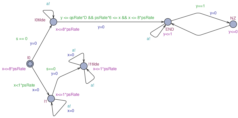
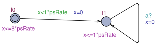
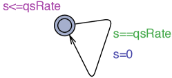
Figure 5: Uppaal Models for ${\cal B}$ of Fig. 4.

6 Conclusion and Future Work

In this paper we have proved some new results for predictability of events’ occurrences for timed automata. We also contributed a new and simpler definition of bounded predictability for finite automata. The natural extensions of our work are as follows:

• in [10], P. Bouyer, F. Chevalier and D. D’Souza proposed an algorithm to decide the existence of a diagnoser with fixed resources (number of clocks and constants). The very same question arises for the existence of a predictor in timed systems.

• dynamic observers [17] have been proposed in the context of fault diagnosis and opacity [18]; in [19] it is shown how to compute a most permissive observer that ensures diagnosability (or opacity [20]) and also how to compute an optimal observer [21] (w.r.t. to a given criterion). We can define the same problems for predictability.

• given the similarities between the fault diagnosis and predictability problems, it would be interesting to state these two problems in a similar and unified way and design an algorithm that can solve the unified version.

Appendix 0.A Proof of Theorem 4.1

Proof

if Part. Assume there exists a $0$-predictor $P$ for $A$ and Equation (3) does not hold. Then $\forall n,\exists w\in L_{f},\forall t\in\overline{w}$, $\mathbf{P}(t)$ does not hold. Let $t=w^{-0}=w$. As $\mathbf{P}(t)$ does not hold: $\exists u\in L_{\neg f},\exists v\in{\cal L}^{*}(A)/u,\boldsymbol{\pi}(u)=\boldsymbol{\pi}(t)\wedge|v|\geq n$ but $|v|_{f}=0$. Assume we have $n\geq|Q|$, the number of states of $A$. Then $v$ has a cycle (pumping Lemma) and can be written $v=x.y.z$ with $|x.y^{j}.z|_{f}=0,x.y^{j}.z\in{\cal L}^{*}(A)/u,\forall j\geq 0$ and thus we can build $v^{\prime}=x.y^{\omega}\in{\cal L}(A)^{\omega}/u$ s.t. $|v^{\prime}|_{f}=0$. It follows that $u\ v^{\prime}\in{\cal L}^{\omega}_{\neg f}$. We have: 1) $w\in L^{-0}_{f}$, 2) $w^{\prime}\in L^{\omega}_{\neg f}$. Moreover $\boldsymbol{\pi}(w^{-0})=\boldsymbol{\pi}(t)$ and $P(\boldsymbol{\pi}(w^{-0}))=1$ because $P$ is a $0$-predictor. But $\boldsymbol{\pi}(t)=\boldsymbol{\pi}(u)$ and $u\in\overline{L^{\omega}_{\neg p}}$ which entails $P(\boldsymbol{\pi}(u))=0$ which is a contradiction.

Only if. Assume Equation (3) holds. Define the mapping $P$ as follows:

• $\forall w\in L^{-0}_{f},P(\boldsymbol{\pi}(w))=1$ and

• $\forall w\in\overline{L^{\omega}_{\neg p}}$, $P(\boldsymbol{\pi}(w))=0$.

We can show that $P$ is a $0$-predictor i.e., it is well-defined. On the contrary assume there exists $r=\boldsymbol{\pi}(w_{1})$ with $w_{1}\in L^{-0}_{f}$ and $r=\boldsymbol{\pi}(w_{2})$ with $w_{2}\in\overline{L^{\omega}_{\neg p}}$. We can show that Equation (3) cannot hold which is a contradiction. Take $n\in\mathbb{N}$. $w_{1}\in L^{-0}_{f}=L_{f}$ and, by Equation (3), there must exist $t\in\overline{w_{1}}$ s.t. $\mathbf{P}(t)$ holds. But we can exhibit two words $u\in L_{\neg p}$ and $v\in{\cal L}^{*}(A)/u$ that falsify $\mathbf{P}(t)$. $t\in\overline{w_{1}}$. As $\boldsymbol{\pi}(w_{1})=\boldsymbol{\pi}(w_{2})$, there exists $w^{\prime}_{2}\in\overline{w_{2}}$ s.t. $\boldsymbol{\pi}(t)=\boldsymbol{\pi}(w^{\prime}_{2})$. $w^{\prime}_{2}\in\overline{L^{\omega}_{f}}$ because $w_{2}\in\overline{L^{\omega}_{f}}$. Take $u=w^{\prime}_{2}$ and $v\in L_{\neg f}/w^{\prime}_{2}$ with $|v|\geq n$ (exists as $w^{\prime}_{2}\in\overline{L^{\omega}_{f}}$). We have $\boldsymbol{\pi}(u)=\boldsymbol{\pi}(t)$, $v\in{\cal L}^{*}(A)/u$, $|v|\geq n$ but $|v|_{f}=0$ which contradicts Equation (3). ∎

Appendix 0.B Proof of Lemma 2

Proof

If. Assume $\boldsymbol{\pi}(L^{-\Delta}_{f})\cap\boldsymbol{\pi}(\overline{L^{\omega}_{\neg f}})\neq\varnothing$. Let $w\in\boldsymbol{\pi}(L^{-\Delta}_{f})\cap\boldsymbol{\pi}(\overline{L^{\omega}_{\neg f}})$. Then $w=\boldsymbol{\pi}(w_{1})=\boldsymbol{\pi}(w_{2})$ with $w_{1}\in L^{-\Delta}_{f}$ and $w_{2}\in\overline{L^{\omega}_{\neg f}}$. Moreover there exists some $w^{\prime}_{2}\in L^{\omega}_{\neg f}$ such that $w_{2}.w^{\prime}_{2}\in L^{\omega}_{\neg f}$. It follows that $\boldsymbol{\pi}(w_{2}.w^{\prime}_{2})$ is an infinite timed word because by assumption every infinite timed has an infinite number of events in $\Sigma_{o}$. By definition of $L^{\omega,-\Delta}_{f}$, $w_{1}.w^{\prime}_{2}\in L^{\omega,-\Delta}_{f}$. Moreover ${\textit{Dur}}(w_{1})={\textit{Dur}}(w_{2})$ and $\boldsymbol{\pi}(w_{1})=\boldsymbol{\pi}(w_{2})$ and thus $\boldsymbol{\pi}(w_{1}.w^{\prime}_{2})=\boldsymbol{\pi}(w_{1}).\boldsymbol{\pi}(w^{\prime}_{2})=\boldsymbol{\pi}(w_{2}.w^{\prime}_{2})$. This entails $\boldsymbol{\pi}(L^{\omega,-\Delta}_{f})\cap\boldsymbol{\pi}(L^{\omega}_{\neg f})\neq\varnothing$.

Only If. Now assume $w\in\boldsymbol{\pi}(L^{\omega,-\Delta}_{f})\cap\boldsymbol{\pi}(L^{\omega}_{\neg f})\neq\varnothing$. We have $w=\boldsymbol{\pi}(w_{1}.w^{\prime}_{1})=\boldsymbol{\pi}(w_{2})$ with $w_{1}\in L^{-\Delta}_{f}$, $w_{2}\in L^{\omega}_{\neg f}$. Let $w^{\prime}_{2}$ be a prefix of $w_{2}$ such that $\boldsymbol{\pi}(w^{\prime}_{2})=\boldsymbol{\pi}(w_{1})$ (such a prefix exists because $\boldsymbol{\pi}(w_{1}.w^{\prime}_{1})=\boldsymbol{\pi}(w_{2})$.) Then $w^{\prime}_{2}\in\overline{L^{\omega}_{\neg f}}$ and $w_{1}\in L^{-\Delta}_{f}$ and $\boldsymbol{\pi}(w^{\prime}_{2})=\boldsymbol{\pi}(w_{1})$ which entails that $\boldsymbol{\pi}(L^{-\Delta}_{f})\cap\boldsymbol{\pi}(\overline{L^{\omega}_{\neg f}})\neq\varnothing$. ∎

Appendix 0.C Proof of Lemma 3

Proof

$\supseteq$ Let $w\in{\cal L}^{\omega}(A_{1}(\Delta)\times A_{2})={\cal L}^{\omega}(A_{1}(\Delta))\cap{\cal L}^{\omega}(A_{2})$. Then $w=\boldsymbol{\pi}(\textit{tr}(\rho_{1}))$ with $\rho_{1}\in\textit{Runs}^{\omega}(A_{1}(\Delta))$ and $w=\boldsymbol{\pi}(\textit{tr}(\rho_{2}))$ with $\rho_{2}\in\textit{Runs}^{\omega}(A_{2})$. We can write $\textit{tr}(\rho_{1})=w_{1}.w^{\prime}_{1}.w^{\prime\prime}_{1}$ with $w_{1}\in L^{-\Delta}_{f}$, ${\textit{Dur}}(w^{\prime}_{1})\leq\Delta$ and $w^{\prime\prime}_{1}\in(\mathbb{R}_{\geq 0}\times\Sigma_{o})^{\omega}$ by construction of $A_{1}$ and its accepting condition. It follows that $w\in\boldsymbol{\pi}(L^{\omega,-\Delta}_{f})\cap\boldsymbol{\pi}(L^{\omega}_{\neg f})$.

$\subseteq$ Let $w\in\boldsymbol{\pi}(L^{\omega,-\Delta}_{f})\cap\boldsymbol{\pi}(L^{\omega}_{\neg f})$. Fig. 6 depicts the following proof. We can write $w=\boldsymbol{\pi}(w_{1}.w^{+}_{1})$ with $w_{1}\in L^{-\Delta}_{f}$, $w^{+}_{1}\in(\mathbb{R}_{\geq 0}\times\Sigma_{o})^{\omega}$. We also have $w=\boldsymbol{\pi}(w_{2}.w^{+}_{2})$ for some $w_{2}.w^{+}_{2}\in L^{\omega}_{\neg f}$ and such that $\boldsymbol{\pi}(w_{1})=\boldsymbol{\pi}(w_{2})$ and $\boldsymbol{\pi}(w^{+}_{1})=\boldsymbol{\pi}(w^{+}_{2})$. Note also that $\boldsymbol{\pi}(w_{2}.w^{+}_{2})\in{\cal L}^{\omega}(A_{2})$ because we assume every infinite timed word has an infinite number of $\Sigma_{o}$ actions.

Figure 6: Proof of Lemma 3, $\subseteq$.

As $w_{1}\in L^{-\Delta}_{f}$, we can split $w^{+}_{1}$ into $w^{+}_{1}=w^{\prime}_{1}.w^{\prime\prime}_{1}$ with ${\textit{Dur}}(w^{\prime}_{1})\leq\Delta$. We can split $w^{+}_{2}$ accordingly such that $w^{+}_{2}=w^{\prime}_{2}.w^{\prime\prime}_{2}$ and $\boldsymbol{\pi}(w^{\prime}_{2})=\boldsymbol{\pi}(w^{\prime}_{1})$ and $\boldsymbol{\pi}(w^{\prime\prime}_{2})=\boldsymbol{\pi}(w^{\prime\prime}_{1})$ and ${\textit{Dur}}(w^{\prime}_{2})={\textit{Dur}}(w^{\prime}_{1})\leq\Delta$. Moreover $w_{1}.w^{\prime}_{2}$ can be generated in $A_{1}(\Delta)$ as follows: start with $w_{1}$, after $w_{1}$ switch to the twin copy and reset $y$ and generate $w^{\prime}_{2}$. By playing $w^{\prime}_{1}$ in the original copy of $A$ in $A_{1}(\Delta)$ we reach a state $(l^{\prime},v)$ where $f$ is enabled: there is a transition $(l^{\prime},g,f,R,l_{f})\in E$ such that $v\models g$. By construction of $A_{1}(\Delta)$, playing $w^{\prime}_{2}$ in the twin copy in $A_{1}(\Delta)$ we reach an equivalent state $(\tilde{l}^{\prime},v)$ and a twin transition $(\tilde{l}^{\prime},g\wedge y\leq\Delta,\varepsilon,\{y\},\text{END})$. As ${\textit{Dur}}(w^{\prime}_{2})\leq\Delta$, we must have $y\leq\Delta$ and this twin transition can be fired and END is reachable. We can subsequently read $w^{\prime\prime}_{2}$ in $A_{1}(\Delta)$. It follows that $\boldsymbol{\pi}(w_{1}.w^{+}_{2})\in{\cal L}^{\omega}(A_{1}(\Delta))$ and $w\in{\cal L}^{\omega}(A_{1}(\Delta)\times A_{2})$. ∎

References

- [1] Sampath, M., Sengupta, R., Lafortune, S., Sinnamohideen, K., Teneketzis, D.: Diagnosability of discrete event systems. IEEE Transactions on Automatic Control 40(9) (September 1995)
- [2] Yoo, T.S., Lafortune, S.: Polynomial-time verification of diagnosability of partially-observed discrete-event systems. IEEE Transactions on Automatic Control 47(9) (September 2002) 1491–1495
- [3] Jiang, S., Huang, Z., Chandra, V., Kumar, R.: A polynomial algorithm for testing diagnosability of discrete event systems. IEEE Transactions on Automatic Control 46(8) (August 2001)
- [4] Alur, R., Dill, D.: A theory of timed automata. Theoretical Computer Science 126 (1994) 183–235
- [5] Genc, S., Lafortune, S.: Predictability of event occurrences in partially-observed discrete-event systems. Automatica 45(2) (2009) 301–311
- [6] Genc, S., Lafortune, S.: Predictability in discrete-event systems under partial observation. In: IFAC Symposium on Fault Detection, Supervision and Safety of Techical Processes, Beijing, China, IEEE (2006)
- [7] Jéron, T., Marchand, H., Genc, S., Lafortune, S.: Predictability of sequence patterns in discrete event systems. In: IFAC World Congress, Seoul, Korea (July 2008) 537–453
- [8] Brandán Briones, L., Madalinski, A.: Bounded predictability for faulty discrete event systems. In: 30th International Conference of the Chilean Computer Science Society (SCCC-11). (2011)
- [9] Tripakis, S.: Fault diagnosis for timed automata. In Damm, W., Olderog, E.R., eds.: Proceedings of the International Conference on Formal Techniques in Real Time and Fault Tolerant Systems (FTRTFT’02). Volume 2469 of LNCS., Springer (2002) 205–224
- [10] Bouyer, P., Chevalier, F., D’Souza, D.: Fault diagnosis using timed automata. In Sassone, V., ed.: FoSSaCS. Volume 3441 of LNCS., Springer (2005) 219–233
- [11] Larsen, K.G., Pettersson, P., Yi, W.: Uppaal in a nutshell. STTT 1(1-2) (1997) 134–152
- [12] Behrmann, G., Fehnker, A., Hune, T., Larsen, K.G., Pettersson, P., Romijn, J., Vaandrager, F.W.: Minimum-cost reachability for priced timed automata. In Benedetto, M.D.D., Sangiovanni-Vincentelli, A.L., eds.: HSCC. Volume 2034 of LNCS., Springer (2001) 147–161
- [13] Courcoubetis, C., Yannakakis, M.: Minimum and maximum delay problems in real-time systems. Formal Methods in System Design 1(4) (1992) 385–415
- [14] Cormen, T.H., Leiserson, C.E., Rivest, R.L., Stein, C.: Introduction to Algorithms (3. ed.). MIT Press (2009)
- [15] Wulf, M.D., Doyen, L., Raskin, J.F.: Almost asap semantics: From timed models to timed implementations. In Alur, R., Pappas, G.J., eds.: HSCC. Volume 2993 of LNCS., Springer (2004) 296–310
- [16] Cassez, F., Henzinger, T.A., Raskin, J.F.: A Comparison of Control Problems for Timed and Hybrid Systems. In: Proc. of the Workshop on Hybrid Systems: Computation and Control (HSCC’02). Volume 2289 of LNCS., Springer (March 2002) 134–148
- [17] Cassez, F., Tripakis, S.: Fault diagnosis with static and dynamic diagnosers. Fundamenta Informaticae 88(4) (November 2008) 497–540
- [18] Cassez, F., Dubreil, J., Marchand, H.: Synthesis of opaque systems with static and dynamic masks. Formal Methods in System Design 40(1) (2012) 88–115
- [19] Cassez, F., Tripakis, S., Altisen, K.: Sensor minimization problems with static or dynamic observers for fault diagnosis. In: 7th Int. Conf. on Application of Concurrency to System Design (ACSD’07), IEEE Computer Society (2007) 90–99
- [20] Cassez, F., Dubreil, J., Marchand, H.: Dynamic observers for the synthesis of opaque systems. In Liu, Z., Ravn, A.P., eds.: ATVA. Volume 5799 of LNCS., Springer (2009) 352–367
- [21] Cassez, F., Tripakis, S., Altisen, K.: Synthesis of optimal-cost dynamic observers for fault diagnosis of discrete-event systems. In: Proceedings of the 1st IEEE & IFIP International Symposium on Theoretical Aspects of Software Engineering (TASE’07), IEEE Computer Society (2007) 316–325