Closed Light Paths in Equiangular Spiral Disks

Abstract

A new type of deformation for microscopic laser disks, the equiangular spiral deformation is proposed. First a short review of the geometry of light paths in equiangular spirals in the language of real two-dimensional geometric calculus is given. Second, the constituting equations for closed paths inside equiangular spirals are derived. Third, their numerical solution is performed and found to yield two generic types of closed light paths. Degenerate closed paths that exist over large intervals of the deformation parameter, and nondegenerate closed paths which only exist over relatively small deformation parameter intervals spanning less than 1% of the nondegenerate intervals. Fourth, amongst the nondegenerate paths a stable asymmetric bow-tie shaped light trajectory was found.

1 Introduction

Quantum cascade laser disks deformed into flattened quadrupoles [1] or ovals [2, 3, 4] have been shown to exhibit a quasi-exponential increase of the collected emitted power with increasing deformation. At the same time such micro-lasers provide a dramatic increase in directionality. In the favourable directions a power increase of up to three orders was obtained. The micro-disks are manufactured from high refractive index ($n_{r}\approx 3.3$) materials like as InGaAs/InAlAs systems. At small deformations chaotic whispering gallery modes dominate, being replaced by stable symmetric bow-tie resonator modes at higher deformations [1].

Theoretical considerations show that deformation from circularity causes the wave equation to be inseparable and the solution can no longer be indexed by quantum numbers. A new theoretical approach providing better physical understanding is the study of the short wavelength limit of the problem, i.e., ray optics for the Helmholtz equation, thus developping a systematic understanding with semiclassical methods. Imposing in a first step a mirror boundary with unit reflectivity makes the Helmholtz equation become identical to the Schrödinger equation and in the short wavelength limit then Newtonian mechanics becomes applicable. The large shifts in resonance frequencies compared to the resonance spacings caused by the deformations prohibit the use of standard perturbation techniques as well [1].

This paper therefore examines the propagation of rays like in a billiard, obeying the law of specular reflection at the boundary.

With respect to the desired shape of a micro-disk, a circular disk, emitting light through frustrated total reflection is rather inefficient and isotropic [4]. This insight paved the way towards breaking the rotational symmetry. The flattened quadrupole (oval) disks greatly improved emission and directionality, yet “a further improvement may be expected if the remaining symmetries of reflection of the oval prototype are broken in an appropriate way. [4]”

I therefore suggest to consider a new type of basic deformation of circular disks: equiangular spiral deformations. As for a circle, radius and tangent always enclose an angle of $\pi/2$. Increasing this angle by a constant angle $\delta$ deforms the circle to an equiangular spiral.

In this paper I first describe this deformation in the language of two-dimensional geometric calculus [5], which is equally suited to describing the classical hardwall shortwave limit [6], the application of semiclassical methods [7] and the full quantum theory [8, 9]. This approach is further motivated by the fact that geometric calculus proves to be “a unified language for mathematics and physics. [10]”

After showing how geometric products of vectors describe rotations and reflections (see also [11]), I derive how the law of sinuses in the language of geometric calculus relates two successive reflections with each other. A detailed investigation of the consequences of this for classical ray propagation in equiangular spirals has already been carried out in [7]. The present work only briefly discusses some new results on ray propagation and equiangular spiral geometry. It is then argued from a classical point of view that for the occurance of closed paths the gap (comp. figure 1) should have unit reflectivity as well. Then two-dimensional geometric calculus is used for the general derivation of the constituting equations of closed paths in equiangular sprials. These constituting equations are first stated in terms of (bivector parts of) products of rotations (rotors) and radii of points of reflections. After that the explicite forms useful for numerical calculations are given.

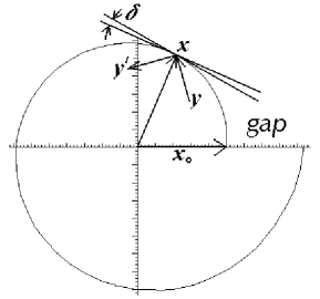
Figure 1: An equiangular spiral with deformation parameter $\delta=0.1$. The tangent at x and a line perpendicular to the radius vector x  are shown. They enclose the angle $\delta$.

The section on numerical results first briefly describes the numerical algorithm. This is followed by a detailed discussion of a set of basic closed paths with up to nine reflections on the equiangular spiral boundary plus one reflection at the gap. A major result is the general presence of degenerate modes with vertical reflections at the gap, whereas nondegenerate modes with angles of reflection less than $\pi/2$ appear to exist only for very special values of the deformation parameter $\delta$. Amongst the nondegenerate paths, the path with $n=3$ reflections on the equiangular spiral boundary plus one reflection at the gap proves to be a stable asymmetric bow-tie shaped light trajectory. Stability is shown for a narrow subinterval of the $n=3$ nondegeneracy $\delta$-interval.

2 Geometry of light paths in equiangular spiral disks

In this section I will only summarize and slightly enhance the results of previous work [7] without repeating most of the proves.

2.1 Equiangular spiral described through geometric calculus

The arena of geometry I will be dealing with is a real two dimensional Euclidean vector space $\mathcal{E}_{2}$ representing a plane and its real geometric algebra $\mathcal{G}_{2}$. Fundamental for the notion of vector in geometric calculus is the associative geometric product of two vectors a, b:

$$\mbox{\bf a}\mbox{\bf b}=<\mbox{\bf a}\mbox{\bf b}>+<\mbox{\bf a}\mbox{\bf b}>_{2}=\mbox{\bf a}\cdot\mbox{\bf b}+\mbox{\bf a}\wedge\mbox{\bf b}$$

composed of the scalar inner product $<\mbox{\bf a}\mbox{\bf b}>=\mbox{\bf a}\cdot\mbox{\bf b}$ and the outer product $\mbox{\bf a}\wedge\mbox{\bf b}$. The latter simply represents the oriented area swept out by b, as it is displaced parallel along a. It is also called a bivector $<\mbox{\bf a}\mbox{\bf b}>_{2}=\mbox{\bf a}\wedge\mbox{\bf b}$ or in this case pseudoscalar, because its rank two is maximal in $\mathcal{G}_{2}$.

The product of two vectors forms a spinor. With the help of the oriented unit area element ${\mathbf{i}}\in\mathcal{G}_{2}$ it can be written in exponential form

ab $$= a\,b\,\,\exp({\mathbf{i}}\Phi)$$ (1)

$$= a\,b\,\,(\cos\Phi+{\mathbf{i}}\sin\Phi)$$

$$a = \sqrt{\mbox{\bf a}\mbox{\bf a}}$$

with ${\mathbf{i}}^{2}=-1$.

For the special case that both a and b are unit vectors $(a=b=1)$

$$R_{ab}=\mbox{\bf a}\mbox{\bf b}=\exp({\mathbf{i}}\Phi)$$ (2)

can be used to describe the rotation of a into b:

$$\mbox{\bf a}R_{ab}=\mbox{\bf b}.$$ (3)

This is the reason why $R_{ab}$ is called a rotor.

An equiangular spiral may now be described as

$$\mbox{\bf x}=\mbox{{x}}_{0}\exp({\mathbf{i}}\Phi+t\Phi)$$ (4)

with $t=\mbox{const.}\in\mathbf{R}$, $t>0$, and $\Phi\in[0,2\pi[$. The second term in the sum of the exponential describes the radial increase compared to a circle with radius $x_{0}$.

It can be shown that the tangent $\partial_{\Phi}\mbox{\bf x}$ at any point x has relative to the direction of the vector x the constant angle

$$\frac{\pi}{2}+\delta\,\,\,\mbox{ with }\,\,\,\delta=\arctan t=\tan^{-1}t.$$ (5)

2.2 Reflections inside an equiangular spiral

A single reflection of a classical light ray as pictured in figure 1 propagating in the direction y takes the simple product from

$$\mbox{\bf y}^{\prime}=R^{{\dagger}}{}(-\delta)(-\mbox{{\^{x}}}\mbox{\bf y}\mbox{{\^{x}}})R(-\delta)\stackrel{{\scriptstyle\mbox{2-dim.}}}{{=}}-\mbox{{\^{x}}}\mbox{\bf y}\mbox{{\^{x}}}R(-2\delta)$$ (6)

with $\mbox{{\^{x}}}=\mbox{\bf x}/x$, the rotor $R(-\delta)=\exp(-\mathbf{i}\delta)$, and its reverse (comp. [5], p. 5) $R^{{\dagger}}{}(-\delta)=\exp(\mathbf{i}\delta)$. The inner bracket $(-\mbox{{\^{x}}}\mbox{\bf y}\mbox{{\^{x}}})$ simply represents a reflection at a circle with radius vector x, which due to Eq. (5) is followed by a clockwise rotation by the angle of $2\delta$. The anticommutativity of the unit plane area element bivector i with any vector in its plane $\mbox{\bf x}\mathbf{i}=-\mathbf{i}\mbox{\bf x}$ explaines why $R^{{\dagger}}{}(-\delta)$ becomes $R(-\delta)$ when shifted to the right as on the right side of the second equation in Eq. (6).

In this context it proves uesful to distinguish incidence from the right for which the reflected ray leaves the reflecting equiangular spiral boundary to the left of the radius vector of the point of reflection, i.e., $\Theta^{\prime}=\Theta+2\delta\in[0,\pi/2+\delta[$ (comp. figure 1) and incidence from the left for which the reflected ray leaves to the right of the radius vector, i.e., $\Theta^{\prime}\in[-\pi/2+\delta,0[$.

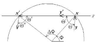
Figure 2: Two successive reflections at an equiangular spiral boundary forming the triangle: origin, x and $\mbox{\bf x}^{\prime}$.

A typical succession of two reflections is shown in figure 2. The origin and the two points of reflection x and $\mbox{\bf x}^{\prime}$ form a triangle. Its three side vectors are related by

$$\mbox{\bf x}^{\prime}=\mbox{\bf x}+(\mbox{\bf x}^{\prime}-\mbox{\bf x}).$$

Hence

$$<(\mbox{\bf x}^{\prime}-\mbox{\bf x})\mbox{\bf x}^{\prime}>_{2}=<(\mbox{\bf x}^{\prime}-\mbox{\bf x})\mbox{\bf x}>_{2},$$ (7)

or equivalently $(\mbox{\bf x}^{\prime}-\mbox{\bf x})\wedge\mbox{\bf x}^{\prime}=(\mbox{\bf x}^{\prime}-\mbox{\bf x})\wedge\mbox{\bf x}$, since the outer product of $\mbox{\bf x}^{\prime}-\mbox{\bf x}$ with itself necessarily vanishes. With the help of Eq. (1) and by dividing Eq. (7) with $\mid\mbox{\bf x}^{\prime}-\mbox{\bf x}\mid$, and with i shows that Eq. (7) is nothing else but the familiar law of sinuses

$$x^{\prime}{}\,\sin\Theta^{\prime\prime}=x\,\sin(\pi-\Theta^{\prime})=x\,\sin\Theta^{\prime}$$ (8)

or simply

$$\sin\Theta^{\prime}-\frac{x^{\prime}}{x}\sin\Theta^{\prime\prime}=0.$$

According to Eq. (4) the ratio of the two radii is $x^{\prime}/x=\exp[t(\Phi^{\prime}-\Phi)]$ and we therefore finally obtain

$$\sin\Theta^{\prime}-\exp(t\Delta\Phi)\sin\Theta^{\prime\prime}=0$$ (9)

with $\Delta\Phi=\Phi^{\prime}-\Phi$.

As the derivation above shows, Eq. (9) holds no matter whether the direction $\Phi=0$ is not intersected by the line segment $\overline{\mbox{\bf x}\mbox{\bf x}^{\prime}}$ as in figure 2 or whether it is intersected.

For right incident rays Eq. (9) can be visualized as in figure 3. The detailed examination of Eq. (9) yields that in general

$$\Theta^{\prime\prime}>\Theta$$

holds for right incident rays and

$$\Theta^{\prime\prime}<\Theta$$

for left incident rays.

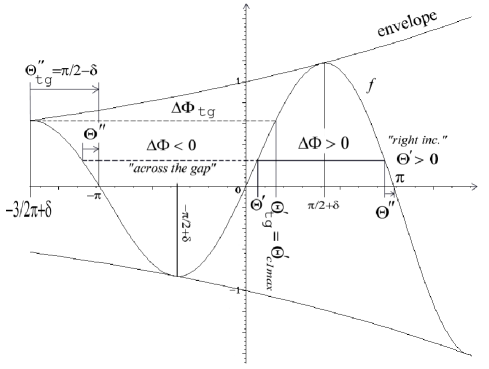
Figure 3: Graphical solution of Eq. (9) for successive reflections of right incident rays. $\Delta\Phi_{tg}$, $\Theta^{\prime}_{tg}$, $\Theta^{\prime}_{c1max}$ are all shown in figure 4, and $f=\exp(t\Theta^{\prime})\sin\Theta^{\prime}$.

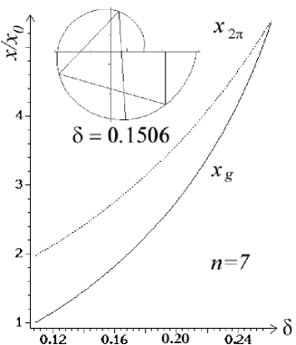
Figure 11: $x_{2\pi}$ and $x_{g}$ for a degenerate closed path with $n=7$ reflections on the equiangular spiral boundary. The inset shows such a closed path for $\delta=0.1506$. The abscissa extends from $\delta_{i}$ to $\delta_{f}$ as given in Table I.

The general development will therefore be that right incident rays follow anticlockwise polygonal paths bending closer and closer to the boundary until they eventually escape. Left incident rays first start to perform clockwise polygonal motions yet bending further and further away from the boundary until they eventually change their state into right incident rays with anticlockwise paths. An illustration corresponding to figure 3 for left incident rays can be found in [7], figure 11.

As for rays leaving the equiangular spiral through the gap, figure 4 shows the range of angles under which this can happen: $\Theta^{\prime}_{c1}{}(\Phi)<\Theta^{\prime}<\Theta^{\prime}_{c2}{}(\Phi)$ where $\Phi$ marks the point of the last reflection on the equiangular spiral boundary and the limiting angles correspond to incidence at $\mathbf{x}_{0}$ and $\mathbf{x}_{2\pi}$, respectively. An example of the numerically calculated dependencies of $\Theta^{\prime}_{c1}{}(\Phi)$ and $\Theta^{\prime}_{c2}{}(\Phi)$ from $\Phi$ is shown in the previously unpublished figure 5. The actual angle and abscissa of escape as shown in figure 4 can be expressed as

$$\Phi_{e}=\Phi-\pi-\Theta^{\prime}\,\,\mbox{and}\,\,x_{e}=x\frac{\sin\Theta^{\prime}}{\sin\Phi_{e}}.$$ (10)

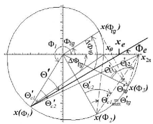
Figure 4: Angles $\Theta^{\prime}_{c1}$ and $\Theta^{\prime}_{c2}$ under which the gap, i.e., $\mbox{{x}}_{0}$ and $\mbox{{x}}_{2\pi}$ , respectively, are seen from various boundary points $\mbox{\bf x}(\Phi_{1})$, $\mbox{\bf x}(\Phi_{2})$, and $\mbox{\bf x}(\Phi_{3})$ on the equiangular spiral . $\overline{\mbox{\bf x}(\Phi_{2})\mbox{{x}}_{0}}$ is part of the tangent at $\mbox{{x}}_{0}$. $\Theta^{\prime}_{tg}$ corresponds to striving tangential incidence at the outside equiangular spiral boundary point $\mbox{\bf x}(\Phi_{tg})$. An escaping ray with angle of escape $\Phi_{e}$ and abscissa of escape $x_{e}$ is shown [comp. Eq. (10)].

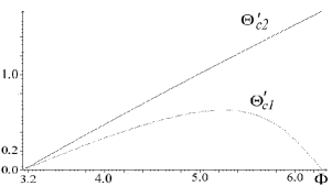
Figure 5: The abscissa $\Phi$ marks the point $\mbox{\bf x}(\Phi)$ of the last reflection on the equiangular spiral boundary. $\Theta^{\prime}_{c1}$ and $\Theta^{\prime}_{c2}$ are the angles under which both ends of the gap, i.e., $\mbox{{x}}_{0}$ and $\mbox{{x}}_{2\pi}$ , respectively, are seen from $\mbox{\bf x}(\Phi)$. The two curves are calculated for $\delta=0.1$.

One of the most interesting results about the geometry of light paths for equiangular spirals is that depending on where one locates a(n isotropic) source of light rays inside an equiangular spiral one may at the initial reflection either have only right incident rays for any ray emitted from the source or one may have both one angular sector with right incident rays and another with left incident rays.

It was found that for sources located inside a certain area, described by a socalled critical equiangular spiral, only right incident rays will be emitted. This critical equiangular spiral has the same origin, and the same $t$ and $\delta$ as the original one, but is rotated anticlockwise by an angle of $\Phi_{0}=\pi/2-\delta$ and shrunk by a factor of $2\sin\delta$. Outside this critical spiral both left and right handed angular sectors exist for the first reflection, delimited by the two tangents to the critical equiangular spiral which pass through the source of the light rays.

An example of a critical equiangular spiral is shown in figure 6 showing the sectors of right and left incidence for a source outside the critical equiangular spiral.

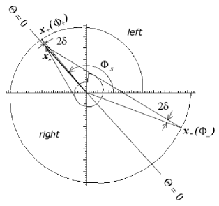
Figure 6: The inner equiangular spiral is the critical curve. For the source $\mbox{{x}}_{s}$ outside it there exists one angular sector with right incidence for the first reflection and another sector with left incidence, respectively. These sectors are delimited by the tangents to the critical equiangular spiral.

A further interesting geometrical property of this critical equiangular spiral is the fact that it can also be constructed as the envelope to the set of once reflected rays, which originate at the origin.

An instructive application of how easy it is to calculate arbitrary directed areas in the frame work of geometrical calculus is provided by the calculation of the oriented area of an equiangular spiral using the following line integral (comp. [6], p. 113):

$$A=\frac{1}{2}\int_{0}^{2\pi}\mbox{\bf x}\,\,\partial_{\Phi}{}\mbox{\bf x}d\Phi$$ (11)

where x depends on $\Phi$ as given in Eq. (4). The derivative $\partial_{\Phi}\mbox{\bf x}$ is simply

$$\partial_{\Phi}\mbox{\bf x}=\mbox{\bf x}_{0}\exp(\mathbf{i}\Phi+t\Phi)(\mathbf{i}+t)=\mbox{\bf x}\mathbf{i}+\mbox{\bf x}t.$$

Inserting this back into (11) we obtain

$$A = \frac{1}{2}\int_{0}^{2\pi}\mbox{\bf x}\wedge(\mbox{\bf x}\mathbf{i})d\Phi+\frac{1}{2}t\int_{0}^{2\pi}\underbrace{\mbox{\bf x}\wedge\mbox{\bf x}}_{=0}d\Phi$$ (12)

$$= \frac{1}{2}\mathbf{i}\int_{0}^{2\pi}x^{2}d\Phi=\frac{1}{2}\mathbf{i}\int_{0}^{2\pi}x^{2}_{0}\exp(2t\Phi)d\Phi$$

$$= \frac{1}{2}x^{2}_{0}\frac{1}{2t}[\exp(2t\Phi)]|^{2\pi}_{0}=\frac{x^{2}_{0}}{4t}[\exp(4\pi t)-1]\mathbf{i}$$

$$= \frac{x^{2}_{2\pi}-x^{2}_{0}}{4t}\mathbf{i}$$

with $\mbox{\bf x}_{2\pi}=\mbox{\bf x}(\Phi=2\pi)$.

The relationship $\mbox{\bf x}\wedge(\mbox{\bf x}\mathbf{i})=x^{2}{}\mathbf{i}$ used here can be understood if one considers that $\mbox{\bf x}\mathbf{i}$ describes according to Eq. (1) an anticlockwise rotation of x by $\pi/2$. x and $\mbox{\bf x}\mathbf{i}$ are therefore perpendicular to each other implying that the scalar part $\mbox{\bf x}\cdot(\mbox{\bf x}\mathbf{i})$ of $\mbox{\bf x}(\mbox{\bf x}\mathbf{i})$ must vanish. The i in Eq. (12) is clearly recognized in its role as oriented unit area element.

Taking into account that

$$(\partial_{\Phi}{}\mbox{\bf x})^{2} = \mbox{\bf x}(\mathbf{i}+t)\mbox{\bf x}(\mathbf{i}+t)$$

$$= \mbox{\bf x}\mbox{\bf x}(-\mathbf{i}+t)(\mathbf{i}+t)$$

$$= \mbox{\bf x}^{2}{}(1+t^{2})$$

we can also calculate the circumference of an equiangular spiral by another line integral

$$U = \int_{0}^{2\pi}[(\partial_{\Phi}{}\mbox{\bf x})^{2}]^{1/2}{}d\Phi=(1+t^{2})^{1/2}{}\int_{0}^{2\pi}x\,d\Phi$$

$$= (1+t^{2})^{1/2}{}\,\,x_{0}\int_{0}^{2\pi}\,\exp(t\Phi)dt$$

$$= \left(\frac{1+t^{2}}{t^{2}}\right)^{1/2}{}x_{0}[\exp(2\pi t)-1]$$

$$\stackrel{{\scriptstyle(\ref{eq:tangle})}}{{=}} \frac{1}{\sin\delta}\,\,g$$

where $g=\mid\mbox{\bf x}_{2\pi}-\mbox{\bf x}_{0}\mid=x_{0}[\exp(2\pi t)-1]$, i.e., the length of the gap of the equiangular spiral as shown in 1.

Since the critical equiangular spiral is just a shrunk (by a factor of $2\sin\delta$) version of the original one we can immediately infer its oriented area and circumference as

$$A_{c}=(\sin\delta)^{2}{}\,A=\frac{1}{2}\sin 2\delta(x_{2\pi}^{2}-x_{0}^{2})\mathbf{i}$$

and

$$U_{c}=2U\sin\delta=2g.$$

The surprising result is therefore that the circumference $U_{c}$ of the critical equiangular spiral measures exactly twice the length $g$ of the gap, i.e., the original spiral’s straight line segment between $\mbox{{x}}_{0}$ and $\mbox{{x}}_{2\pi}$.

This concludes the short discussion of some basic geometrical properties of equiangular spirals and light reflections inside it.

The facts that eventually all light rays inside an equiangular spiral develop into right incident rays and that then the angels of reflection will increase continuously [comp. Eq. (8)] clearly demonstrates the impossibility to arrive at any sort of closed light path provided that the gap is kept “open”. Yet without closed paths an equiangular sprial disk could never qualify as a new disk laser geometry, like the by now familiar oval disks [4, 2]. Possibly the simplest remedy for this might be to “close” the gap by making it 100% reflective as well. That this leads indeed to closed paths will be shown in the next section.

3 Constituting equations for closed paths inside equiangular spirals

An example of a closed path with a total of $n=9$ reflections at the equiangular spiral boundary plus one reflection at the gap is shown figure 7. In general the number of reflections at the equiangular spiral boundary may vary subject to certain restrictions, but as argued at the end of the last section, at least one reflection at the gap will always be present.

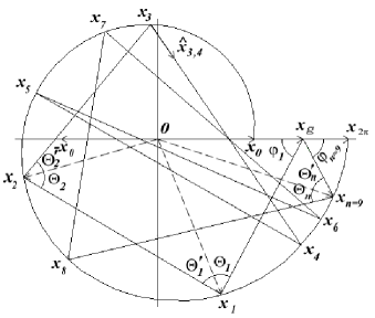
Figure 7: Closed path with $n=9$ (nondegenerate) reflections $\mbox{{x}}_{1}(\Phi_{1}),\ldots,\mbox{{x}}_{n}(\Phi_{n})$ along the equiangular spiral boundary and one reflection at $\mbox{{x}}_{g}$ on the gap $\overline{\mbox{{x}}_{0}\mbox{{x}}_{2\pi}}$.

According to Eq. (4) a point of reflection on the equiangular spiral boundary is given by its position

$$\mbox{\bf x}_{k} = \mbox{\bf x}_{0}\exp(\mathbf{i}\Phi_{k}+t\Phi_{k})$$

$$= \mbox{{\^{x}}}_{k}x_{k}$$

$$= \mbox{{\^{x}}}_{k}x_{0}\exp(t\Phi_{k})$$

where $\mbox{{\^{x}}}_{k}$ is the unit vector in the direction of $\mbox{{x}}_{k}$ and $x_{0}\exp(t\Phi_{k})$ the scalar length of $\mbox{{x}}_{k}$. A useful notation in the following will be the vector of unit length $\mbox{{\^{x}}}_{k,k+1}$ in the direction of $\mbox{{x}}_{k+1}-\mbox{{x}}_{k}$, which is the path a light ray takes on the closed path from $\mbox{{x}}_{k}$ to $\mbox{{x}}_{k+1}$:

$$\mbox{{\^{x}}}_{k,k+1}=\frac{\mbox{{x}}_{k+1}-\mbox{{x}}_{k}}{\mid\mbox{{x}}_{k+1}-\mbox{{x}}_{k}\mid}.$$

We already know from Eq. (6) how $\mbox{{\^{x}}}_{k,k+1}$ and $\mbox{{\^{x}}}_{k-1,k}$ are related with each other by

$$\mbox{{\^{x}}}_{k,k+1} = R^{{\dagger}}{}(-\delta)(-\mbox{{\^{x}}}_{k}\mbox{{\^{x}}}_{k-1,k}\mbox{{\^{x}}}_{k})R(-\delta)$$ (14)

$$\stackrel{{\scriptstyle\mbox{\small 2-dim.}}}{{=}} -\mbox{{\^{x}}}_{k}\mbox{{\^{x}}}_{k-1,k}\mbox{{\^{x}}}_{k}{}R^{2}(-\delta).$$

Equation (14) can be used to successively expand each direction $\mbox{{\^{x}}}_{k,k+1}$ in terms of the “first” direction $\mbox{{\^{x}}}_{g,1}$ of the vector $\mbox{{x}}_{1}-\mbox{{x}}_{g}$, e.g.,

$$\mbox{{\^{x}}}_{1,2}=-\mbox{{\^{x}}}_{1}\mbox{{\^{x}}}_{g,1}\mbox{{\^{x}}}_{1}R(-2\delta)$$ (15)

and

$$\mbox{{\^{x}}}_{2,3} = -\mbox{{\^{x}}}_{2}\mbox{{\^{x}}}_{1,2}\mbox{{\^{x}}}_{2}R(-2\delta)$$

$$= -\mbox{{\^{x}}}_{2}[-\mbox{{\^{x}}}_{1}\mbox{{\^{x}}}_{g,1}\mbox{{\^{x}}}_{1}{}R(-2\delta)]\mbox{{\^{x}}}_{2}R(-2\delta)$$

$$= \mbox{{\^{x}}}_{2}\mbox{{\^{x}}}_{1}\mbox{{\^{x}}}_{g,1}\mbox{{\^{x}}}_{1}\mbox{{\^{x}}}_{2}=R^{{\dagger}}_{12}\mbox{{\^{x}}}_{g,1}R_{12}$$

with the rotor $R_{12}=\mbox{{\^{x}}}_{1}\mbox{{\^{x}}}_{2}=\exp(\mathbf{i}(\Phi_{2}-\Phi_{1}))$ describing an anticlockwise rotation by $\Delta\Phi_{12}=\Phi_{2}-\Phi_{1}$. It is to be noted that the two rotors $R(-2\delta)$ cancelled each other because $R(-2\delta)\mbox{{\^{x}}}_{2}=\mbox{{\^{x}}}_{2}R(2\delta)$, and $R(2\delta)R(-2\delta)=R(2\delta-2\delta)=R(0)=\exp(0\mathbf{i})=1$. The next direction along the closed light path can be expanded as

$$\mbox{{\^{x}}}_{3,4} = -\mbox{{\^{x}}}_{3}\mbox{{\^{x}}}_{2,3}\mbox{{\^{x}}}_{3}R(-2\delta)$$ (17)

$$= -\mbox{{\^{x}}}_{3}R^{{\dagger}}_{12}{}\mbox{{\^{x}}}_{g,1}R_{12}{}\mbox{{\^{x}}}_{3}R(-2\delta).$$

The above expressions for $\mbox{{\^{x}}}_{1,2}$, $\mbox{{\^{x}}}_{2,3}$, and $\mbox{{\^{x}}}_{3,4}$ given in (15),(3), and (17), respectively, are sufficient in order to understand the construction of

$$\mbox{{\^{x}}}_{k,k+1} = R^{{\dagger}}_{k-1k}{}R^{{\dagger}}_{k-3k-2}{}\ldots R^{{\dagger}}_{12}{}\mbox{{\^{x}}}_{g,1}R_{12}$$ (18)

$$\ldots R_{k-3k-2}R_{k-1k}$$

for $k=2l,\mbox{ and }l\in\mathbf{N}$; and

$$\mbox{{\^{x}}}_{k,k+1} = -\mbox{{\^{x}}}_{k}R^{{\dagger}}_{k-2k-1}{}R^{{\dagger}}_{k-4k-3}{}\ldots R^{{\dagger}}_{12}{}\mbox{{\^{x}}}_{g,1}R_{12}$$ (19)

$$\ldots R_{k-4k-3}R_{k-2k-1}\mbox{{\^{x}}}_{k}R(-2\delta)$$

for $k=2l+1,\mbox{ and }l\in\mathbf{N}$. In the very same way as in Eq. (7) we have for each triangle formed by the origin and two successive points of reflection $\mbox{{x}}_{k}$ and $\mbox{{x}}_{k+1}$ on the equiangular spiral

$$<\mbox{{\^{x}}}_{k,k+1}\mbox{{x}}_{k}>_{2}=<\mbox{{\^{x}}}_{k,k+1}\mbox{{x}}_{k+1}>_{2}$$ (20)

Utilizing the expressions (18) and (19) we can proceed now to derive the first set of $n-1$ constituting equations necessary for a closed path. In the following I will first demonstrate the steps involved for $k=1,2$, and 3. With this experience in hand it will then be easy to understand the derivation of the general form for any $k\in\mathbf{N},k<n$. After that I will show how the closing condition yields the last $n$th constituting equation.

Let us therefore begin with Eq. (20) for $k=1$:

$$<\mbox{{\^{x}}}_{1,2}\mbox{{x}}_{1}>_{2}=<\mbox{{\^{x}}}_{1,2}\mbox{{x}}_{2}>_{2}$$

Inserting $\mbox{{x}}_{1}$, $\mbox{{x}}_{2}$ and $\mbox{{\^{x}}}_{1,2}$ according to Eqs. (3) and (15) we obtain

$$<\mbox{{\^{x}}}_{1}\mbox{{\^{x}}}_{g,1}\mbox{{\^{x}}}_{1}R(-2\delta)\mbox{{\^{x}}}_{1}x_{1}>_{2}\hskip 28.45274pt$$

$$=<\mbox{{\^{x}}}_{1}\mbox{{\^{x}}}_{g,1}\mbox{{\^{x}}}_{1}R(-2\delta)\mbox{{\^{x}}}_{2}x_{2}>_{2}.$$

Interchanging the rotor $R(-2\delta)$ with $\mbox{{\^{x}}}_{1}$ and $\mbox{{\^{x}}}_{2}$, respectively, and dividing by $x_{1}$ we get

$$<\mbox{{\^{x}}}_{1}\mbox{{\^{x}}}_{g,1}R(2\delta)>_{2}=\frac{x_{2}}{x_{1}}<\mbox{{\^{x}}}_{1}\mbox{{\^{x}}}_{g,1}\mbox{{\^{x}}}_{1}\mbox{{\^{x}}}_{2}R(2\delta)>_{2}$$ (21)

where we have used the fact that $\mbox{{\^{x}}}_{1}$ is a unit vector, i.e., $\mbox{{\^{x}}}_{1}^{2}=1$. As seen from figure 7 $\mbox{{\^{x}}}_{1}$ and $\mbox{{\^{x}}}_{g,1}$ enclose the angle $\Theta_{1}$ which (because of the left incidence at $\mbox{{x}}_{1}$) will always be negative:

$$\mbox{{\^{x}}}_{1}\mbox{{\^{x}}}_{g,1}=R(\Theta_{1}).$$ (22)

Equation (21) can therefore be rewritten as

$$<R(\Theta_{1})R(2\delta)>_{2} = <R(\Theta_{1}+2\delta)>_{2}$$ (23)

$$= \frac{x_{2}}{x_{1}}<R(\Theta_{1}+2\delta)R_{12}>_{2}$$

since $R(\beta_{1})R(\beta_{2})=R(\beta_{1}+\beta_{2})=R(\beta_{2})R(\beta_{1})$ (additivity of the angles and commutativity of rotations in the same plane with a common center of rotation).

Towards the end of the current section I will proceed to replace the rotors $R$ and the amplitudes $x_{k}$ by their respective exponential expressions. The extraction of the bivector parts $<>_{2}$ as in Eq. (1) will then give the final somewhat unwieldy explicitely transcendental form of the constituting equations necessary for their concrete numerical evaluation.

Next we take Eq. (20) for $k=2$:

$$<\mbox{{\^{x}}}_{2,3}\mbox{{x}}_{2}>_{2}=<\mbox{{\^{x}}}_{2,3}\mbox{{x}}_{3}>_{2}$$

Inserting $\mbox{{x}}_{2}$, $\mbox{{x}}_{3}$ and $\mbox{{\^{x}}}_{2,3}$ according to Eqs. (3) and (3) gives

$$<R^{{\dagger}}_{12}\mbox{{\^{x}}}_{g,1}R_{12}\mbox{{\^{x}}}_{2}>_{2}=\frac{x_{3}}{x_{2}}<R^{{\dagger}}_{12}\mbox{{\^{x}}}_{g,1}R_{12}\mbox{{\^{x}}}_{3}>_{2}.$$ (24)

The only difference to the calculation for $k=1$ is that we need to first express $\mbox{{\^{x}}}_{3}$ in terms of $\mbox{{\^{x}}}_{1}$ using Eq. (3):

$$\mbox{{\^{x}}}_{3}=\mbox{{\^{x}}}_{1}R_{13}.$$ (25)

With the help of Eq. (25) and taking into account that $R_{12}\mbox{{\^{x}}}_{2}=\mbox{{\^{x}}}_{2}R^{{\dagger}}_{12}=\mbox{{\^{x}}}_{2}R_{21}=\mbox{{\^{x}}}_{1}$, and that $R_{12}\mbox{{\^{x}}}_{3}=\mbox{{\^{x}}}_{3}R^{{\dagger}}_{12}$, Eq. (24) attaines the form

$$<R^{{\dagger}}_{12}\mbox{{\^{x}}}_{g,1}\mbox{{\^{x}}}_{1}>_{2}=\frac{x_{3}}{x_{2}}<R^{{\dagger}}_{12}\mbox{{\^{x}}}_{g,1}\mbox{{\^{x}}}_{1}R_{13}R^{{\dagger}}_{12}>_{2}.$$ (26)

The product of the rotors $R_{13}R^{{\dagger}}_{12}$ means first to rotate a vector anticlockwise by $\Phi_{3}-\Phi_{1}$ and then to rotate it back clockwise by $\Phi_{2}-\Phi_{1}$:

$$R_{13}R^{{\dagger}}_{12}=\mbox{{\^{x}}}_{1}\mbox{{\^{x}}}_{3}\mbox{{\^{x}}}_{2}\mbox{{\^{x}}}_{1}=\mbox{{\^{x}}}_{1}R_{32}\mbox{{\^{x}}}_{1}=R^{{\dagger}}_{32}=R_{23}.$$ (27)

Equation (26) together with the relations (22) and (27) results therefore in

$$<R(\Theta_{1})R_{12}>_{2}=\frac{x_{3}}{x_{2}}<R(\Theta_{1})R_{12}R^{{\dagger}}_{23}>_{2}$$ (28)

where I have already applied a final reversion to both sides of the equation.

Setting $k=3$ for Eq. (20) gives

$$<\mbox{{\^{x}}}_{3,4}\mbox{{x}}_{3}>_{2}=<\mbox{{\^{x}}}_{3,4}\mbox{{x}}_{4}>_{2}.$$

By inserting $\mbox{{x}}_{3}$, $\mbox{{x}}_{4}$ and $\mbox{{\^{x}}}_{3,4}$ according to (3) and (17) we obtain

$$<\mbox{{\^{x}}}_{3}R^{{\dagger}}_{12}\mbox{{\^{x}}}_{g,1}R_{12}\mbox{{\^{x}}}_{3}R(-2\delta)\mbox{{\^{x}}}_{3}>_{2}\hskip 56.9055pt$$

$$=\frac{x_{4}}{x_{3}}<\mbox{{\^{x}}}_{3}R^{{\dagger}}_{12}\mbox{{\^{x}}}_{g,1}R_{12}\mbox{{\^{x}}}_{3}R(-2\delta)\mbox{{\^{x}}}_{4}>_{2}$$ (29)

Manipulating Eq. (29) according to the by now familiar rules of geometric calculus we arrive at

$$<R(\Theta_{1}+2\delta)R_{12}R^{{\dagger}}_{23}>_{2}\hskip 56.9055pt$$

$$=\frac{x_{4}}{x_{3}}<R(\Theta_{1}+2\delta)R_{12}R^{{\dagger}}_{23}R_{34}>_{2}$$ (30)

The explicite derivations of the first three constituting Eqs. (23), (28) and (30) are in my view sufficient for understanding the general result for arbitrary $k<n$:

$$<R(\Theta_{1}+2\delta)R_{12}R^{{\dagger}}_{23}\ldots R_{k-2k-1}R^{{\dagger}}_{k-1k}>_{2}$$ (31)

$$= \frac{x_{k+1}}{x_{k}}<R(\Theta_{1}+2\delta)R_{12}R^{{\dagger}}_{23}$$

$$\ldots R^{{\dagger}}_{k-1k}R_{kk+1}>_{2}$$

for $k=2l+1,\mbox{ and }l\in\mathbf{N}$; and

$$<R(\Theta_{1})R_{12}R^{{\dagger}}_{23}\ldots R^{{\dagger}}_{k-2k-1}R_{k-1k}>_{2}$$ (32)

$$= \frac{x_{k+1}}{x_{k}}<R(\Theta_{1})R_{12}R^{{\dagger}}_{23}$$

$$\ldots R_{k-1k}R^{{\dagger}}_{kk+1}>_{2}$$

for $k=2l,\mbox{ and }l\in\mathbf{N}$.

With Eqs. (31) and (32) we have already found all $n-1$ constituting equations which describe the light path between the $n$ points of consecutive reflections along the equiangular spiral boundary. Now we must take the last reflection at the gap into account in order to really close the path back into itself. Looking at figure 7 we see that hence closing means $\varphi_{1}=\varphi_{n}$. In order to express this properly one may, e.g., use two triangles, each containing one of these angles or its $\pi-\varphi$ complement: the ones that shall be used here are formed by the origin, $\mbox{{x}}_{g}$ and $\mbox{{x}}_{1}$ or $\mbox{{x}}_{n}$, respectively. Applying the law of sinuses (7) to both triangles we get:

$$<\mbox{{x}}_{1}\mbox{{\^{x}}}_{g,1}>_{2} \stackrel{{\scriptstyle(\ref{eq:sinlaw})}}{{=}} <\mbox{{x}}_{g}\mbox{{\^{x}}}_{g,1}>_{2}$$

$$= x_{g}<\mbox{{\^{x}}}_{0}\mbox{{\^{x}}}_{g,1}>_{2}$$

$$= -x_{g}\mathbf{i}\sin\varphi_{1}$$

and

$$<\mbox{{x}}_{n}\mbox{{\^{x}}}_{n,g}>_{2} \stackrel{{\scriptstyle(\ref{eq:sinlaw})}}{{=}} <\mbox{{x}}_{g}\mbox{{\^{x}}}_{n,g}>_{2}$$

$$= x_{g}<\mbox{{\^{x}}}_{0}\mbox{{\^{x}}}_{n,g}>_{2}$$

$$= x_{g}\mathbf{i}\sin\varphi_{n}.$$

Hence the equality $\varphi_{1}=\varphi_{n}$ has as a consequence

$$-<\mbox{{x}}_{1}\mbox{{\^{x}}}_{g,1}>_{2}=<\mbox{{x}}_{n}\mbox{{\^{x}}}_{n,g}>_{2}.$$ (33)

Now $\mbox{{\^{x}}}_{n,g}$ is the direction of the light ray reflected at $\mbox{{x}}_{n}$, i.e., that according to Eq. (14)

$$\mbox{{\^{x}}}_{n,g}=-\mbox{{\^{x}}}_{n}\mbox{{\^{x}}}_{n-1,n}\mbox{{\^{x}}}_{n}R(-2\delta).$$ (34)

But $\mbox{{\^{x}}}_{n-1,n}$ is already known to us from Eqs. (18) or (19), respectively. For the case that $n-1$ is even we can rewrite Eq. (33) therefore with the help of (34) and (18) as

$$-<\mbox{{\^{x}}}_{1}\mbox{{\^{x}}}_{g,1}>_{2}$$

$$= \frac{x_{n}}{x_{1}}<\mbox{{\^{x}}}_{n}(-\mbox{{\^{x}}}_{n})R^{{\dagger}}_{n-2n-1}\ldots R^{{\dagger}}_{12}\mbox{{\^{x}}}_{g,1}R_{12}$$

$$\ldots R_{n-2n-1}\mbox{{\^{x}}}_{n}R(-2\delta)>_{2}$$

$$= -\frac{x_{n}}{x_{1}}<R^{{\dagger}}_{n-2n-1}\ldots R^{{\dagger}}_{12}\mbox{{\^{x}}}_{g,1}R_{12}$$

$$\ldots R_{n-2n-1}\mbox{{\^{x}}}_{1}R_{1n}R(-2\delta)>_{2}$$

$$= -\frac{x_{n}}{x_{1}}<R^{{\dagger}}_{n-2n-1}\ldots R^{{\dagger}}_{12}\mbox{{\^{x}}}_{g,1}\mbox{{\^{x}}}_{1}R^{{\dagger}}_{12}$$

$$\ldots R^{{\dagger}}_{n-2n-1}R_{1n}R(-2\delta)>_{2}$$

$$= -\frac{x_{n}}{x_{1}}<R^{{\dagger}}_{n-2n-1}\ldots R^{{\dagger}}_{12}R^{{\dagger}}(\Theta_{1})R_{23}$$

$$\ldots R_{n-1n}R^{{\dagger}}(-2\delta)>_{2}$$

where we have used that $\mbox{{\^{x}}}_{n}=\mbox{{\^{x}}}_{1}R_{1n}$, that $\mbox{{\^{x}}}_{g,1}\mbox{{\^{x}}}_{1}=(\mbox{{\^{x}}}_{1}\mbox{{\^{x}}}_{g,1})^{{\dagger}}=R^{{\dagger}}(\Theta_{1})$, and that $R^{{\dagger}}_{12}\ldots R^{{\dagger}}_{n-2n-1}R_{1n}=R_{23}\ldots R_{n-1n}$. Reversing the right side, which swallows up the minus sign and rearranging the rotors we end up with

$$-<R(\Theta_{1})>_{2} = \frac{x_{n}}{x_{1}}<R(\Theta_{1}+2\delta)R_{12}R^{{\dagger}}_{23}R_{34}$$ (35)

$$\ldots R_{n-2n-1}R^{{\dagger}}_{n-1n}>_{2}.$$

In the same way, just using Eq. (19) instead of Eq. (18) we obtain for odd values of $n-1$:

$$-<R(\Theta_{1})>_{2} = \frac{x_{n}}{x_{1}}<R(\Theta_{1})R_{12}R^{{\dagger}}_{23}R_{34}$$ (36)

$$\ldots R^{{\dagger}}_{n-2n-1}R_{n-1n}>_{2}.$$

We may now summarize: for $n$ reflections along the equiangular spiral boundary plus one reflection at the gap we have now established all $n$ constituting equations. That is, $n-1$ constituting equations for $k=1,\ldots,n-1$ of the form (31) and (32) for the odd and even values of $k$, respectively, plus one constituting equation of the form (35) or (36) for $n$ being odd or even, respectively.

In order to finally see what such a system of $n$ constituting equations looks like in explicitely transcendental form which is necessary for the numerical treatment in the next section, I will give here the constituting equations for the example of figure 7 with $n=9$. This explicite form is obtained by inserting the rotors $R$ according to (2) and the amplitudes $x_{k}$ according to (4) and (3), respectively, into Eqs. (31), (32) and (35), and by extracting the $<>_{2}$ bivector parts. In order to simplify the notation I define $\Delta_{ij}=\Phi_{i}-\Phi_{j}$ with $1\leq i,j\leq n$.

$$\sin(\Theta_{1}+2\delta)$$

$$= \exp(-t\Delta_{12})\sin(\Theta_{1}+2\delta-\Delta_{12})$$

$$\sin(\Theta_{1}-\Delta_{12})$$

$$= \exp(-t\Delta_{23})\sin(\Theta_{1}-\Delta_{12}+\Delta_{23})$$

$$\sin(\Theta_{1}+2\delta-\Delta_{12}+\Delta_{23})$$

$$= \exp(-t\Delta_{34})\sin(\Theta_{1}+2\delta-\Delta_{12}+\Delta_{23}-\Delta_{34})$$

$$\sin(\Theta_{1}-\Delta_{12}+\Delta_{23}-\Delta_{34})$$

$$= \exp(-t\Delta_{45})\sin(\Theta_{1}-\Delta_{12}+\Delta_{23}-\Delta_{34}+\Delta_{45})$$

$$\ldots$$

$$\sin(\Theta_{1}-\Delta_{12}+\Delta_{23}-\Delta_{34}+\Delta_{45}-\Delta_{56}$$

$$+\Delta_{67}-\Delta_{78})$$

$$= \exp(-t\Delta_{89})\sin(\Theta_{1}-\Delta_{12}+\Delta_{23}-\Delta_{34}+\Delta_{45}$$

$$-\Delta_{56}+\Delta_{67}-\Delta_{78}+\Delta_{89})$$

$$-\sin\Theta_{1}$$

$$= \exp[-t(\Delta_{12}+\Delta_{23}+\Delta_{34}+\ldots+\Delta_{89})]$$

$$\sin(\Theta_{1}+2\delta-\Delta_{12}+\Delta_{23}-\Delta_{34}+\ldots$$

$$-\Delta_{78}+\Delta_{89})$$

The system of $n$ constituting equations determines the $n$ variables $\Delta_{kk+1}(k=1,\ldots,n-1)$, and $\Theta_{1}$ completely. But as for concrete applications one is of course interested to calculate the angles $\Phi_{k}(k=1,\ldots,n)$ itself and not only their differences. I will therefore derive a relation giving the explicite dependence of $\Phi_{1}$ with respect to $\Delta_{kk+1}(k=1,\ldots,n-1)$, and $\Theta_{1}$.

We start with the relationship $\varphi_{1}=\varphi_{n}$ already referred to on page 7 for the derivation of the $n$th constituting equation. It is equivalent to

$$\exp(\mathbf{i}\varphi_{1})=\exp(\mathbf{i}\varphi_{n}),$$

which may in turn be equivalently expressed according to (2) by the full geometric products of pairs of unit vectors enclosing these angles, i.e

$$(-\mbox{{\^{x}}}_{0})\mbox{{\^{x}}}_{g,1}=\mbox{{\^{x}}}_{g,n}\mbox{{\^{x}}}_{0}.$$ (37)

It was the bivector part of this relationship that led to Eq. (33).

For the case of $n-1$ being even, Eq. (18) allows us to replace $\mbox{{\^{x}}}_{g,1}$ on the left side of (37) by

$$\mbox{{\^{x}}}_{g,1}=R_{12}R_{34}\ldots R_{n-2n-1}\mbox{{\^{x}}}_{n-1,n}R^{{\dagger}}_{n-2n-1}\ldots R^{{\dagger}}_{34}R^{{\dagger}}_{12}.$$ (38)

using Eq. (6) the reflection of $\mbox{{\^{x}}}_{n-1,n}$ at $\mbox{{x}}_{n}$ into $\mbox{{\^{x}}}_{n,g}=-\mbox{{\^{x}}}_{g,n}$ is described by

$$-\mbox{{\^{x}}}_{g,n}=-\mbox{{\^{x}}}_{n}\mbox{{\^{x}}}_{n-1,n}\mbox{{\^{x}}}_{n}R(-2\delta)$$ (39)

Inserting (38) and (39) back into Eq. (37) and multiplying with $-\mbox{{\^{x}}}_{0}$ from the left yields

$$R_{12}R_{34}\ldots R_{n-2n-1}\mbox{{\^{x}}}_{n-1,n}R^{{\dagger}}_{n-2n-1}\ldots R^{{\dagger}}_{34}R^{{\dagger}}_{12}$$

$$= -\mbox{{\^{x}}}_{0}\mbox{{\^{x}}}_{n}\mbox{{\^{x}}}_{n-1,n}\mbox{{\^{x}}}_{n}R(-2\delta)\mbox{{\^{x}}}_{0}$$

$$= -R_{0n}\mbox{{\^{x}}}_{n-1,n}R^{{\dagger}}_{0n}R(2\delta).$$

Reshuffling all rotors to the left of each side of Eq. (3), multiplying with $\mbox{{\^{x}}}_{n-1,n}$ from the right and expressing the negative sign in exponential form as well results in

$$R^{2}_{12}R^{2}_{34}\ldots R^{2}_{n-2n-1}=\exp(\mathbf{i}\pi)R^{2}_{0n}R^{2}(-\delta)$$

or after taking the squareroot in

$$R_{0n}=\pm\exp(\mathbf{i}\frac{\pi}{2})R(\delta)R_{12}R_{34}\ldots R_{n-2n-1}.$$ (41)

Equating the exponentials of (41) up to multiples of $2\pi$ and considering the sign ambiguity we get

$$\Phi_{n}=(2m+1)\frac{\pi}{2}+\delta-\Delta_{12}-\Delta_{34}\ldots-\Delta_{n-1n-2},m\in\mathbf{Z}$$

since

$$R_{0n}=\mbox{{\^{x}}}_{0}\mbox{{\^{x}}}_{n}=\exp{\mathbf{i}\Phi_{n}}.$$

And since $\Phi_{1}=\Phi_{n}+\Delta_{1n}=\Phi_{n}+\sum_{k=1}^{n-1}\Delta_{kk+1}$ we finally obtain

$$\Phi_{1}=(2m+1)\frac{\pi}{2}+\delta+\Delta_{23}+\Delta_{45}+\ldots+\Delta_{n-1n},m\in\mathbf{Z}.$$

A similar calculation for $n-1$ being odd results in the corresponding expression

$$\Phi_{1}=m\pi-\Theta_{1}+\Delta_{23}+\Delta_{45}+\ldots+\Delta_{n-1n},m\in\mathbf{Z}.$$

It is obvious from figure 7 that the $m$ in the above expressions for $\Phi_{1}$ must be chosen such that $\pi<\Phi_{1}<2\pi$.

4 Numerical results

4.1 Remarks about the numerical technique

In order to evaluate the $n$ constituting equations derived in the last section short numercial algorithms were written with MAPLE V using the command fsolve. The highly transcendental character of the equations made it necessary to first “guess” very narrow intervals (e.g., $\pm 10^{-5}$) around one point of the actual solution. In order to do this a light ray tracing algorithm was developped. By applying it repeatedly to a range of initial conditions $({x}_{g},\varphi_{1})$ the resulting $({x}_{g}^{\prime},\varphi_{n})$ after tracing the rays once along a closed path were obtained and the errors $({x}_{g}^{\prime}-{x}_{g},\varphi_{n}-\varphi_{1})$ were plotted. Gradually minimizing these errors yielded the “guessed” range intervals for the application of MAPLE V‘s fsolve with sufficient accuracy.

The curves $x_{g}(\delta)$ and $\varphi_{1}(\delta)$ were then calculated by first finding the exact point of solution (only limited by the digital accuracy chosen for the application of MAPLE V) in the range interval and successive small stepwise variations of $\delta$ starting from the first exact point of solution.

In practice it was much easier to obtain degenerate paths with $\varphi_{1}=\varphi_{n}=\frac{\pi}{2}$ than nondegenerate paths with $0<\varphi_{1}<\frac{\pi}{2}$.

4.2 Degenerate closed paths with $\varphi_{1}=\varphi_{n}=\frac{\pi}{2}$

It is obvious that the simplest closed light path consists of just one vertical line as indicated in the inset of figure 8. As we know, e.g., from Eq. (6), the angle of incidence $\Theta$  and the angle of the reflected ray $\Theta^{\prime}$  relative to the radius vector of the point of reflection are related by

$$\Theta^{\prime}=\Theta+2\delta$$

In this case we have $\Theta<0$ and $\mid\Theta^{\prime}\mid=\mid\Theta\mid$. Hence

$$\Theta^{\prime}=-\Theta=\delta.$$

The location of the point of reflection on the equiangular spiral boundary will obviously be

$$\Phi=\frac{3}{2}\pi+\delta$$

and as shown in figure 8 the abscissa of reflection $x_{g}$ located on the gap will be

$$x_{g}=x_{0}\exp(t\Phi)\sin\delta$$

under the condition that $x_{g}\geq x_{0}$. This will be the case for

$$\delta>\delta_{c}\approx 0.2638158642...\hskip 28.45274pt.$$

$x_{g}$ will become infinite for $\delta\rightarrow\frac{\pi}{2}$.

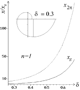
Figure 8: $x_{2\pi}$ and the point of reflection $x_{g}$ on the gap for the degenerate closed path with $n=1$ reflections on the equiangular spiral boundary. An example of such a closed path is shown in the inset for $\delta=0.3$. The abscissa $\delta$ actually extends up to $\delta=\frac{\pi}{2}$ where both $x_{2\pi}$ and $x_{g}{}\,(<x_{2\pi})$ become infinite. The lower limit is given by $x_{g}=x_{0}$.

The next closed path will have the shape of an italic V tilted to the left as in the inset of figure 9. This graph has to be obtained numerically as described in the introduction to this section.

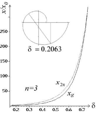
Figure 9: $x_{2\pi}$ and $x_{g}$ for a V-shaped degenerate closed path with $n=3$ reflections on the equiangular spiral boundary. The inset shows such a closed path for $\delta=0.2063$. The abscissa extends from $\delta_{i}$ to $\delta_{f}$ as given in Table I.

The graph in figure 9 shows two curves. The upper one represents $x_{2\pi}/x_{0}$ and the lower one is $x_{g}/x_{0}$. It starts at $\delta_{i}\approx 0.1663186982\,\,(x_{g}=x_{0})$ and ends at $\delta_{f}\approx 0.7453672498$, i.e., the value of $\delta$ for which $x_{g}=x_{2\pi}\approx 330.053788$. For $\delta\notin[\delta_{i},\delta_{f}]$ no such closed path will exist. As we can see in figure 9 the two curves for $x_{g}$ and $x_{2\pi}$ are rather close to each other. Figures 10, 11 and 12 show that this changes as the number of reflections in one cycle increases. Yet the other principal qualitative features like the limits to $\delta$, i.e., $\delta_{i}$ and $\delta_{f}$ with $x_{g}=x_{0}$ and $x_{g}=x_{2\pi}$, respectively, remain valid even for the paths with larger number $n$ of reflections at the equiangular spiral boundary. Table I lists the values of $\delta_{i}$, $\delta_{f}$ and $x_{g}=x_{2\pi}$ for $n=3,5,7$, and 9.

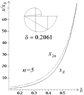
Figure 10: $x_{2\pi}$ and $x_{g}$ for a degenerate closed path with $n=5$ reflections on the equiangular spiral boundary. The inset shows such a closed path for $\delta=0.2061$. The abscissa extends from $\delta_{i}$ to $\delta_{f}$ as given in Table I.

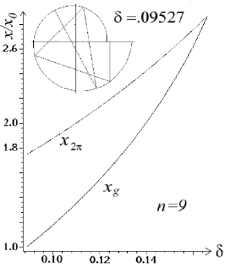
Figure 12: $x_{2\pi}$ and $x_{g}$ for a degenerate closed path with $n=9$ reflections on the equiangular spiral boundary. The inset shows such a closed path for $\delta=9.572\times 10^{-2}$. The abscissa extends from $\delta_{i}$ to $\delta_{f}$ as given in Table I.

Table I: $\delta_{i}$, $\delta_{f}$, and $x_{g}{}(\delta_{f})=x_{2\pi}{}(\delta_{f})$ for $n=3,5,7$, and 9. Values of $x_{g}$ in units of $x_{0}$.

	$n$
	$3$	$5$	$7$	$9$
$\delta_{i}$	0.1663186982	0.1334789387	0.1077909764	0.08875113619
$\delta_{f}$	0.7453672498	0.6062445713	0.2624642501	0.1661601991
$x_{g}=x_{2\pi}$	330.053788	77.97638	5.408937121	2.868332289

Table I and its graphical rendering in figure 13 shows that $\delta_{i}$ and $\delta_{f}$ decrease with incerasing $n$, yet they still overlap each other mutually, except, e.g., for $n=3$ and $n=9$. This means that a kind of mode selection

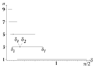
Figure 13: Deformation parameter $\delta$ intervals for the existence of degenerate modes (long $[\delta_{i},\delta_{f}]$ intervals) and nondegenerate modes (short $[\delta_{1},\delta_{2}]$ intervals), respectively. For n=1 no nondegenerate $[\delta_{1},\delta_{2}]$ interval exists.

is possible by choosing sufficiently high or sufficiently low values of $\delta$. E.g., $\delta=0.7$ will select the modes with $n=1$, and $n=3$; or $\delta=0.09$ will select the mode $n=9$, and most likely higher modes.

4.3 Nondegenerate closed paths with $\varphi_{1}=\varphi_{n}<\frac{\pi}{2}$

4.3.1 Nondegenerage closed paths with $n=3$ reflections along the equiangular spiral boundary

In the inset of figure 14 we see that the closed path with $n=3$ distinct nondengenerate points of reflection along the equiangular spiral boundary may be thought of as a splitting up of the degenerate path in figure 9. It has the shape of an asymmetric bowtie. Figure 14 shows three curves: $x_{2\pi}(\delta)$ (top), $x_{g}(\delta)$ (middle) and $\varphi_{1}(\delta)$ (bottom).

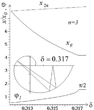
Figure 14: $x_{2\pi}$, the point of reflection on the gap $x_{g}$ and the angle $\varphi_{1}$ (compare figure 7) for the (supposedly) simplest nondegenerate closed path with $n=3$ reflections on the equiangular spiral boundary. It has the shape of an asymmetric bowtie as shown in the inset for $\delta=0.317$. For $\delta>\delta_{2}$, as given in Table II, the closed path becomes degenerate (comp. figure 9) and $\varphi_{1}\equiv\frac{\pi}{2}$.

$x_{g}$ becomes equal to $x_{2\pi}$, if $\delta=\delta_{1}\approx 0.3116739102$. $\varphi_{1}(\delta)$ is a monotonous increasing function which becomes equal to $\pi/2$ at $\delta=\delta_{2}\approx 0.31710313$. For $\delta>\delta_{2}$ only the degenerate closed path with $n=3$ continues to exist. Comparing the intervals $[\delta_{1},\delta_{2}]$ and $[\delta_{i},\delta_{f}]$ of the last section we see that $[\delta_{1},\delta_{2}]\subset[\delta_{i},\delta_{f}]$. Hence both, degenerate and nondegenerate closed paths with $n=3$ reflections on the equiangular spiral boundary coexist for all values $\delta\in[\delta_{1},\delta_{2}]$.

Figure 15 shows the four angles of incidence $\gamma_{k}{}(\delta)=\,\,\mid\Theta_{k}{}(\delta)+\delta\mid\,\,(k=1,2,3)$, and $\gamma_{4}{}(\delta)=\varphi_{4}(\delta)[=\varphi_{1}(\delta)]$ relative to directions perpendicular to the boundary at $\mbox{{x}}_{k}$ $(k=1,2,3)$, and $\mbox{{x}}_{g}$, respectively, for the interval $\delta\in[\delta_{1},\delta_{2}]$. The horizontal line depicts the critical angle of total reflection $\gamma_{c}$, calculated from

$$\sin\gamma_{c}=1/n_{r}$$ (42)

for $n_{r}=3.3$. This is the refractive index of the cascaded InGaAs/InAlAs system used in the well-known symmetric bow-tie micro-disk laser experiments [1]. Figure 15 shows that for a small intervall around $\delta=0.3152\in[\delta_{1},\delta_{2}]$ all four angles of incidence $\gamma_{k},\,\,(k=1,\ldots,4)$ are greater than the critical angle of total reflection $\gamma_{c}$.

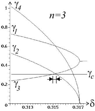
Figure 15: Angles of incidence $\gamma_{k},\,\,(k=1,\ldots,4)$ at $\mbox{{x}}_{1}$, $\mbox{{x}}_{2}$, $\mbox{{x}}_{3}$, and $\mbox{{x}}_{g}$, respectively, for the asymmetric bow-tie shaped closed paths with $n=3$ incidences on the equiangular spiral boundary. Abscissa: $\delta_{1}<\delta<\delta_{2}$ (comp. Table II). Critical angle for total reflection $\sin\gamma_{c}=1/n_{r}$ with $n_{r}=3.3$. Especially marked is the narrow $\delta$-interval for which all $\gamma_{k}>\gamma_{c}$.

This means that light following the $n=3$ nondegenerate closed path trajectories, i.e., the asymmetric bow-tie trajectories as depicted in the inset of figure 14, will stay “forever” trapped within the equiangular spiral micro-disk resonater (neglecting evanescent leakage of tunneling of photons [1]). This will be the case, provided that the deformation parameter $\delta$ is contained in the small intervall around $0.3152$ mentioned above, such that $\gamma_{k}>\gamma_{c},\,\,(k=1,\ldots,4)$. I therefore expect the asymmetric bow-tie mode introduced here to be able to lase.

By virtue of its asymmetry, I expect a further increase in the directionality of the power output, which is to be highest in one of the four directions pertaining to $\mbox{{x}}_{1}$, $\mbox{{x}}_{2}$, $\mbox{{x}}_{3}$ and $\mbox{{x}}_{g}$; compared to the symmetric bow-tie mode with equal power output in all four directions [1].

4.3.2 Nondegenerage closed paths with $n\geq 5$ reflections along the equiangular spiral boundary

Comparing Figs. 14, 16, 17, and 18 shows that the basic features, which have just been explained for the case of $n=3$ nondegenerate reflections continue to persist also for higher values of $n$. Only the transition in the $\varphi_{1}$ curve at $\delta=\delta_{2}$ seems to become more and more abrupt.

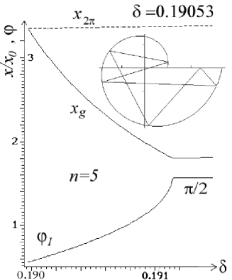
Figure 16: $x_{2\pi}$, the point of reflection on the gap $x_{g}$ and the angle $\varphi_{1}$ (compare figure 7) for the nondegenerate closed path with $n=5$ reflections on the equiangular spiral boundary. An example of such a closed path is shown in the inset for $\delta=0.19053$. For $\delta>\delta_{2}$ (comp. Table II) the path becomes degenerate as in figure 10 and $\varphi_{1}\equiv\frac{\pi}{2}$.

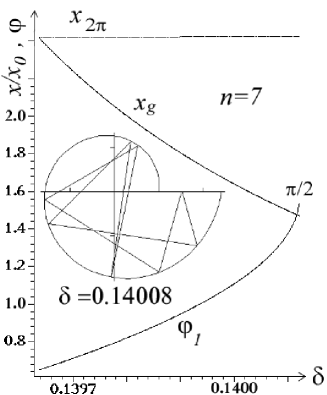
Figure 17: $x_{2\pi}$, the point of reflection on the gap $x_{g}$ and the angle $\varphi_{1}$ (compare figure 7) for the nondegenerate closed path with $n=7$ reflections on the equiangular spiral boundary. An example of such a closed path is shown in the inset for $\delta=0.14008$. For $\delta>\delta_{2}$ (comp. Table II) the path becomes degenerate as in figure 11 and $\varphi_{1}\equiv\frac{\pi}{2}$.

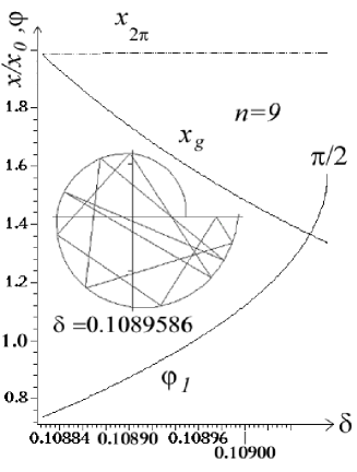
Figure 18: $x_{2\pi}$, the point of reflection on the gap $x_{g}$ and the angle $\varphi_{1}$ (compare figure 7) for the nondegenerate closed path with $n=9$ reflections on the equiangular spiral boundary. An example of such a closed path is shown in the inset for $\delta=0.1089586$. For $\delta>\delta_{2}$ (comp. Table II) the path becomes degenerate as in figure 12 and $\varphi_{1}\equiv\frac{\pi}{2}$.

Table II lists the values of $\delta_{1}$, $x_{g}(\delta_{1})=x_{2\pi}(\delta_{1})$, $\varphi_{1}(\delta_{1})$, $\delta_{2}$, $x_{g}(\delta_{2})$, and $(\delta_{f}-\delta_{i})/(\delta_{2}-\delta_{1})$ for $n=3,5,7$, and 9. For the case of odd $n$ the condititon $x_{g}(\delta_{1})=x_{2\pi}(\delta_{1})$ is equivalent to:

$$\delta_{1}=-\frac{3}{2}\pi+\sum_{k=1}^{(n-1)/2}(\Delta_{2k+1,2k}-\pi)$$

Table II: $\delta_{1}$, $x_{g}(\delta_{1})=x_{2\pi}(\delta_{1})$, $\varphi_{1}(\delta_{1})$, $\delta_{2}$, $x_{g}(\delta_{2})$, and $(\delta_{f}-\delta_{i})/(\delta_{2}-\delta_{1})$ for $n=3,5,7$, and 9. Values of $x_{g}$ in units of $x_{0}$.

	$n$
	3	5	7	9
$\delta_{1}$	0.3116739102	0.1899678060	0.1396366678	0.1088242806
$x_{g}=x_{2\pi}$	7.5706580	3.3473581	2.41840995	1.98670040
$\varphi_{1}(\delta_{1})$	0.551868221	0.561810573	0.648663822	0.734333562
$\delta_{2}$	0.31710313	0.1911406275	0.14012182865	0.10907108189
$x_{g}(\delta_{2})$	4.169707	1.8034054	1.469010	1.3357671
$(\delta_{f}-\delta_{i})/(\delta_{2}-\delta_{1})$	107	403	319	314

The quotient of the length of the degenerate and the nondegenerate $\delta$ intervals in Table II shows that the nondegenerate interval lengths are all less than 1% of the degenerate ones. This partly explaines why the nondegenerate data are more difficult to be calculated in the first place. Table II or figure 13 clearly show that for a given $\delta$ of the nondegenerate modes with $n=3,5,7$, and 9, if at all, only one of these nondegenerate modes will exist. The reason is that the $[\delta_{1},\delta_{2}]$ intervals don‘t overlap. This makes a unique selection amongst the nondegenerate modes possible by simply choosing an appropriate $\delta$ from one of the $[\delta_{1},\delta_{2}]$-intervals, if we neglect the degenerate modes for the moment being.

Table II suggests further that the center points and the lengths of the $[\delta_{1},\delta_{2}]$ intervals decrease continually with increasing $n$, whereas the lengths proportions of the nondegenerate and degenerate $\delta$ intervals pertaining to the same $n$ may continue to be of an order of less than 1%. It is therefore likely that the above suggested unique selection of nondegenerate modes may continue to work for higher $n$ as well.

The fact that all $[\delta_{1},\delta_{2}]$ intervals for nondegenerate modes with $n\geq 5$ have $\delta_{2}<\gamma_{c}(n_{r}=3.3)$ shows that for refractive indices $n_{r}\leq 3.3$ no further stable nondegenerate closed path light trajectories are to be expected. E.g., for $n=5$ the refractive index would in principle have to be as high as $n_{r}=5.26$, in order to create a situation with the possibility of all angles of incidence to be greater than $\gamma_{c}$.

4.4 Existence of nondegenerate modes with even $n$

So far I did not find a numerical solution for a nondegenerate mode with an even number $n$ of reflections along the equiangular spiral boundary, when applying the same techniques as just explained for the case of odd $n$. In the case of odd $n$, a nondegenerate mode may be thought to naturally arise from the splitting up of the corresponding degenerate mode as the branching off of the nondegenerate mode in Figs. 14, and 16 to 18 suggests. Such a branching off into a nondegenerate mode with even $n$ seems unlikely, since no corresponding degenerate mode with an even number of reflections $n$ on the equiangular spiral boundary exists. This consideration may serve as a hint, but seems by itself certainly insufficent to explain the possible nonexistence of nondegenerate modes with even $n$.

5 Conclusion

A new type of deformation, the equiangular spiral deformation of circular disks has been introduced. This deformation simultaneously breaks the symmetry of rotation and contains no remaining symmetries of reflection as in the case of the flattened quadrupoles or ovals [1, 4]. A combination of equiangular spiral and oval deformations may therefore be a promising direction for future investigations.

The real two-dimensional geometric calculus description of equiangular spirals was explained briefly together with a short review of the geometric properties of light ray propagation inside an equiangular spiral.

Then the constituting equations for closed light paths inside an equiangular spiral were derived and their explicite forms fit for numerical solution were given. The numerical solution of these constituting equations showed that there are basically two generic types of closed paths: degenerate paths with vertical incidence at the gap and nondegenerate paths with nonvertical incidence at the gap. The nondegenerate paths were seen to exist only for very specific intervals of the deformation parameter $\delta$ less than a 1% fraction of the permissible $\delta$-intervals of the degenerate closed paths. All interval lenghts, centerpoints and boundaries monotonically decreased with increasing $n$ as shown in figure 13.

It is to be expected that for reflectivities $R$ less than unity, e.g., for dielectrica with $R=(n_{r}-1)^{2}/(n_{r}+1)^{2}$ (Fresnel result for vertical incidence [4, 12]) degenerate modes with vertical incidence at the gap may not be able to lase. Hence a choice of deformation parameter $\delta$ in a $[\delta_{1},\delta_{2}]$ interval specific to some value of $n$ will enable the exclusive selection of the presence of a nondegenerate mode for this particular equiangular spiral disk.

It was further shown that equiangular spirals with deformation parameters contained in a narrow interval around $\delta=0.3152$, exhibit stable asymmetric bow-tie shaped light trajectories, assuming a high refractive index material with $n_{r}=3.3$ as in [1]. Compared to the symmetric bow-tie micro-disk laser [1] an increase in the directionality of the output power in only one preferred direction is to be expected.

In future investigations the Poincaré sections recording the angles of incidence $\gamma=\,\,\mid\Theta+\delta\mid$ versus the polar angle $\Phi$ should be examined for stable orbits above the total reflectivity escape condition (42). This would give sufficiently strong reasons for endeavouring full numeric solutions of the Helmholtz wave equation and for conducting corresponding experiments.

References

- [1] C. Gmachl et al, High-Power Directional Emission from Microlasers with Chaotic Resonators, Science 280 (1998), 1556-1568.
- [2] O. Port (ed), Laser Flashes - Following the Bouncing Light, Business Week, Asian Edition June 15, 73, McGraw-Hill, Singapore, 1998.
- [3] J. U. Nöckel http://www.mpipks-dresden.mpg.de/noeckel/microlasers.html (useful introduction with further interesting links)
- [4] J. U. Nöckel, Microlaser als Photonen-Billard: wie Chaos ans Licht kommt, Phys. Blätter 54 (1998), 927-930.
- [5] D. Hestenes and G. Sobczyk, ”Clifford Algebra to Geometric Calculus, A Unified Language for Mathematics and Physics,” D. Reidel, Dordrecht, 1984.
- [6] D. Hestenes, ”New Foundations for Classical Mechanics,” D. Reidel, Dordrecht, 1987.
- [7] E. Hitzer, The Geometry of Light Paths for Equiangular Spirals, Adv. Appl. Cliff. Alg. 9(2) (1999), 261-286.
- [8] D. Hestenes, ”Space-Time Algebra,” Gordon and Breach, New York, 1966.
- [9] C. J. L. Doran et al, Spacetime Algebra and Electron Physics, in P. W. Hawkes (ed), ”Advances in Imaging and Electron Physics,” Academic, New York, Vol. 95, (1996), 271-386.
- [10] D. Hestenes, A Unified Language for Mathematics and Physics, in 1986 J. S. R. Chisholm (ed), ”Clifford algebras and their appl. in math. phys.,” D. Reidel, Dordrecht, (1986), 1-23.
- [11] S. F. Gull, A. N. Lasenby and C. J. L. Doran, Imaginary Numbers are not Real - the Geometric Algebra of Spacetime, Found. Phys. 23(9), (1993), 1175-1201.
- [12] J. D. Jackson ”Klassische Elektrodynamik,” Walter de Gruyter, New York, 1981.
- [13] Int. Bible. Soc. and BibleGateway, Genesis ch. 1 verses 1 and 3, in ”Bible, New International Version,” IBS, Colorado, 1984, http://bible.gospelcom.net/