The role of the Rashba coupling in spin current of monolayer gapped graphene.

Abstract

In the current work we have investigated the influence of the Rashba spin-orbit coupling on spin-current of a single layer gapped graphene. It was shown that the Rashba coupling has a considerable role in generation of the spin-current of vertical spins in mono-layer graphene. The behavior of the spin-current is determined by density of impurities. It was also shown that the spin-current of the system could increase by increasing the Rashba coupling strength and band-gap of the graphene and the sign of the spin-current could be controlled by the direction of the current-driving electric field.

1 Introduction

Carbon nano materials reveal an interesting polymorphism of different allotropes exhibiting each possible dimensionality: 1) fullerene molecule (0D), 2) nano tubes (1D), 3) graphene and graphite platelets (2D) and 4) diamond (3D) are selected examples.
Since graphene was discovered in 2004 by Geim and his team [1], it has continued to surprise scientists. This is due to some spectacular and fantastic transport properties like the high carrier mobility and universal minimal conductivity at the Dirac point where the valence and conduction bands cross each other [2, 3].
In the presence of spin-orbit couplings, spin polarized states in graphene is a response to an external in-plane electron field. In today’s spintronics, it is a possible key ingredient towards electrical spin control with spin-orbit interaction which has attracted a great attention, such as anomalous Hall effect [4]. Extrinsic spin-orbit interaction (Rashba) that originates from the structure inversion asymmetry (SIA), arises from symmetry breaking generated at interface between graphene and substrate or by external fields [5, 6, 7].
Spin-current control is of crucial importance in electronic devices. Some attempts have been made for applying Rashba interaction to control spin-current. Since Rashba coupling strength in graphene is high relative to other materials, studying the role of this interaction in graphene could remove most of the existing obstacles in spin-current control. As mentioned in previous studies, amount of Rashba interaction in graphene can be at a very high. For example, 0.2 ev which has been reported in [8] can be pointed out.
Depending on graphene’s substrate, strength of the Rashba interaction in graphene can be much higher than its intrinsic spin-orbit interaction. In addition to the spin transport related aspects generated by applying the Rashba interaction, this coupling can be utilized in optical devices as well. As an example, by applying this interaction in two-dimensional electron gas and graphene, controllable blue shift could be obtained in absorption spectrum [9, 10]. Spin-current is an important tool for studying spin related features in graphene and is also important in the development of the graphene quantum computer.
Based on the Tight-Binding model, Soodchomshom has studied the effect of the uniaxial strain in the spin transport through a magnetic barrier of the strained graphene system and shown that graphene has a fantastic potential for applications in nano-mechanical spintronic devices. Strain in graphene will induce the pseudo-potentials at the barrier that can control the spin currents of the junction [11]. Ezawa has considered a nano disk connected with two leads and shown this system acts as a spin filter and can generate a spin-current [12].
In this work, we have considered the influence of Rashba spin-orbit coupling on spin-current of a monolayer gapped graphene. It has been found that the spin-current associated with normal spins is influenced by the Rashba spin-orbit coupling and the energy gap of the system.

2 Model and approach

The low energy charge carriers in graphene are satisfied in a massless Dirac equation. This equation have an isotropic linear energy dispersion near the Dirac points [1]. Meanwhile the Hamiltonian of gapped graphene with Rashba spin-orbit (SO) coupling is [13, 14]

$$\hat{H}=\hat{H}_{G}+\hat{H}_{R}+\hat{H}_{gap}+\hat{V}_{im}.$$ (1)

$\hat{H}_{G}$ is the Dirac Hamiltonian for massless fermions which is given as follows [15, 16]

$$\hat{H}_{G}=-i\gamma\psi^{{\dagger}}(\sigma_{x}\tau_{z}\partial x+\sigma_{y}\partial y)\psi,$$ (2)

$v_{f}$ is the Fermi velocity in graphene, $\gamma=\hbar v_{f}$, $\sigma$ and $\tau$ represent the Pauli matrices where, $\sigma_{z}=\pm 1,\tau_{z}=\pm 1$ denote the Pauli matrice of pseudospin on the A and B sublattices and different Dirac points, respectively.
The second term in equation (1), $H_{R}$, is the Rashba (SO) interaction, and can be expressed as [14, 17]

$$\hat{H}_{R}=\frac{\lambda_{R}}{2}\psi^{{\dagger}}(\sigma_{y}s_{x}-\sigma_{x}\tau_{z}s_{y})\psi,$$ (3)

where $\lambda_{R}$ is the (SO) coupling constant and s denotes Pauli matrix representing the spin of electron. In an ideal graphene sheet, the Dirac electrons are massless and the band structure has no energy gap. Experimentally, it is possible to manipulate an energy gap (from a few to hundreds of meV) in graphene’s band structure, namely a Dirac gap [18, 19, 20]. As a result of the asymmetry in graphene sublattices, A and B, the band gap can have a nonzero value. The last term in $H_{gap}=\tau\Delta\sigma_{z}$ equation (1), referred to mass term, arises from the energy gap $\Delta$ in the spectrum of graphene, that $\tau=1$ $(\tau=-1)$ corresponds to the $K$ ($K^{\prime}$) valley. The last term in equation (1), $\hat{V}_{im}$, is induced due to the short range impurities which can be written as

$$V_{im}(r)=\sum_{j}V\delta({\vec{r}-\vec{r}_{j}}),$$ (4)

where the summation is over the position of impurities. The eigenfunctions of $\hat{H}_{0}=\hat{H}_{G}+\hat{H}_{R}+\hat{H}_{gap}$ are

$$\mid\epsilon_{1}(k)>=\left(\begin{array}[]{cccc}-i\Omega_{1}(k)e^{-2i\varphi}\\ \Omega_{2}(k)e^{-i\varphi}\\ i\Omega_{3}(k)e^{-i\varphi}\\ 1\end{array}\right),$$ (9)

$$\mid\epsilon_{2}(k)>=\left(\begin{array}[]{cccc}i\Omega_{4}(k)e^{-2i\varphi}\\ \Omega_{5}(k)e^{-i\varphi}\\ i\Omega_{3}(k)e^{-i\varphi}\\ 1\end{array}\right),$$ (14)

$$\mid\epsilon_{3}(k)>=\left(\begin{array}[]{cccc}i\Omega_{6}(k)e^{-2i\varphi}\\ \Omega_{7}(k)e^{-i\varphi}\\ -i\Omega_{8}(k)e^{-i\varphi}\\ 1\end{array}\right),$$ (19)

$$\mid\epsilon_{4}(k)>=\left(\begin{array}[]{cccc}-i\Omega_{9}(k)e^{-2i\varphi}\\ \Omega_{10}(k)e^{-i\varphi}\\ -i\Omega_{8}(k)e^{-i\varphi}\\ 1\end{array}\right),$$ (24)

and the corresponding eigenvalues are

$$\epsilon_{1}(k)=-\sqrt{\Delta^{2}+\gamma^{2}k^{2}+\frac{\lambda^{2}}{8}-\frac{\lambda}{8}\Gamma(k)}$$

$$\epsilon_{2}(k)=-\epsilon_{1}(k)$$ (25)

$$\epsilon_{3}(k)=-\sqrt{\Delta^{2}+\gamma^{2}k^{2}+\frac{\lambda^{2}}{8}+\frac{\lambda}{8}\Gamma(k)}$$

$$\epsilon_{4}(k)=-\epsilon_{3}(k)$$

where we have defined

$$\Omega_{1}(k)=-\Lambda_{+}(k)\xi^{(1)}_{+}(k)~{}~{}~{}~{}~{}\Omega_{2}(k)=\xi^{(1)}_{+}(k)$$

$$\Omega_{3}(k)=\Lambda_{-}(k)~{}~{}~{}~{}~{}~{}~{}~{}~{}~{}~{}~{}~{}~{}~{}~{}\Omega_{4}(k)=\Lambda_{+}(k)\xi^{(1)}_{-}(k)$$ (26)

$$\Omega_{5}(k)=\xi^{(1)}_{-}(k)~{}~{}~{}~{}~{}~{}~{}~{}~{}~{}~{}~{}~{}~{}~{}~{}\Omega_{6}(k)=-\Lambda_{-}(k)\xi^{(2)}_{+}(k)$$

$$\Omega_{7}(k)=\xi^{(2)}_{+}(k)~{}~{}~{}~{}~{}~{}~{}~{}~{}~{}~{}~{}~{}~{}~{}~{}\Omega_{8}(k)=\Lambda_{+}(k)$$

$$\Omega_{9}(k)=\Lambda_{-}(k)\xi^{(2)}_{-}(k)~{}~{}~{}~{}~{}~{}~{}~{}\Omega_{10}(k)=\xi^{(2)}_{-}(k)$$

in which $\Gamma(k)=(16\gamma^{2}k^{2}+\lambda^{2})^{1/2}$, $\Lambda_{\pm}(k)=(\pm\lambda+\Gamma(k))/(4\gamma k)$, $\xi^{(1)}_{\pm}(k)=(\Delta\pm\epsilon_{1}(k))/(\gamma k)$ and $\xi^{(2)}_{\pm}(k)=(\Delta\pm\epsilon_{3}(k))/(\gamma k)$.
The transition probabilities between the $|\epsilon_{i}(k)>$ and $|\epsilon_{j}(k^{\prime})>$ states are given by the Fermi’s golden rule,

$$\omega_{ij}(\vec{k},\vec{k^{\prime}})=(2\pi/\hbar)n_{i}|<\vec{k^{\prime}_{j}}|\hat{V_{im}}|\vec{k_{i}}>|^{2}\delta(\epsilon_{i}(\vec{k})-\epsilon_{j}(\vec{k^{\prime}})),~{}~{}~{}~{}~{}(i,j=1,2,3,4).$$ (27)

that $\delta(\epsilon_{i}(\vec{k})-\epsilon_{j}(\vec{k^{\prime}}))\approx\delta({\vec{k}}-{\vec{k^{\prime}}})/\gamma$.
Scattering potential of the impurities is described by the $\hat{V_{im}}$. These are assumed to be distributed randomly with real density $n_{i}$

$$\bar{\omega}_{i}=K\int d\acute{\varphi}\sum_{j}\omega_{ji}(\varphi,\varphi^{\prime}),~{}~{}~{}~{}~{}(i,j=1,2,3,4)$$ (28)

in which $K=(2\pi/\hbar)n_{i}$ and $\varphi$, $\varphi^{\prime}$ are two angles characterizing the direction of $\vec{k}$ and $\vec{k^{\prime}}$ states relative to the $x$ axis respectively. Then the non-equilibrium distribution function of a given $\epsilon_{i}(k)$ energy band can be written as [21]

$$\delta f_{i}=-ev_{i}E(-\partial_{\epsilon}f_{0})[a_{i}(\varphi)cos\theta+b_{i}(\varphi)sin\theta],$$ (29)

in which $E$ is the current driven electric field, $\theta$ is the angle between the $x$ axis and the direction of the electric field and the unknown functions $a_{i}(\varphi)$ and $b_{i}(\varphi)$ can be written as follows

$$a_{i}(\varphi)=a_{0}+\sum_{j=1}a_{cji}\cos(j\varphi)+\sum_{j=1}a_{sji}\sin(j\varphi)$$ (30)

$$b_{i}(\varphi)=b_{0}+\sum_{j=1}b_{cji}\cos(j\varphi)+\sum_{j=1}b_{sji}\sin(j\varphi)$$ (31)

$a_{i}(\varphi)$ and $b_{i}(\varphi)~{}~{}~{}(i=1,2,3,4)$ must satisfy [21]

$$\cos\varphi=\bar{\omega}_{i}a_{i}(\varphi)-K\int d\acute{\varphi}\sum_{j}[\omega_{ij}(\varphi,\varphi^{\prime})a_{j}(\varphi)]$$ (32)

$$\sin\varphi=\bar{\omega}_{i}b_{i}(\varphi)-K\int d\acute{\varphi}\sum_{j}[\omega_{ij}(\varphi,\varphi^{\prime})b_{j}(\varphi)]$$ (33)

it can be easily obtained that the non-vanishing parameters are $a_{c1i}$ and $b_{s1i}$ in which $a_{c_{1i}}=b_{s_{1i}}~{}~{}(i=1-4).$ This can be inferred from the Dirac point approximation in which at this level band energies are appeared to be isotropic in k-space. Meanwhile, these parameters can be obtained through the equations (32)-(33) The non-equilibrium distribution function is then given by

$$\delta f_{i}=-ev_{i}E(-\partial_{\epsilon}f_{0})[a_{c_{1i}}\cos\varphi cos\theta+b_{s_{1i}}\sin\varphi sin\theta]$$ (34)

The spin current operator is defined as [5]

$$J^{s_{i}}_{j}=\{s_{i},\hat{v}_{j}\},$$ (35)

where $\hat{v}_{j}=\hbar^{-1}(\frac{\partial\hat{H}}{\partial k_{j}})~{}~{}(i,j=x,y)$ is the velocity operator. The spin current operator in the basis $e^{(i\vec{k}.\vec{r})}|s\sigma>$ is given as follows,

$$J^{s_{z}}_{x}=\left(\begin{array}[]{cccc}0&\hbar\gamma&0&0\\ \hbar\gamma&0&0&0\\ 0&0&0&-\hbar\gamma\\ 0&0&\hbar\gamma&0\end{array}\right),$$ (36)

$$J^{s_{z}}_{y}=\left(\begin{array}[]{cccc}0&-i\hbar\gamma&0&0\\ i\hbar\gamma&0&0&0\\ 0&0&0&i\hbar\gamma\\ 0&0&-i\hbar\gamma&0\end{array}\right).$$ (37)

Then the average spin currents in x and y directions are given by

$$<J^{s_{i}}_{j}>=\frac{1}{(2\pi)^{2}}\int d^{2}k\sum_{\lambda=1}^{4}<k\lambda\mid J^{s_{i}}_{j}\mid k\lambda>f_{\lambda}(k)~{}~{}~{}~{}(i,j=x,y),$$ (38)

using the equations (34) and (38), one can obtain

$$<J^{s_{z}}_{x}>= - J^{s}_{0}(\frac{\epsilon_{2}(k_{f})b_{s12}k_{f}}{\gamma-\frac{\gamma\lambda}{\Gamma(k_{f})}}[\Omega_{4}(k_{f})\Omega_{5}(k_{f})-\Omega_{3}(k_{f})][\Omega_{3}(k_{f})\Omega_{4}(k_{f})+\Omega_{5}(k_{f})]$$

$$+ \frac{\epsilon_{4}(k_{f})b_{s14}k_{f}}{\gamma+\frac{\gamma\lambda}{\Gamma(k_{f})}}[\Omega_{8}(k_{f})-\Omega_{9}(k_{f})\Omega_{10}(k_{f})][\Omega_{8}(k_{f})\Omega_{9}(k_{f})+\Omega_{10}(k_{f})]),$$

where $J^{s}_{0}=\frac{\hbar eE}{\pi}$.
Simil1ary one can easily obtain other components of the spin-current as follows

$$<J^{s_{z}}_{y}>=-<J^{s_{z}}_{x}>,$$

$$<J^{s_{x}}_{x}>=<J^{s_{x}}_{y}>=0,$$ (40)

$$<J^{s_{y}}_{x}>=<J^{s_{y}}_{y}>=0.$$

This means that the Rashba coupling cannot generate spin current of in-plane spin components ($J^{s_{x}}_{i}$ and $J^{s_{y}}_{i}$). This is in agreement with the results of the similar case in two-dimensional electron gas in which the Rashba coupling induced spin current identically vanishes [22, 23].
Electrical current will be as following

$$<J_{x}> = \frac{1}{(2\pi)^{2}}\int d^{2}k\sum_{\lambda=1}^{4}<k\lambda\mid e\hat{v}_{x}\mid k\lambda>f_{\lambda}(k)=$$ (41)

$$- J_{0}(\frac{\epsilon_{2}(k_{f})a_{c12}k_{f}}{\gamma-\frac{\gamma\lambda}{\Gamma(k_{f})}}[\Omega_{3}(k_{f})\Omega_{4}(k_{f})+\Omega_{5}(k_{f})]^{2}+$$

$$\frac{\epsilon_{4}(k_{f})a_{c14}k_{f}}{\gamma+\frac{\gamma\lambda}{\Gamma(k_{f})}}[\Omega_{8}(k_{f})\Omega_{9}(k_{f})+\Omega_{10}(k_{f})]^{2}),$$

that $J_{0}=(\hbar e^{2}Ek_{f})/(\pi\gamma).$
Calculation will obtain the following result, directly $<J_{x}>=<J_{y}>$ which can be regarded as a consequence of the Dirac point approximation that could eliminate the anisotropic effects of the band structure such as trigonal warping.

3 Results

Here, the spin-current of a monolayer gapped graphene has been obtained in the presence of Rashba interaction. In this work, it was shown that the non-equilibrium spin-current of vertical spins can be effectively controlled by this spin-orbit interaction.
It was assumed that the electrical field has been applied along the $x$ axis and the numerical parameters have been chosen as follows $\epsilon_{f}=1meV$ is the Fermi energy [24] and $n_{i}=10^{10}cm^{-2}$ is the density of impurities.
Different non-equilibrium spin-current components have been depicted as a function of the graphene gap in figures 1-2. These figures clearly show that the longitudinal and transverse non-equilibrium spin-currents of normal spins have accountable values in which their signs and magnitudes can be controlled by the graphene’s gap. The absolute value of non-equilibrium spin-current components, with respect to the gap of graphene, are increasing at by increasing the Rashba coupling strength. One of the important features which can be inferred from the figures 1 and 2 is the fact that the spin current can be of either sign, depending on the direction of the driving electric field.

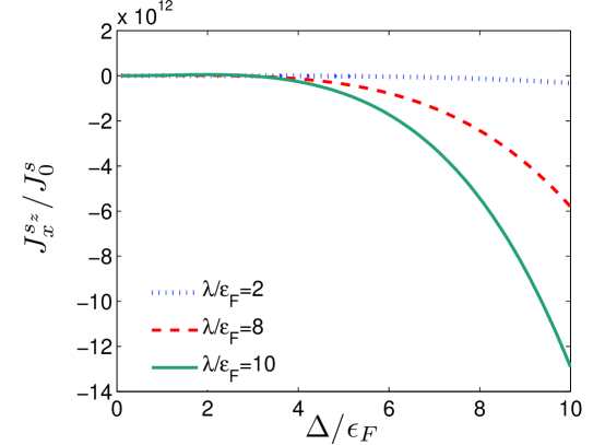
Figure 1: non-equilibrium longitudinal spin current as a function of the graphene gap at different Rashba couplings.

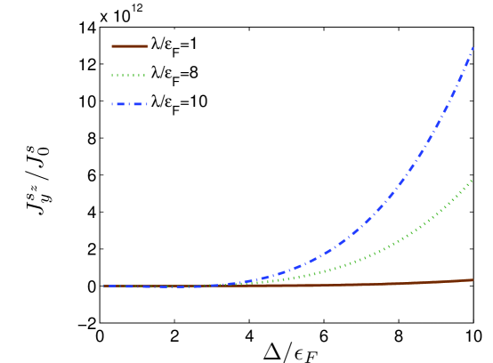
Figure 2: non-equilibrium transverse spin current as a function of the graphene gap at different Rashba couplings.

Figure 3 displays the electric current along the x direction as a function of the gap. As illustrated in this figure the electric current in gaped graphene can be effectively changed by the Rashba coupling. The absolute value of electrical current increases by increasing the amount of the gap. The deference between the curves inside this figure demonstrates the importance of the Rashba coupling.

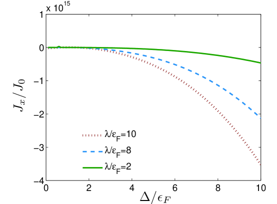
Figure 3: Longitudinal electric current as a function of the gap in graphene at different Rashba couplings.

The longitudinal non-equilibrium spin-currents of a monolayer gapped graphene have indicated as a function of the Rashba coupling in figure 4. The Rashba spin-orbit coupling strength can reach high values up to 0.2eV in monolayer graphene. As shown in this figure, the absolute value of spin-current induced by the Rashba coupling increases by increasing the gap.
As can be seen in figures 1-4, absolute value of spin-current would increase by increasing the Rashba coupling strength and also the energy gap because, on the one hand, the increased energy gap would reduce the possibility of spin relaxation and spin mixing and on the other hand, increased Rashba coupling strength would raise effective magnetic field of this coupling. This effective magnetic field can be regarded as $\textbf{B}_{eff}=\lambda_{R}/(2\mu_{B})(\sigma_{y}\hat{x}-\sigma_{x}\hat{y})$. Anisotropy induced by current-driving electric field results in a non-vanishing average effective magnetic field; i.e. if the current-driving electric field is along with $x$, hopping along with $x$ axis would be more likely to happen and $<\sigma_{x}>~{}>~{}<\sigma_{y}>$ therefore the existing electrons at Fermi level would feel a non-zero effective magnetic field where the spin-current is originating from this field. Therefore, external in-plane electric field plays an important role in generating the effective magnetic field on spin carriers. Consequently, it is expected that, if bias voltage is applied along the $y$ axis, the direction of effective magnetic field would also change; thus, type of spin majority carriers would also modify. This phenomenon can be clearly seen in figures 1-4 so that spin-current sign changes depending on the direction of the applied bias voltage. Therefore, the sign of spin current would be controllable by external bias. According to the mentioned points, generating spin-current of vertical spins at least in non-equilibrium regime can be expected.
The behavior of the spin-current is determined by the impurity density as depicted in figure 5. In this figure, we have taken $\Delta/\epsilon_{F}=5$ and it can be inferred from the data depicted in this figure that increasing the spin-mixing rate (which could take place by increasing the density of impurities) decreases the spin-polarization and spin-current of the system.

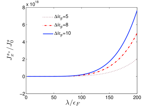
Figure 4: Longitudinal spin current as a function of the Rashba coupling.

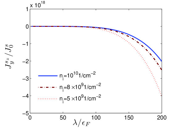
Figure 5: Transverse spin current as a function of the Rashba coupling at $\Delta/\epsilon_{F}=5$.

4 Conclusion

In the present work, the influence of the Rashba coupling on spin-related transport effects have been studied. Results of the present study show that the Rashba interaction has an important role in generation of the non-equilibrium spin-current of vertical spins in a monolayer gapped graphene. The absolute value of spin-current as a function of the gap, increases by increasing the Rashba interaction strength in non-equilibrium regime. Another important point in the results of the present study can be describe as follows; Not only the amount of spin-current in grapheme is controllable by gate voltage (responsible for Rashba interaction) but also its sign is predictable by the direction of the applied bias voltage.

References

References

- [1] Novoselov K S, Geim A K, Morozov S V, Jiang D, Katsnelson M I , Grigorieva I V, Dubonos S V and Firsov A A 2005 Nature 438 197
- [2] Novoselov K S, Geim A K, Morozov S V, Jiang D, Zhang Y, Dubonos S V, Grigorieva I V and Firsov A A 2004 Science 306 666
- [3] Tombros N, Jozsa C, Popinciuc M, Jonkman H T and Wees B J van 2007 Nature 448 571
- [4] Han W, Kawakami R K 2001 Phys. Rev. Lett. 107 047207
- [5] Rashba Emmanuel I 2003 Phys. Rev. B 68 241315
- [6] Rashba E I 1960 Sov. Phys. Solid State 2 1109
- [7] Huertas-Hernando D, Guinea F and Brataas A 2006 Phys. Rev. B 74 155426
- [8] Dedkov Yu S, Fonin M, Rudiger U, and Laubschat C 2008 Phys. Rev. Lett. 100 107602
- [9] Phirouznia A, Shateri S Safari, Poursamad Bonab J, and Jamshidi-Ghaleh K 2012 Applied Physics Letters 101 111905
- [10] Jamshidi-Ghaleh K, Phirouznia A and Sharifnia R 2012 J. Opt. 14 035601
- [11] Soodchomshom B 2011 Physica B 406 614-619
- [12] Ezawa M 2010 Physica E 42 703 706
- [13] Giavaras G and Nori F 2010 Applied Physics Letters 97 243106
- [14] Kane C L and Mele E J 2005 Phys. Rev. Lett 95 226801
- [15] Ahmadi S, Esmaeilzade M, Namvar E and Pan Genhua 2012 AIP ADVANCES 2 012130
- [16] Rashba Emmanuel I 2003 Phys. Rev. B 68 241315
- [17] Yi K S, Kim D and Park K S 2007 Phys. Rev. B 76 115410
- [18] Vitali L, Riedl C, Ohmann R, Brihuega I, Starke U and Kern K, Sci Surf 2008 Lett 127 602
- [19] Zhou S Y, Gweon G-H, Fedorov A V, First P N, de Heer W A, Lee D-H, Guinea F, Castro Neto A H and Lanzara A 2007 Nature Mater 6 770
- [20] Enderlein C, Kim Y S, Bostwick A, Rotenberg E and Horn K 2010 New J. Phys. 12 033014
- [21] Výborný K, Kovalev Alexey A, Sinova J and Jungwirth T 2009 Phys. Rev. B 79 045427
- [22] Huang Zhian and Hu Liangbin 2006 Phys. Rev. B 73 113312
- [23] Inoue Jun-ichiro, Bauer Gerrit E W and Molenkamp Laurens W 2003 Phys. Rev. B 67 033104
- [24] Liewrian W, Hoonsawat R, Tang I-M 2010 Physica E 42 1287-1292