A Combined VLT and Gemini Study of the Atmosphere of the Directly-Imaged Planet, $\beta$ Pictoris b

Abstract

We analyze new/archival VLT/NaCo and Gemini/NICI high-contrast imaging of the young, self-luminous planet $\beta$ Pictoris b in seven near-to-mid IR photometric filters, using advanced image processing methods to achieve high signal-to-noise, high precision measurements. While $\beta$ Pic b’s near-IR colors mimick that of a standard, cloudy early-to-mid L dwarf, it is overluminous in the mid-infrared compared to the field L/T dwarf sequence. Few substellar/planet-mass objects – i.e. $\kappa$ And b and 1RXJ 1609B – match $\beta$ Pic b’s $JHK_{s}L^{\prime}$ photometry, and its 3.1 $\mu m$ and 5 $\mu m$ photometry are particularly difficult to reproduce. Atmosphere models adopting cloud prescriptions and large ($\sim$ 60 $\mu m$) dust grains fail to reproduce the $\beta$ Pic b spectrum. However, models incorporating thick clouds similar to those found for HR 8799 bcde but also with small (a few microns) modal particle sizes yield fits consistent with the data within uncertainties. Assuming solar abundance models, thick clouds, and small dust particles ($<a>$ = 4 $\mu m$) we derive atmosphere parameters of log(g) = 3.8 $\pm$ 0.2 and $T_{eff}$ = 1575–1650 $K$, an inferred mass of 7${}^{+4}_{-3}$ $M_{J}$, and a luminosity of log(L/L_⊙) $\sim$ -3.80 $\pm$ 0.02. The best-estimated planet radius, $\approx$ 1.65 $\pm$ 0.06 $R_{J}$, is near the upper end of allowable planet radii for hot-start models given the host star’s age and likely reflects challenges with constructing accurate atmospheric models. Alternatively, these radii are comfortably consistent with hot-start model predictions if $\beta$ Pic b is younger than $\approx$ 7 Myr, consistent with a late formation, well after its host star’s birth $\sim$ 12${}^{+8}_{-4}$ Myr ago.

1. Introduction

The method of detecting extrasolar planets by direct imaging, even in its current early stage, fills in an important gap in our knowledge of the diversity of planetary systems around nearby stars. Direct imaging searches with the best conventional AO systems (e.g. Keck/NIRC2, VLT/NaCo, Subaru/HiCIAO) are sensitive to very massive planets ($M$ $\gtrsim$ 5–10 $M_{J}$) at wide separation ($a$ $\sim$ 10-30 $AU$ to 100 $AU$) and young ages ($t$ $\lesssim$ 100 Myr), which are not detectable by the radial velocity and transit methods (e.g. Lafrenière et al., 2007a; Vigan et al., 2012; Rameau et al., 2013; Galicher et al., 2013). Planets with these masses and orbital separations pose a stiff challenge to planet formation theories (e.g. Kratter et al., 2010; Rafikov, 2011). Young self-luminous directly-imageable planets provide a critical probe of planet atmospheric evolution (Fortney et al., 2008; Currie et al., 2011a; Spiegel and Burrows, 2012; Konopacky et al., 2013).

The directly-imaged planet around the nearby star $\beta$ Pictoris ($\beta$ Pictoris b) is a particularly clear, crucial test for understanding the formation and atmospheric evolution of gas giant planets (Lagrange et al., 2009a, 2010). At 12${}^{+8}_{-4}$ Myr old (Zuckerman et al., 2001), the $\beta$ Pictoris system provides a way to probe planet atmospheric properties only $\approx$ 5–10 Myr after the disks from which planets form dissipate ($\approx$ 3–10 Myr, e.g. Pascucci et al., 2006; Currie et al., 2009). Similar to the case for the HR 8799 planets (Marois et al., 2010a; Fabrycky and Murray-Clay, 2010; Currie et al., 2011a; Sudol and Haghighipour, 2012), $\beta$ Pic b’s mass can be constrained without depending on highly-uncertain planet cooling models: in this case, RV-derived dynamical mass upper limits when coupled with the range of plausible orbits ($a$ $\sim$ 8–10 AU) imply masses less than $\sim$ 10–15 $M_{J}$ (Lagrange et al., 2012a; Currie et al., 2011b; Chauvin et al., 2012; Bonnefoy et al., 2013), a mass range consistent with estimates derived from the planet’s interaction with the secondary disk (Lagrange et al., 2009a; Dawson et al., 2011).

Furthermore, while other likely/candidate planets such as Fomalhaut b and LkCa 15 b are probably made detectable by circumplanetary emission in some poorly constrained geometery (Currie et al., 2012a; Kraus and Ireland, 2012), $\beta$ Pic b’s emission appears to be consistent with that from a self-luminous planet’s atmosphere (Currie et al., 2011b; Bonnefoy et al., 2013). Other objects of comparable mass appear to have formed more like low-mass binary companions. Thus, combined with the planets HR 8799 bcde, $\beta$ Pic b provides a crucial reference point with which to interpret the properties of many soon-to-be imaged planets with upcoming extreme AO systems like $GPI$, $SCExAO$, and $SPHERE$ (Macintosh et al., 2008; Martinache et al., 2009; Beuzit et al., 2008).

However, investigations into $\beta$ Pic b’s atmosphere are still in an early stage compared to those for the atmospheres of the HR 8799 planets and other very low-mass, young substellar objects (e.g. Currie et al., 2011a; Skemer et al., 2011; Konopacky et al., 2013; Bailey et al., 2013). Of the current published photometry, only $K_{s}$ (2.18 $\mu m$) and $L^{\prime}$ (3.78 $\mu m$) have photometric errors smaller than $\sim$ 0.1 mag (Bonnefoy et al., 2011; Currie et al., 2011b). Other high SNR detections such as at $M^{\prime}$ were obtained without reliable flux calibration (Currie et al., 2011b) or with additional, large photometric uncertainties due to processing (Bonnefoy et al., 2013). As a result, the best-fit models admit a wide range of temperatures, surface gravities, and cloud structures (e.g. Currie et al., 2011b). Thus, new higher signal-to-noise/precision and flux-calibrated photometry at 1–5 $\mu m$ should provide a clearer picture of the clouds, chemistry, temperature, and gravity of $\beta$ Pic b. Moreover, new near-to-mid IR data may identify distinguishing characteristics of $\beta$ Pic b’s atmosphere, much like clouds and non-equilibrium carbon chemistry for HR 8799 bcde (Currie et al., 2011a; Galicher et al., 2011; Skemer et al., 2012; Konopacky et al., 2013).

In this study, we present new 1.5–5 $\mu m$ observations for $\beta$ Pic b obtained with $NaCo$ on the Very Large Telescope and $NICI$ on Gemini-South. We extract the first detection at the 3.09 $\mu m$ water-ice filter; the first high signal-noise, well calibrated H, [4.05], and $M^{\prime}$ detections; and higher signal-to-noise detections at $K_{s}$ and $L^{\prime}$ (2.18 and 3.8 $\mu m$). To our new data, we add rereduced $\beta$ Pic data obtained in $J$ (1.25 $\mu m$) and $H$ (1.65 $\mu m$) bands and first presented in Bonnefoy et al. (2013), recovering $\beta$ Pic b at a slightly higher signal-to-noise and deriving its photometry with smaller errors.

We compare the colors derived from broadband photometry to that for field substellar objects with a range of spectral types to assess whether $\beta$ Pic b’s colors appear anomalous/redder than the field sequence like those for planets around HR 8799 and $\kappa$ And; planet-mass companions like 2M 1207 B, GSC 06214 B, and 1RXJ 1609 B (Chauvin et al., 2004; Ireland et al., 2011; Lafreniére et al., 2008); and other substellar objects like Luhman 16B (Luhman et al., 2013). We use atmosphere modeling to constrain the range of temperatures, surface gravities, and cloud structures plausible for the planet. While previous studies have shown the importance of clouds and non-equilibrium carbon chemistry in fitting the spectra/photometry of directly-imaged planets (Bowler et al., 2010; Currie et al., 2011a; Madhusudhan et al., 2011; Galicher et al., 2011; Skemer et al., 2012; Konopacky et al., 2013), here the assumed sizes of dust particles entrained in the clouds plays a critical role.

2. Observations and Data Reduction

2.1. VLT/NaCo Data and Basic Processing

We observed $\beta$ Pictoris under photometric conditions on 14 December to 17 December 2012 with the NAOS-CONICA instrument (NaCo; Rousset et al., 2003) on the Very Large Telescope UT4/Yepun at Paranal Observatory (Program ID 090.C-0396). All data were taken in pupil-tracking/angular differential imaging (Marois et al., 2006) and data cube mode. Table 1 summarizes the basic properties of these observations. Our full complement of data during the run includes imaging at 1.04 $\mu m$, 2.12 $\mu m$, $K_{s}$/2.18 $\mu m$, 2.32 $\mu m$, 3.74 $\mu m$, $L^{\prime}$/3.78 $\mu m$, Br-$\alpha$/4.05 $\mu m$, and $M^{\prime}$. Here, we focus only on the $L^{\prime}$, [4.05], and $M^{\prime}$ data, deferring the rest to a later study. Each observation was centered on $\beta$ Pictoris’s transit for a total field rotation of $\sim$ 50–70 degrees and a total observing times ranging between $\sim$ 30 minutes and 59 minutes.

To these new observations, we rereduce $J$-band and $H$-band data first presented in Bonnefoy et al. (2013) and taken on 16 December 2011 and 11 January 2012, respectively. The saturated $J$ band science images are bracketed by two sequences of unsaturated images obtained in neutral density filter for flux calibration. While there were additional frames taken but not analyzed in Bonnefoy et al., we found these to be of significantly poorer quality and thus do not consider them here. In total, the $J$-band data we consider covers 40 minutes of integration time and $\sim$ 23^o of field rotation. The $H$-band data cover $\sim$ 92 minutes of integration time and $\sim$ 36^o of field rotation.

Basic NaCo image processing steps were performed as in Currie et al. (2010, 2011b). The thermal IR data at $L^{\prime}$ and [4.05] ($M^{\prime}$) were obtained in a dither pattern with offsets every 2 (1) images to remove the sky background. As all data were obtained in data cube mode, we increased our PSF quality by realigning each individual exposure in the cube to a common center position and clipping out frames with low encircled energy (i.e. those with a core/halo ratio $<$ max(core/halo) - 3$\times$$\sigma$(core-to-halo ratio)).

2.2. Gemini/NICI Data and Basic Processing

We obtained Gemini imaging for $\beta$ Pic b using the Near-Infrared Coronagraphic Imager (NICI) on 23 December 2012 and 26 December 2012 in the H₂O filter ($\lambda_{o}$ = 3.09 $\mu m$) and 9 January 2013 in the $H$ and $K_{s}$ filters (dual-channel imaging), both under photometric conditions (Program GS-2012B-Q-40). These observations were also executed in angular differential imaging mode. For the $H_{2}$$O$ data, we dithered each 38 s exposure for sky subtraction for a total of $\sim$ 38 minutes of integration time over a field rotation of $\sim$ 30 degrees. For the $H/K_{s}$ data, we placed the star behind the $r$ = 0$\farcs$22 partially-transmissive coronagraphic mask to suppress the stellar halo. Here, we took shorter exposures of $\beta$ Pic ($t_{int}$ $\sim$ 11.4 s) to better identify and filter out frames with bad AO correction. Our observing sequence consists of $\sim$ 22 minutes of usable data centered on transit with a field rotation of $\sim$ 41 degrees.

Basic image processing follows steps described above for NaCo data. The PSF halo was saturated out to $r$ $\sim$ 0$\farcs$32–0$\farcs$36 in $H$ during most of the observations and our sequence suffered periodic seeing bubbles that saturated the halo out to angular separations overlapping with the $\beta$ Pic b PSF. Thus, we focus on reducing only those $H$-band frames with less severe halo saturation ($r_{sat}$ $<$ 0$\farcs$36). The $K_{s}$ observations, obtained at a higher Strehl ratio, never suffered halo saturation. The first of the two $H_{2}0$ sets, suffered from severe periodic seeing bubbles and thus generally poor AO performance. We identify and remove from analysis frames whose halo flux exceeded the $F_{min}$+3$\sigma$, where $F_{min}$ is the minimum flux within an aperture covering $\beta$ Pic b and $\sigma$ is the dispersion in this flux: about 10-25% of the frames, depending on the data set in question.

2.3. PSF Subtraction

To remove the noisy stellar halo and reveal $\beta$ Pic b, we process the data with our “adaptive” LOCI (A-LOCI) pipeline (Currie et al., 2012a, b, T. Currie 2013 in prep.). This approach adopts “locally optimized combination of images” (LOCI) formalism (Lafrenière et al., 2007b), where we perform PSF subtraction in small annular regions (the “subtraction zone”) at a time over each image. Previously-described A-LOCI components we use here include “subtraction zone centering” (Currie et al., 2012b); “speckle filtering” to identify and remove images with noise structure poorly correlated with that from the science image we are wanting to subtract (Currie et al., 2012b); a moving pixel mask to increase point source throughput and normalize it as a function of azimuthal angle (Currie et al., 2012a). We do not consider a PSF reference library (Currie et al., 2012a) since $\beta$ Pictoris is our only target.

Into A-LOCI as recently utilized in Currie et al. (2012a), we incorporate a component different from but complementary to our “speckle filtering”, using singular value decomposition (SVD) to limit the number of images used in a given annular region (i.e. for a given optimization zone) to construct and subtract a reference. Briefly, in the (A-)LOCI formalism a matrix inversion yields the set of coefficients $c^{k}$ applied to each image making up the reference “image”: $c^{k}$ = A^-1b. Here, A is the covariance matrix and b is a column matrix defined from $i$ pixels in the “optimization zones” of the $j$-th reference image section O^j and the science image, O^T: b_j = $\sum\limits_{i}$ O${}^{j}_{i}$O${}^{T}_{i}$ (see Lafrenière et al., 2007b). In the previous versions of our codes, we use a simple double-precision matrix inversion to invert the covariance matrix and then solve for $c^{k}$ after multiplying by b.

In this work, we instead use SVD to rewrite A as U$\Sigma$V^T such that A^-1 = V$\Sigma^{-1}$U^T, where the T superscript stands for the transpose of the matrix. Prior to inversion, we truncate the number of singular values at a predefined cutoff, $svd_{lim}$. This eigenvalue truncation is very similar to and functions the same as the truncation of principle components, $N_{pca}$, in the Karhunen-Loeve image projection (KLIP) (Soummer et al., 2012) and has been successfully incorporated before (Marois et al., 2010b). We found that both speckle filtering and SVD truncation within our formalism can yield significant contrast gains over LOCI and KLIP/Principle Component Analysis (PCA), although in this study at the angular separation of $\beta$ Pic b ($\approx$ 0$\farcs$45) the gains over LOCI are typically about a factor of 1.5, albeit with substantially higher throughput.

2.4. Planet Detections

Figures 1, 2, and 3 display reduced NaCo and NICI images of $\beta$ Pic. We detect $\beta$ Pic b in all datasets (summarized in Table 2). To compute the signal-to-noise ratio (SNR) for $\beta$ Pic b, we determine the dispersion, $\sigma$, in pixel values of our final image convolved with a gaussian along a ring with width of 1 FWHM at the same angular separation as $\beta$ Pic b but excluding the planet (e.g. Thalmann et al., 2009), and average the SNR/pixel over the aperture area. For the Gemini-NICI $H$, $K_{s}$, and two [3.1] datasets, the SNRs are thus 6.4, 11, 4.6, and 10, respectively. For the $J$ and $H$-band NaCo data previously presented in Bonnefoy et al. (2013), we achieve SNR $\sim$ 9 and SNR $\sim$ 30, respectively. Generally speaking, our 3.8–5 $\mu m$ NaCo data are deeper than the near-IR NaCo and especially near-IR NICI data, where we detect $\beta$ Pic b at SNR = 40 in $L^{\prime}$ and 22 at $M^{\prime}$, roughly a factor of two higher than previously reported (Currie et al., 2011b; Bonnefoy et al., 2013), gains due to $\beta$ Pic b now being at a wider projected separation ($L^{\prime}$) or post-processing and slightly better observing conditions ($M^{\prime}$). The high SNR detections obtained with NaCo also leverage on recent engineering upgrades that substantially improved the instrument’s image quality and the stability of its PSF (Girard et al., 2012).

The optimal A-LOCI algorithm parameters vary significantly from dataset to dataset. The rotation gap ($\Delta$PA in units of the image full-width half maximum) criterion used to produce most of the images is $\delta$ $\sim$ 0.6–0.65, although it is significantly larger for the $J$ and $H$ data sets ($\delta$ = 0.75–0.95). Generally speaking, the optimization areas we use $N_{A}$ are significantly smaller ($N_{A}$ = 50-150) than those typically adopted (i.e. $N_{A}$=300; Lafrenière et al., 2007b). We speculate that the pixel masking component of A-LOCI drives the optimal $N_{A}$ settings toward these smaller values since the planet flux (ostensibly within the subtraction zone) no longer significantly biases the coefficient determinations to the point of reducing the planet’s SNR. Filtering parameters $r_{corr}$ and $svd_{lim}$ likewise vary wildly from $r_{corr}$ = 0 and $svd_{lim}$ = 2.5$\times$10^-7 at $J$ to $r_{corr}$ = 0.9 for the NICI $H$-band data or $svd_{lim}$ = 2.5$\times$10^-2 for the $M^{\prime}$ NaCo data.

While the many algorithm free parameters make finding an optimal combination difficult and computationally expensive, our final image quality is nevertheless extremely sensitive to some values, in particular $svd_{lim}$ and $r_{corr}$. As a test, we explored other image processing methods – ADI-based classical PSF subtraction and LOCI. While A-LOCI always yields deeper contrasts, we easily detect $\beta$ Pic b in the mid-IR NaCo data using any method and only the poorer of the two [3.1] data sets requires A-LOCI to yield a better than 4-$\sigma$ detection (i.e. where $\sigma_{det}$ = 1.0857/SNR = 0.27 mags). We will present a detailed analysis of image processing methods and algorithm parameters in an upcoming study (T. Currie, 2013 in prep.).

Adopting the pixel scales listed in Table 1, $\beta$ Pic b is detected at an angular separation of $r$ $\sim$ 0$\farcs$46 in each data set. The position angle of $\beta$ Pic b is consistent with previously-listed values (PA $\approx$ 210^o) and in between values for the main disk and the warp, intermediate between the results presented in Currie et al. (2011b) and Lagrange et al. (2012b). While the NICI north position angle on the detector is precisely known and determined from facilty observations, we have not yet used our astrometric standard observations to derive the NaCo position angle offset, which changes every time NaCo is removed from the telescope. To dissuade others from using the poorly calibrated NaCo data and precisely calibrated data (Lagrange et al., 2012b) together, we reserve a detailed determination of $\beta$ Pic b’s astrometry and a study of its orbit for a future study. We also detect the $\beta$ Pic debris disk in each new broadband data set and at [4.05] (Figure 4). We will analyze its properties at a later time as well.

2.5. Planet Photometry

To derive $\beta$ Pic b photometry, we first measured its brightness within an aperture roughly equal to the image FWHM in each case, which was known since we either had AO-corrected standard star observations (NICI $H$, $K_{s}$, and [3.1]), unsaturated images of the primary as seen through the coronagraphic mask (NICI $K_{s}$), unsaturated neutral density filter observations (NaCo $J$, $H$, $L^{\prime}$, and $M^{\prime}$), or unsaturated images of the primary (NaCo $L^{\prime}$ and [4.05]). We assessed and corrected for planet throughput losses due to processing by comparing the flux of synthetic point sources within this aperture implanted into registered images at the same angular separation as $\beta$ Pic b before and after processing. To derive $\beta$ Pic b’s throughput and uncertainty in the throughput ($\sigma_{atten}$), we repeat these measurements at 15 different position angles and adopt the clipped mean of the throughput as our throughput and standard deviation of this mean as its uncertainty. The planet throughput ranges from 0.38 for the $J$-band data to 0.82 for the [4.05] data and 0.96 for the NICI $H$-band data, even with aggressive algorithm parameters (i.e. $\delta$ $\sim$ 0.6), due to the throughput gains yielded by our pixel masking and the SVD cutoff.

For photometric calibration, we followed several different approaches. For the NICI data, we used TYC 7594-1689-1 and HD 38921 as photometric standards. We were only able to obtain photometric calibrations for the first of the two [3.1] datasets. For all other data we used the primary star, $\beta$ Pic, for flux calibration adopting the measurements listed in Bonnefoy et al. (2013). For the $J$ and $H$ NaCo data, we used images of the primary as viewed through the neutral density filter. For the $M^{\prime}$ NaCo data, we obtained neutral density filter observations and very short exposures. While the latter were close to saturation and were probably in the non-linear regime, the implied photometry for $\beta$ Pic was consistent to within errors. The primary was unsaturated in the [4.05]. Finally, for the $L^{\prime}$ data, we took 8.372 ms unsaturated images of $\beta$ Pic for flux calibration. In all cases, we again adopt the clipped mean of individual measurements as our photometric calibration uncertainty, $\sigma_{fluxcal}$. To compute the photometric uncertainty for each data set, we considered the SNR of our detection, the uncertainty in the planet throughput, and the uncertainty in absolute flux calibration: $\sigma$ = $\sqrt{\sigma_{det}^{2}+\sigma_{atten}^{2}+\sigma_{fluxcal}^{2}}$.

Table 2 reports our photometry and Table 3 lists sample error budgets for two NICI photometric measurements and two NaCo measurements. The relative contributions from each source of photometric uncertainty to the total uncertainty are representative of our combined data set. For the [3.09] data, residual speckle noise/sky fluctuations greatly limit the planet’s SNR and thus $\sigma_{det}$ is the primary source of photometric uncertainty. For the $K_{s}$ data, the intrinsic SNR and the two other sources of photometric uncertainty contribute in a more equal proportion. The $L^{\prime}$ and $M^{\prime}$ data error budgets are characteristic of most of our other data, where the photometric uncertainty is primarily due to the absolute photometric calibration and throughput. With the exception of the [3.09] NICI data, the intrinsic SNR of the detection does not dominate the error budget. For the best-quality (mid-IR NaCo) data, the throughput uncertainty was small ($\approx$ 5%) and was never any larger than 15% ($J$ band data) in any data set.

In general, we find fair agreement with previously published photometry, where our measurements are usually consistent within photometric errors with those reported previously (e.g. $m_{H}$= 13.32 $\pm$ 0.14 and 13.25 $\pm$ 0.18 vs. 13.5 $\pm$ 0.2 in Bonnefoy et al. 2013). Our $L^{\prime}$ photometry is more consistent with Currie et al.’s measurement of $m_{L^{\prime}}$=9.73 $\pm$ 0.06 than with that listed in Bonnefoy et al. (2013) ($m_{L^{\prime}}$=9.5 $\pm$ 0.2), though it is nearly identical to that derived for some $\beta$ Pic b data sets listed in Lagrange et al. (2010). Our [4.05] photometry implies that $\beta$ Pic b is $\sim$ 15-20% brighter there than previously assumed (Quanz et al., 2010) and may have a slightly red $L^{\prime}$-[4.05] color. The major difference from previous studies, though, is that our photometric errors are consistently much smaller. For example, the uncertainty in the [4.05] photometry is reduced to 0.08 mag from 0.23 mag due both to higher SNR detections and lower uncertainty in our derived photometry (e.g. throughput corrections). NICI photometry is also substantially less uncertain than in Boccaletti et al. (2013) because $\beta$ Pic b is not occulted by the focal plane mask. These lower uncertainties should allow more robust comparisons between $\beta$ Pic b and other substellar objects and, from modeling, more precise limits on the best-fitting planet atmosphere properties.

3. Empirical Comparisons to $\beta$ Pic b

Our new data allows us to compare the spectral energy distribution of $\beta$ Pic b to that for the many field L/T-type brown dwarfs as well that for directly-imaged low-surface gravity, low-mass brown dwarf companions and directly-imaged planets. Our goal here is to place $\beta$ Pic b within the general L/T type spectral sequence, identify departures from this sequence such as those seen for low surface gravity objects like HR 8799 bcde, and identify the substellar object(s) with the best-matched SED. Some bona fide directly-imaged planets like HR 8799 bcde and at least some of the lowest-mass brown dwarfs like 2M 1207 B appear redder/cloudier than their field dwarf counterparts at comparable temperatures ($T_{eff}$ $\approx$ 900-1100 $K$). However, it is unclear whether hotter imaged exoplanets appear different from their (already cloudy) field L dwarf counterparts, and $\beta$ Pic b provides a test of any such differences. We will use our comparisons to the L/T dwarf sequence and the SEDs of other substellar objects to inform our atmosphere model comparisons later to derive planet physical parameters (e.g. $T_{eff}$ and log(g)).

3.1. Infrared Colors of $\beta$ Pic b

To compare the near-to-mid IR properties of $\beta$ Pic b with those for other cool, substellar objects, we primarily use the sample of L/T dwarfs compiled by Leggett et al. (2010), which include field dwarfs spectral classes between $\sim$ M7 and T5, corresponding to a range of temperatures between $\sim$ 2500 $K$ and 700 $K$. To explore how the $\beta$ Pic b SED compares to those with other directly-imaged planets/planet candidates and very low-mass brown dwarf companions within this temperature range, we include objects listed in Table 4. These include the directly-imaged planets around HR 8799 (Marois et al., 2008, 2010a; Currie et al., 2011a) and the directly-imaged planet candidate around $\kappa$ And (Carson et al., 2013). Additionally, we include high mass ratio brown dwarf companions with masses less than the deuterium-burning limit ($\sim$ 13–14 $M_{J}$) and higher-mass companions whose youth likely favors a lower surface gravity than for field brown dwarfs, a difference that affect the objects’ spectra (e.g. Luhman et al., 2007). Among these objects are 1RXJ 1609B, AB Pic B, and Luhman 16 B (Lafreniére et al., 2008; Chauvin et al., 2005; Luhman et al., 2013). Table 5 compiles photometry for all of these low surface gravity objects.

Figure 5 compares the IR colors of $\beta$ Pic b (dark blue diamonds) to those for field M dwarfs (small black dots), field L0–L5 dwarfs (grey dots), field L5.1-L9 dwarfs (asterisks), T dwarfs (small light-grey dots), and planets/low-mass young brown dwarfs (light-blue squares). The $J$-$H$/$H$-$K_{s}$ colors for $\beta$ Pic b appear slightly blue in $J$-$H$ and red in $H$-$K_{s}$ compared to field L0–L5 dwarfs, though the difference here is not as large as was found in Bonnefoy et al. (2013). Other young substellar objects appear to have similar near-IR colors, in particular $\kappa$ And b, GSC 06214 B, USco CTIO 108B, 2M 1207A, and Luhman 16 B, whose spectral types range between M8 and T0.5.

The mid-IR colors of $\beta$ Pic b (top-right and bottom panels) show a more complicated situation. In $J$-$K_{s}$/$K_{s}$-$L^{\prime}$ and $H$-$K_{s}$/$K_{s}$-$L^{\prime}$, $\beta$ Pic b lies along the field L/T dwarf locus with colors in between those for L0–L5 and L5.1–L9 dwarfs, overlapping in color with $\kappa$ And b, 1RXJ 1609B, GSC 06214B, HR 8799 d, and 2M 1207 B. Compared to the few field L/T dwarfs from the Leggett et al. sample with $M^{\prime}$ photometry, $\beta$ Pic b appears rather red, most similar in $K_{s}$-$M^{\prime}$ color to GSC 06214 B.

The color-magnitude diagram positions of $\beta$ Pic b (Figure 6) better clarify how its near-to-mid SED compares to the field L/T dwarf sequence and to very low-mass (and gravity?) young substellar objects. In general, compared to the field L dwarf sequence, $\beta$ Pic b appears progressively redder at mid-IR wavelengths. Similar to the case for GSC 06214 B (Bailey et al., 2013), $\beta$ Pic b appears overluminous compared to the entire L/T dwarf sequence in the mid-IR.

3.2. Comparisons to SEDs of Other Substellar Objects

To further explore how the SED of $\beta$ Pic b agrees with/departs from the field L/T dwarf sequence and other young substellar objects, we first compare its photometry to spectra from the SPeX library (Cushing et al., 2005; Rayner et al., 2009) of brown dwarfs with data overlapping with our narrowband mid-IR filters ([3.09] and [4.05]) spanning spectral classes between L1 and L5: 2MASS J14392836+1929149 (L1), Kelu-1AB (L2), 2MASS J15065441+1321060 (L3), 2MASS J15074769-1627386 (L5). To compare the $\beta$ Pic b photometry with cooler L dwarfs, we add combined IRTF/SpeX and Subaru/IRCS spectra from 1 to 4.1 $\mu m$ for 2MASS J08251968+2115521 (L7.5) and DENIS-P J025503.3-470049 (L8) (Cushing et al., 2008). Finally, we add spectra for the low surface-gravity L4.5 dwarf, 2MASSJ22244381-0158521 (Cushing et al., 2008). To highlight differences between $\beta$ Pic b and these L dwarfs, we scale the flux densities for each of these standards to match $\beta$ Pic b at $\sim$ 2.15 $\mu m$ ($K_{s}$ band).

To convert our photometry derived in magnitudes to flux density units, we use the zeropoint fluxes listed in Table 6. The $JHK_{s}$ and $L^{\prime}$$M^{\prime}$(4.78 $\mu m$) zeropoints are from Cohen et al. (2003) and Tokunaga and Vacca (2005), respectively. We base the other zeropoints off of Rieke et al. (2008), although alternate sources (e.g. Cohen et al., 1995) yield nearly identical values. Because the overlap in wavelengths between $\beta$ Pic and these objects is not uniform, we do not perform a rigorous fit between the two, finding the scaling factor that minimizes the $\chi^{2}$ value defined from the planet flux density, comparison object flux density, and photometric errors in both. Rather, we focus on a simple first-order comparison between $\beta$ Pic b and the comparison objects to motivate detailed atmospheric modeling later in Section 4.

Figure 7 (left panel) compares photometry for $\beta$ Pic b to spectra for field L1–L5 dwarfs. While the L1 standard slightly overpredicts the flux density at $J$ band, the other three early/mid L standards match the $\beta$ Pic b near-IR SED quite well, indicating a “near-IR spectral type” of $\sim$ L2–L5. The L7.5 and L8 standards also produce reasonable matches, although they tend to underpredict the brightness at $J$ band (right panel).

However, all standards have difficulty matching the $\beta$ Pic b SED from 3–4 $\mu m$. In particular, the $\beta$ Pic b flux density from $\sim$ 3 to $\sim$ 5 $\mu m$ is nearly constant, whereas it rises through 4 $\mu m$ and then steeply drops in all six standards depicted here. Focused on only $\beta$ Pic b photometry at 3.8–4.1 $\mu m$, the “mid-IR spectral type” is hard to define, the low surface gravity L4.5 dwarf bears the greatest resemblance, although we fail to identify good matches at all wavelengths with any of our spectral templates, where the 3.1 $\mu m$, $L^{\prime}$, and [4.05] data points are the most problematic. While none of our standards have measurements fully overlapping with the $M^{\prime}$ filter, the flux densities at 5.1 $\mu m$ indicate that they may have a very hard time simultaneously reproducing our measurements at all four filters between 3 and 5 $\mu m$. Although non-equilibrium carbon chemistry can flatten the spectra of low surface gravity L/T dwarfs (Skemer et al., 2012), its effect is to weaken the methane absorption trough at $\sim$ 3.3 $\mu m$ and suppress emission at $\sim$ 5 $\mu m$. Thus, it is unclear whether this effect can explain the enhanced emission at $\sim$ 3.1 $\mu m$ (mostly outside of the $CH_{4}$ absorption feature to begin with) and 5 $\mu m$.

To understand whether $\beta$ Pic b’s SED is unique even amongst other very low-mass substellar objects, we compare our photometry to that for companions listed in Table 4 that have photometry from 1 $\mu m$ through $\sim$ 4–5 $\mu m$: HR 8799 bcd, $\kappa$ And b, 1RXJ 1609 B, GSC 06214B, HIP 78530 B, 2M 1207A/B, HR 7329B, and AB Pic. Two objects – 1RXJ 1609 B and GSC 06214B – have 3.1 $\mu m$ photometry: 1RXJ 1609 B from (Bailey et al., 2013) and $\kappa$ And b has [4.05] from data obtained by T. C. (M_[4.05] = 9.45 $\pm$ 0.20) (Bonnefoy, Currie et al., 2013 in prep.).

The two far-right columns of Table 5 lists the reduced $\chi^{2}$ and goodness-of-fit statistics between $\beta$ Pic b’s $JHK_{s}L^{\prime}$ ([3.1],[4.05]) photometry, while Figure 8 displays these comparisons for $\kappa$ And b, 1RXJ 1609B, and GSC 06214B, which are all thought to be low surface gravity companions with $T_{eff}$ $\sim$ 1700 K, 1800 K, and 2200 K (Carson et al., 2013; Lafrenière et al., 2010; Bowler et al., 2011; Bailey et al., 2013). Overall, $\kappa$ And b provides the best match to $\beta$ Pic b’s photometry, requires negligible flux scaling, and is essentially the same within the 68% confidence limit (C.L.) ($\chi^{2}$ = 0.946, C.L. = 0.186), although the large photometric uncertainties in the near-IR limit the robustness of these conclusions. The companion to 1RXJ 1609 likewise produces a very good match ($\chi^{2}$ = 1.369, C.L. = 0.287), while the slightly more luminous (and massive) GSC 06214B appears to be much bluer, (relatively) overluminous in $L^{\prime}$ and $M^{\prime}$ (or, conversely, overluminous at $JHK_{s}$) by $\sim$ 30%. In comparison, the cooler ($T_{eff}$ $\approx$ 900-1100 $K$) exoplanets HR 8799 bcd provide far poorer matches ($\chi^{2}$ $\sim$ 6–52).

Still, it is unclear whether any object matches $\beta$ Pic b’s photometry at all wavelengths: both of the objects for which we have [3.1] data, GSC 06214B and 1RXJ 1609B, are still slightly underluminous here. Moreover, the best-matching companions – $\kappa$ And b and 1RXJ 1609B – are still not identical, as the scaling factors between $\beta$ Pic b’s spectrum and these companions’ spectra that minimize $\chi^{2}$ are $\sim$ 0.83 and 0.53, respectively. While companions with identical temperatures but radii 10% and 30% larger than $\beta$ Pic b would achieve this scaling, $\kappa$ And b and 1RXJ 1609B are respectively older and younger than $\beta$ Pic b, whereas for a given initial entropy of formation planet radii are expected to decrease with time (Spiegel and Burrows, 2012).

In summary, young (low surface gravity?), low-mass objects may provide a better match to $\beta$ Pic b’s photometry than do field dwarfs, especially those with temperatures well above 1000 $K$ but slightly below 2000 $K$ ($\kappa$ And b, 1RXJ 1609 B). However, we fail to find a match (within error bars) between the planet’s photometry spanning the full range of wavelengths for which we have data, especially at $\sim$ 3 $\mu m$. As the planet spectra depend critically on temperature, surface gravity, clouds and (as we shall see) dust particle sizes, our comparisons imply that $\beta$ Pic b may differ from most young substellar objects in one of these respects. Next, we turn to detailed atmospheric modeling to identify the set of atmospheric parameters that best fit the $\beta$ Pic b data.

4. Planet Atmosphere Modeling

To further explore the physical properties of $\beta$ Pic b, we compare its photometry to planet atmosphere models adopting a range of surface gravities, effective temperatures, and cloud prescriptions/dust. For a given surface gravity and effective temperature, a planet’s emitted spectrum depends primarily on the atmosphere’s composition, the structure of its clouds, and the sizes of the dust particles of which the clouds are comprised (Burrows et al., 2006). For simplicity, we assume solar abundances except where noted and leave consideration of anomalous abundances for future work.

Based on $\beta$ Pic b’s expected luminosity (log(L${}_{p}/L_{\odot}$) $\sim$ -3.7 to -4, Lagrange et al. 2010; Bonnefoy et al. 2013) and age, it is likely too hot ($T_{eff}$ $\sim$ 1400-1800 K) for non-equilibrium carbon chemistry to play a dominant role (Hubeny and Burrows, 2007; Galicher et al., 2011). Therefore, our atmosphere models primarily differ in their treatment of clouds and the dust particles entrained in clouds. For each model, we explore a range of surface gravities and effective temperatures.

4.1. Limiting Cases: The Burrows et al. (2006) E60 and A60 Models and AMES-DUSTY Models

4.1.1 Model Descriptions

We begin by applying an illustrative collection of previously-developed atmosphere models to $\beta$ Pic b. These models will produce limiting cases for the planet’s cloud structure and typical dust grain size, which we refine in Section 4.2. To probe the impact of cloud thickness, we first adopt a (large) modal particle size of 60 $\mu$m and consider three different cloud models: the standard chemical equilibrium atmosphere thin-cloud models from Burrows et al. (2006), which successfully reproduces the spectra of field L dwarfs, moderately-thick cloud models from Madhusudhan et al. (2011), and thick cloud models used in Currie et al. (2011a). To investigate the impact of particle size, we then apply the AMES-DUSTY models. The DUSTY models lack any dust grain sedimentation, such that the dust grains are everywhere in the atmosphere, similar to the distribution of dust grains entrained in thick clouds. However, they adopt far smaller dust grains than do the thick cloud models from Madhusudhan et al. (2011) and Currie et al. (2011a), where the grains are submicron in size and follow the interstellar grain size distribution (Allard et al., 2001). All models described here and elsewhere in the paper assume that the planet is in hydrostatic and radiative equilibrium. None of them consider irradiation from the star, as this is likely unimportant at $\beta$ Pic b’s orbital separation. Table 7 summarizes the range of atmospheric properties we consider for each model.

The Burrows et al. (2006) E60 Thin Cloud, Large Dust Particle Models – As described in Burrows et al. (2006) and later works (e.g. Currie et al., 2011a; Madhusudhan et al., 2011), the Model E60 case assumes that the clouds are confined to a thin layer, where the thickness of the flat part of the cloud encompasses the condensation points of different species with different temperature-pressure point intercepts. Above and below this flat portion, the cloud shape function decays as the -6 and -10 powers respectively, so that the clouds have scale heights of $\sim$ 1/7th and 1/11th that of the gas. We adopt a modal particle size of 60 $\mu m$ and a particle size distribution drawn from terrestrial water clouds (Deirmendjian, 1964). We consider surface gravities with log(g) = 4 and 4.5 and temperatures with a range of $T_{eff}$ = 1400–1800 K in increments of 100 K.

The Madhusudhan et al. (2011) AE60 Moderately-Thick Cloud, Large Dust Particle Models – Described in Madhusudhan et al. (2011), the Model AE60 case assumes a shallower cloud shape function of $s_{u}$ = 1, such that the cloud scale height is half that of the gas as a whole. We again adopt a modal particle size of 60 $\mu m$ and the same particle size distribution. We consider surface gravities with log(g) = 4 and 4.5 and temperatures between $T_{eff}$ = 1000–1700 K in increments of 100 K.

The Burrows et al. (2006) A60 Thick Cloud, Large Dust Particle Models – As described in Currie et al. (2011a), the Model A60 case differs in that it assumes that the clouds extend with a scale height that tracks that of the gas as a whole. Below the flat part of the cloud, the shape function decays as the -10 power as in the E60 and AE60 models, although deviations from this do not affect the emergent spectrum. Here, we consider surface gravities with log(g) = 4 and 4.5 and temperatures with a range of $T_{eff}$ = 1000-1700 K in increments of 100 K.

AMES-DUSTY Thick-Cloud, Small Dust Particle Limit – The AMES-DUSTY atmosphere models (Allard et al., 2001) leverage on the PHOENIX radiative transfer code (Hauschildt and Baron, 1999) and explore the limiting case where dust grains do not sediment/rain out in the atmosphere. Unlike the Burrows et al. (2006) models and those considered in later works (e.g. Spiegel and Burrows, 2012), the AMES-DUSTY models adopt a interstellar grain size distribution favoring far tinier dust grains with higher opacities. The grains’ higher opacities reduce the planet’s radiation at shorter wavelengths. Thus, these models have dramatically different near-IR planet spectra from the E/A/AE60 type models with larger modal grain sizes even at the same temperatures and gravities (cf. Burrows et al., 2006; Currie et al., 2011a). Here we consider AMES-DUSTY models with log(g) = 3.5, 4, and 4.5 and $T_{eff}$ = 1000–2000 K ($\Delta T_{eff}$=100 K).

4.1.2 Fitting Method

To transform the DUSTY spectra into predicted flux density measurements (at 10 $pc$), we convolve the spectra over the filter response functions and scale by a dilution factor of f = ($R_{planet}$/10 pc)². We consider a range of planet radii between 0.9 $R_{J}$ and 2 $R_{J}$. Likewise, we convolve the E60 and A60 model spectra over filter response functions. The E60 models (as do all other Burrows et al. 2006 and Madhusudhan et al. 2011 models) adopt a mapping between planet radius and surface gravity/temperature set by the Burrows et al. (1997) planet evolution models. To explore departures from these models, we allow the the radius to vary by an additional scale factor of 0.7 to 1.7. For most of our grid, this translates into a radius range of 0.9 to 2 $R_{J}$.

Our atmosphere model fitting follows methods in Currie et al. (2011a, b), where we quantify the model fits with the $\chi^{2}$ statistic,

$$\chi^{2}=\sum\limits_{i=0}^{n}(f_{data,i}-F_{model,i})^{2}/\sigma_{data,i}^{2}.$$ (1)

We weight each datapoint equally. Because our photometric calibration fully considers uncertainties due to the signal-to-noise ratio, the processing-induced attentuation, and the absolute photometric calibration, we do not set a 0.1 mag floor to $\sigma$ for each data point as we have done previously.

We determine which models are formally consistent with the data by comparing the resulting $\chi^{2}$ value to that identifying the 68% and identify those that can clearly be ruled out by computed the 95% confidence limit. Note here that these limits are significantly more stringent compared to the ones we adopted in Currie et al. (2011a). Treating the planet radius as a free parameter, we have five degrees of freedom for seven data points, leading to $\chi^{2}_{68\%}$ = 5.87 and $\chi^{2}_{95\%}$ = 11.06. ‘

4.1.3 Results

Table 8 summarizes our fitting results using the E60, AE60, A60, and DUSTY models. Figure 9 displays some of these fitting results, where the left-hand panels show the $\chi^{2}$ distributions with the 68% and 95% confidence limits indicated by horizontal lines dashed and dotted lines. The right-hand panels and middle-left panel show the best-fitting models for each atmosphere prescription. A successful model must match three key properties of the observed SED: (1) At 3–5 $\mu$m, the SED is relatively flat, (2) at 1–3 $\mu$m, the spectral slope is relatively shallow, and (3) the overall normalization of the 3–5 $\mu$m flux relative to the 1–3 $\mu$m flux must match the data.

For the E60, AE60, and A60 models, we find $\chi^{2}$ minima at log(g) = 4–4.5 and $T_{eff}$ = 1400 $K$ in each case with radius scaling factors, the constant we multiple the nominal Burrows et al. planet radii, between 1.185 and 1.680. For the Burrows et al. (1997) evolutionary models, these scaling factors imply planet radii between $\sim$ 1.8 and 2 $R_{J}$, at the upper extrema of our grid in radius.

Figure 9 illustrates the impact on the SED of changing cloud models, given a fixed grain size. The best-fit temperature does not vary dramatically because, roughly speaking, the relative fluxes at 1–3 $\mu$m and 3–5$\mu$m are determined by the SED’s blackbody envelope. However, cloud thickness dramatically affects the depths of absorption bands superimposed on that envelope. Atmosphere models presented here do not feature temperature inversions. As such, high opacity molecular lines have low flux densities because they originate at high altitudes where the temperature is low. When clouds are thin, optical depth unity is achieved at very different altitudes in and outside of absorption bands such as those at 3.3$\mu$m (methane) and 4.5 $\mu$m (primarily CO), and the bands appear deep.

For a fixed observed effective temperature, thicker clouds translate into hotter temperature profiles (i.e. at a given pressure in the atmosphere, the temperature is higher) (e.g. Madhusudhan et al., 2011). The total Rosseland mean optical depth of the atmosphere at a given pressure is higher (Madhusudhan et al., 2011). As the clouds become thicker, the $\tau$ = 1 surface also is more uniform, such that molecular features wash out and the spectrum overall appears flatter and more like a blackbody (Burrows et al., 2006). Hence, the prominent molecular absorption bands seen in the best-fit E60 (thin cloud) model are substantially reduced in the A60 (thick cloud) model, with AE60 lying in between. The planet’s flat 3–5 $\mu$m SED is best fit by A60.

Although the $\chi^{2}$ minima for all four of the models we consider are sharply peaked, none yield fits falling within the 68% confidence interval. The fits from E60 and AE60 are particularly poor, ruled out at a greater than 5-$\sigma$ level, whereas the A60 model quantitatively does better but still is ruled out as an acceptably-fitting model (C.L. $\sim$ 3.9-$\sigma$). The best-fit AMES-DUSTY model fits the SED even better than A60, with parameters of $T_{eff}$ = 1700 and log(g) = 3.5 and a radius of $r$ = 1.35 $R_{J}$, similar parameters to those found in Bonnefoy et al. (2013). However, the best-fit DUSTY model still falls outside the 68% confidence limit (C.L. = 0.84). These exercises suggest that the atmospheric parameters assumed in the models need to be modified in order to better reproduce the $\beta$ Pic b photometry. To achieve this, we restrict ourselves to thick clouds and consider more carefully the impact of dust size.

4.2. A4, Thick Cloud/Small Dust Models

4.2.1 The Effect of Small Dust Particles

Our analyses in the previous section show the extreme mismatch between standard L dwarf atmosphere models assuming thin clouds and large dust particles and the data. While our $\chi^{2}$ values for the Burrows thick cloud, large dust particle models are systematically much lower, they likewise are a poor match to the data. In contrast, fits from the AMES-DUSTY models only narrowly lie outside the 68% confidence interval.

A closer inspection of the best-fitting models in each case (right-hand panels) illustrates how they fail. The main difficulty with matching these models to $\beta$ Pic b spectrum is the planet’s flat SED from 2 $\mu m$ to 5 $\mu m$, where models tend to underpredict the flux density at 3.1 $\mu m$ and/or $M^{\prime}$. The slope from $J$ to $K_{s}$ is also a challenge. Reducing dust sizes can further fill in absorption troughs by increasing the opacities of the clouds. The AMES-DUSTY model, however, appears to overcorrect as its spectrum exhibits sharp peaks due to its submicron sized grains that degrade its fit to the data. Therefore, we consider grain sizes intermediate between those in A60 and AMES-DUSTY (e.g. $\sim$ 1–30 $\mu m$).

A4 Thick Cloud, Small Dust Particle Models – As the primary difference between these models is the typical/modal particle size, we here introduce a new set of atmosphere models with the same A-type, thick cloud assumption but with modal particle sizes slightly larger than those characteristic of dust in the AMES-DUSTY models but significantly smaller than previous Burrows models. We nominally adopt 4 $\mu m$ as our new modal particle size, comparable in wavelength to the peak flux density of $\beta$ Pic b in $F_{\nu}$ units. Thus, we denote these models as “A4”, thick-cloud, small dust particle models.

Figure 10 illustrates the effect of dust on the planet spectrum for modal particle sizes of 3, 5, 30 and 50 $\mu m$ and a temperature and surface gravity consistent with that expected to reflect $\beta$ Pic b based on planet cooling models ($T_{eff}$ = 1600 K, log(g)=3.8-4, $r$ $\sim$ 1.5 $R_{J}$) (Burrows et al., 1997; Baraffe et al., 2003; Lagrange et al., 2010; Spiegel and Burrows, 2012; Bonnefoy et al., 2013). As particle sizes decrease, the water absorption troughs at 1.8 $\mu m$ and 2.5 $\mu m$ diminish. Likewise filled in is the deep absorption trough at $\sim$ 3.3 $\mu m$ and 4.5 $\mu m$ that is usually diagnostic of carbon chemistry (e.g. Hubeny and Burrows, 2007; Galicher et al., 2011). Overall, the spectrum flattens and becomes redder (shorter wavelength emission originates at higher altitudes), with weaker emission and a steeper slope at $J$ to $K_{s}$. This reddening explains the difference in best-fit effective temperature between the AMES-DUSTY model and the 60 $\mu$m dust models.

4.2.2 Model Fitting Procedure

We follow the steps outlined in Currie et al. (2011a), where we perform two runs: one fixing the planet radius to the Burrows et al. (1997) hot-start predictions for a given $T_{eff}$ and log(g) and another where we consider a range of planet radii (as in the previous section). For the fixed-radii modeling, the 68% and 95% confidence limits now lie at $\chi^{2}$ = 7.01 and 12.6, respectively, whereas they are at 5.87 and 11.06 for the varying-radii fits as before. Similar to the Burrows A/E60 model runs, we consider a range of temperatures between 1400 K and 1900 K. To explore whether or not the fits are sensitive to surface gravity, we consider models with log(g) = 3.6, 3.8, 4, and log(g) = 4.25. For the age of $\beta$ Pic (formally, 8 to 20 Myr), this surface gravity range fully explores the masses (in the hot-start formalism) allowed given the radial-velocity dynamical mass limits (Lagrange et al., 2012a).

To further explore the effect that carbon chemistry may have on our planet spectra, we take the best-fitting model from the above exercise, significantly enhance the methane abundances over solar and re-run a small grid of temperatures based on that, to determine if departures from solar abundances may yield a wider range of acceptable atmosphere parameters. Because variations in molecular abundances affect the depths of molecular absorption bands, we expect that such variations may improve our fit.

4.2.3 Results

Figures 11 and 12 and Table 8 present our results for fitting the $\beta$ Pic b data with the A4, thick cloud/small dust models. Quantitatively, these models better reproduce the $\beta$ Pic b SED. Fixing the planet radius to values assumed in the Burrows et al. (1997) planet cooling model, we find one atmosphere model – log(g) = 3.8, $T_{eff}$ = 1600 $K$ – consistent with the data to within the 68% confidence interval. A wide range of models are consistent with the data at the 95% confidence limit, covering $\pm$ 0.2 dex in surface gravity and $\pm$ 100 $K$ in temperature.

We can slightly improve upon these fits if we allow the planet radius to freely vary. In this case, the best-fitting models yield a slightly higher surface gravity of log(g) = 4–4.25 but the same temperature of 1600 $K$. But in contrast to the fixed-radius case above, a wide range of models are consistent with the data at the 68% confidence limit. In particular, all surface gravities considered in our model grid are consistent with the data provided that the temperature is 1600 $K$ and the radius is rescaled accordingly: log(g) = 3.6–4.25, $T_{eff}$ = 1600 $K$. Another set of models with the full range of surface gravities and 250 $K$ spread in temperature (1500–1750 $K$) are marginally consistent with the data.

The methane-enhanced models are shown in Figure 13 for log(g)=4 and $T_{eff}$ = 1575–1650 $K$. The 1575 $K$ and 1600 $K$ models (Figure 13) likewise produce good fits to the data ($\chi^{2}$ = 5.13–5.3), where the 1650 $K$ model barely misses the 68% cutoff. Thus, while best-fitting solar abundance models appear narrowly peaked at $T_{eff}$ = 1600 $K$, the range in temperature enclosing the 68% confidence interval is larger when non-solar abundances are considered, at least extending from 1575 $K$ to almost 1650 $K$. Changes in molecular abundances, as expected, allow us to very slightly improve the SED fit. However, thick clouds and small dust grains are likely still needed to match the emission from $\beta$ Pic b, since given molecules (i.e. $CH_{4}$) by themselves do not change fluxes comparably at 1–3 $\mu$m and 3–5 $\mu$m.

In summary, adopting the Burrows et al. (1997) hot-start models to set our planet radii and the A4 thick cloud/small dust atmosphere models, we derive log(g) = 3.8 and $T_{eff}$ = 1600 $K$ for $\beta$ Pic b. Allowing the radius to vary and considering non-solar carbon abundances we derive log(g) = 3.6–4.25 and $T_{eff}$ = 1575–1650 $K$, meaning that the planet temperature is well constrained but the surface gravity is not. However, in Section 5 we narrow the range of surface gravities to log(g) = 3.8 $\pm$ 0.2, as higher surface gravities imply planet masses ruled out by dynamical estimates.

4.2.4 Varying Grain Sizes and Fits Over Other Model Parameter Space

The models considered in the previous subsections assume thick clouds, dust grains with a modal size of 4 $\mu m$, and (in most cases) solar abundances. Although we achieve statistically significant fits to the $\beta$ Pic b photometry with these models, our exploration of model parameter space is still limited. While an exhaustive parameter space search is beyond the scope of this paper, here we argue that models either thick clouds or small dust grains are unlikely to produce good-fitting models. Thus, small grains and thick clouds are likely important components of $\beta$ Pic b’s atmosphere required in order to fit the planet’s spectrum.

To consider the robustness of our results concerning the modal grain size, we also ran some model fits for modal particle sizes of 3 $\mu m$, 5 $\mu m$, 10 $\mu m$, and 30 $\mu m$. The models with 3 and 5 $\mu m$ modal sizes yielded fits slightly worse than those with modal sizes of 4 $\mu m$. For example, models with modal sizes of $<a>$ = 3 and 5 $\mu m$, $T_{eff}$ = 1600 K, log(g) = 3.8 and a freely-varying planet radius yield $\chi^{2}$ 6.31 and 6.28, respectively. These values lie slightly outside the 68% confidence interval, although they are still smaller than those from the best-fit DUSTY models. In contrast, models with $<a>$ = 10 $\mu m$ and 30 $\mu m$ fit the data significantly worse ($\chi^{2}$ = 10.0 and 19.6, respectively).

Similarly, our investigations show that small dust grains do not obviate the need to assume thick, A-type clouds in our atmosphere models. For example, adopting the AE-type cloud prescription, modal particle sizes of 5 $\mu m$, a temperature of $T_{eff}$ = 1600 K, and a surface gravity of log(g) = 3.8–4, our model fits are substantiailly worse than the A4-type models and even the AMES-DUSTY models and are easily ruled out ($\chi^{2}$ $\sim$ 15–40). The AE-type cloud prescription fails to reproduce the $\beta$ Pic b spectrum because by confining clouds to a thinner layer the $\tau$ = 1 surface varies too much in and out of molecular absorption features such as $CH_{4}$ and $CO$. In disagreement with the $\beta$ Pic b SED, the AE model spectra thus have suppressed emission at $\approx$ 3 $\mu m$ and 5 $\mu m$ and an overall shape looking less like a blackbody.

In contrast, non-solar abundances may slightly widen the range of parameter space (in radius, temperature, gravity, etc.) yielding good fits. The methane-rich model from the previous section adopting $<a>$ = 5 $\mu m$ instead of 4 $\mu m$, log(g) = 3.8, and $T_{eff}$ = 1600 K still yields a fit in agreement with the data to within the 68% confidence limit ($\chi^{2}$ = 5.59). Thus, within our atmosphere modeling approach we need 1) grains several microns in size, comparable to the typical sizes of grains in debris disks, and 2) thick clouds to yield fits consistent with the data to within the 68% confidence limit. These results are not strongly sensitive to chemical abundances although varying the range of abundances may slightly widen the corresponding range of other parameter space (in temperature, gravity, etc.) yielding good-fitting models.

5. Planet Radii, Luminosities, Masses, and Evolution

From the set of models that reproduce the $\beta$ Pic b SED to the 68% confidence interval, we derive a range of planet radii, luminosities and inferred masses. The planet radii for each model run are given in Table 8. Interestingly, all of our 1-$\sigma$ solutions fall on or about $R$ $\sim$ 1.65 $R_{J}$ with very little dispersion ($\pm$ $\sim$ 0.05 dex). If we consider the range of radii for a given atmosphere model consistent with the data to within the 68% (or 95%) confidence interval regardless of whether the given radius is the best-fit one, then the range in acceptable radii marginally broadens: $r$ = 1.65 $\pm$ 0.06. Note that these radii are larger than those inferred for HR 8799 bcde based either on its luminosity and hot-start cooling tracks (Marois et al., 2008, 2010a) or from atmosphere modeling, where in Currie et al. (2011a) and Madhusudhan et al. (2011) our best-fit models typically had $R$ $\sim$ 1.3 $R_{J}$. The range in inferred planet luminosities is even narrower, The values inferred from our best-fit models center on log($L$/$L_{\odot}$)= -3.80 with negligible intrinsic dispersion ($\pm$ 0.01 dex). The uncertainty in $\beta$ Pic’s distance affects both our radius and luminosity determinations. Treating the distance uncertainty ($\pm$ 1 $pc$) as a separate, additive source of error, $\beta$ Pic b’s range in radii is 1.65 $\pm$ 0.06 $R_{J}$ and its luminosity is log($L$/$L_{\odot}$)= -3.80 $\pm$ 0.02.

From our best-fit surface gravities and inferred radii, we can derive the mass of the planets inferred from our modeling. Adopting the hot-start formalism without rescaling the radius, our modeling implies a best-fit planet mass of $\sim$ 7 $M_{J}$; the range covering the 95% confidence limit of 5–9 $M_{J}$. If we allow the radius to freely vary, we derive a range of 4 $M_{J}$ to 18.7 $M_{J}$, where the spread in mass reflects primarily the spread in surface gravity from best-fitting models (log(g) = 3.6–4.25). However, RV data limits $\beta$ Pic b’s mass to be less than 15 $M_{J}$ if its semimajor axis is less than 10 $AU$, which appears to be the case (Lagrange et al., 2012a; Chauvin et al., 2012; Bonnefoy et al., 2013). Thus, limiting the atmosphere models to those whose implied masses do not in violate the RV upper limits (ones with log(g) = 3.6–4), our best-estimated (68% confidence limit) planet masses are $\sim$ 7${}^{+4}_{-3}$ $M_{J}$.

Planets cool and contract as a function of time, and we can compare our inferred luminosities and radii to planet cooling models. Figure 14 compares the inferred planet luminosity to the hot-start planet evolution models from Baraffe et al. (2003). For context, we also show the luminosities of other 5–100 Myr old companions with masses that (may) lie below 15 $M_{J}$: GSC 06214 B, 1RXJ 1609 B, HR 8799 bcde, AB Pic B, and $\kappa$ And b. From our revised luminosity estimate, the Baraffe et al. (2003) hot-start models imply a mass range of $\sim$ 8–12 $M_{J}$ if the planet’s age is the same as the star’s inferred age (12${}^{+8}_{-4}$ Myr; Zuckerman et al. 2001). If we use the Burrows et al. (1997) hot-start models, we obtain nearly identical results of 9–13 $M_{J}$. These masses are slightly higher than most of the implied masses from our atmosphere modeling but still broadly consistent with them and with the dynamical mass upper limits of 15 $M_{J}$ from Lagrange et al. (2012a). Note also that the luminosities and planet radii are completely inconsistent with predictions from low-entropy, cold-start models for planet evolution.

Still, the righthand panel of Figure 14 highlights one possible complication with our results, namely that our best-estimated planet radii are near the upper end of the predicted range for 5–10 $M_{J}$ companions in the hot-start formalism. For the hot-start models presented in Burrows et al. (1997) and Baraffe et al. (2003), 5–10 $M_{J}$ companions are predicted to have radii of $\sim$ 1.5–1.6 $R_{J}$. For the hot-start models presented in Spiegel and Burrows (2012), the predicted range for 5–10 $M_{J}$ planets covers $\approx$ 1.4–1.5 $M_{J}$.

To reduce the planet radius of $\sim$ 1.65 $R_{J}$ by $\sim$ 10% while yielding the same luminosity requires raising the effective temperature from $\approx$ 1600 $K$ to $\sim$ 1700 $K$. This is a small change and atmospheric modeling of $\beta$ Pic b and similar substellar objects is still in its early stages. Thus, it is quite plausible that future modeling efforts, leveraging on additional observations of $\beta$ Pic b and those of other planets with comparable ages and luminosities, will find quantitatively better fitting solutions that imply smaller planet radii and higher temperatures. We consider this to be the most likely explanation.

Alternatively, we can bring the atmosphere modeling-inferred radius into more comfortable agreement with hot-start evolutionary models if $\beta$ Pic b is $\approx$ 7 Myr old or less. For a system age of $\approx$ 12 Myr, this is consistent with it forming late in the evolution of the protoplanetary disk that initially surrounded the primary. Even adopting the lower limit on $\beta$ Pic’s age (8 Myr), $\beta$ Pic b may still need to be younger than the star. While most signatures of protoplanetary disks around 1–2 $M_{\odot}$ stars disappear within 3–5 Myr, some $\sim$ 10–20% of such stars retain their disks through 5 Myr (Currie et al., 2009; Currie and Sicilia-Aguilar, 2011; Fedele et al., 2010). Several 1–2 $M_{\odot}$ members of Sco-Cen and h and $\chi$ Persei apparently have even retained their disks for more than 10 Myr (Pecaut et al., 2012; Bitner et al., 2010; Currie et al., 2007), comparable to or greater than the age of $\beta$ Pic. Models for even rapid planet formation by core accretion predict that several Myrs elapse before the cores are massive enough to undergo runaway gas accretion at $\beta$ Pic-like separations (Kenyon and Bromley, 2009; Bromley and Kenyon, 2011).

In Figure 14 the open circles depict a case where $\beta$ Pic b formed after 5 Myr, effectively making the planet 5 Myr younger than the star, where the implied masses and radii overlap better with our atmospheric modeling-inferred values. The overlap is even better for some hot-start models such as COND, which predict larger planet radii at $\approx$ 5–10 Myr than depicted here. Note that a young $\beta$ Pic b as depicted in Figure 14 with an implied mass mass of $M$ $\geq$ 5 $M_{J}$ is still consistent with a scenario where the planet produces the warped secondary disk (c.f. Dawson et al., 2011).

6. Discussion

6.1. Summary of Results

This paper presents and analyzes new/archival VLT/NaCo and Gemini/NICI 1–5 $\mu m$ photometry for $\beta$ Pictoris b, These data allow a detailed comparison between $\beta$ Pic b’s SED and that of field brown dwarfs and other low-mass substellar objects such as directly imaged planets/candidates around HR 8799 and $\kappa$ And. Using a range of planet atmosphere models, we then constrain $\beta$ Pic b’s temperature, surface gravity and cloud properties. Our study yields the following primary results.

• 1. - The near-IR ($JHK_{s}$) colors of $\beta$ Pic b appear fairly consistent with the field L/T dwarf sequence. Compared to other young, low-mass substellar objects, $\beta$ Pic b’s near-IR colors bear the most resemblance to late M to early T dwarfs such as Luhman 16B and $\kappa$ And b. From its near-IR colors and color-magnitude positions, $\beta$ Pic b’s near-IR properties most directly resemble those of a L2–L5 dwarf.

• 2. - $\beta$ Pic b’s mid-IR properties identify a significant departure from the field L/T dwarf sequence. The planet is slightly overluminous at $L^{\prime}$ and significantly overluminous at $M^{\prime}$, with deviations from the field L dwarf sequence matched only by GSC 06214B and $\kappa$ And b. The mid-IR portion of $\beta$ Pic b’s SED appears more like that of a late L dwarf or low surface gravity mid L dwarf. The broadband $JHK_{s}L^{\prime}$ photometry for $\beta$ Pic b also closely resembles that of $\kappa$ And b. However, it is unclear whether any object matches $\beta$ Pic b’s SED at all wavelengths for which we have measurements. Its 3.1 $\mu m$ brightness and 3.8–5 $\mu m$ spectral shape are particularly difficult to match.

• 3. – Compared to limiting-case atmosphere models E60 (large dust confined to very thin clouds), AE60/A60 (large dust confined to moderately-thick/thick clouds) and DUSTY (copious small dust everywhere in the atmosphere), $\beta$ Pic b appears to have evidence for thick clouds consistent with a high $T_{eff}$ and low surface gravity. We fail to find any E60/AE60/A60 model providing statistically significant fits over a surface gravity range of log(g) = 4–4.5 and any $T_{eff}$. The DUSTY models come much closer to yielding statistically significant fits but mismatch the planet flux at $J$, $K_{s}$, [3.1], and $M^{\prime}$. From these fiducial comparisons, we infer that $\beta$ Pic b’s atmosphere shows evidence for clouds much thicker than those assumed in the E60 models but is slightly less dusty than the DUSTY models imply.

• 4. – Using thick cloud models with particle sizes slightly larger than those found in the interstellar medium ($<a>$ = 4 $\mu m$), we can match $\beta$ Pic b’s SED in both the near and mid IR. Assuming planet radii appropriate for the Burrows et al. (1997) ‘hot-start’ models, we derive log(g) = 3.80 and $T_{eff}$ = 1600 $K$ for $\beta$ Pic b. Allowing the radius to freely vary, leaves the surface gravity essentially unconstrained, where models consistent with the data at the 68% confidence limit include log(g) = 3.6–4.25 and $T_{eff}$ = 1600 $K$. Considering departures from solar abundances and eliminating models that imply masses ruled out by dynamical estimates, the acceptably fitting range of atmosphere parameters cover log(g) = 3.6–4 and $T_{eff}$ = 1575–1650 $K$.

• 5. – Using our best-fit atmosphere models and eliminating models inconsistent with $\beta$ Pic b’s dynamical mass upper limit, within the hot-start formalism we derive a mass of 7 $M_{J}$ for a fixed radius and 7${}^{+4}_{-3}$ $M_{J}$ for a scaled radius. Our best-fit planet radius is $\sim$ 1.65 $\pm$ 0.06 $R_{J}$ and luminosity of log(L/L_⊙) = -3.80 $\pm$ 0.02.

• 6. – While our derived luminosity and radius for $\beta$ Pic b rules out cold start models, the radius is near the upper end of predicted radii for hot start-formed planets with $\beta$ Pic’s age. As the planet only needs to be $\sim$ 100 $K$ hotter to easily eliminate this discrepancy, it likely identifies a limitation of the atmosphere models. Alternatively, if $\beta$ Pic b has a significantly younger age than the star’s age consistent with it forming late in the protoplanetary disk stage our derived radius is comfortably within the range predicted by hot start models.

6.2. Comparisons to Other Recent $\beta$ Pictoris b Studies

6.2.1 Currie et al. 2011b

In our first-look analysis of the atmosphere of $\beta$ Pictoris b (Currie et al., 2011b), we compared its $K_{s}$, $L^{\prime}$, and [4.05] photometry to an array of atmosphere models, from atmospheres completely lacking clouds to those with the Model A-type thick clouds that extend to the visible surface of the atmosphere. In that paper, we found that the AE thick cloud models from Madhusudhan et al. (2011) yielded the smallest $\chi^{2}$ value. The fits degraded at about the same level for the Model A thick cloud and Model E “normal” L dwarf atmosphere prescriptions, while the cloudless case fared the worst. Currie et al. (2011b) conclude that while the AE thick cloud model quantitatively produced the best fit, the existing data were too poor to say whether the clouds in $\beta$ Pictoris b were any different in physical extent, in mean dust particle size, etc. from those for field L dwarfs with the same range of temperatures.

Our present study greatly improves upon the analyses in Currie et al. (2011b). First, our photometry covers seven passbands, not three, at 1.25–4.8 $\mu m$, not 2.18–4.05 $\mu m$. This expanded coverage allows far firmer constraints on $\beta$ Pic b’s atmospheric properties. In particular, our new photometry strongly favors the Model A thick-cloud prescription over AE, largely due to the relatively low planet flux densities at 1.25–1.65 $\mu m$ and the relatively high flux densities at 3.1 $\mu m$ and $M^{\prime}$/4.8 $\mu m$, trends that the Model A cases consistently reproduce better. While all models considered in Currie et al. (2011b) assumed a modal particle size of 60 $\mu m$ for dust entrained in clouds, our fits improve if we use smaller sizes. The combined effect of thicker clouds and smaller particle sizes favor atmosphere models with a slightly higher surface gravity and temperature than the best-fit model in Currie et al. (2011b). Our new data more clearly demonstrate the failure of the E models successful in fitting most of the field L dwarf sequence and thus better distinguish $\beta$ Pic b’s atmosphere from that of a typical cloudy field L dwarf.

6.2.2 Bonnefoy et al. (2013)

Bonnefoy et al. (2013) presented new photometry for $\beta$ Pictoris b in the $J$, $H$, and $M^{\prime}$ filters from data taken in 2011 and 2012. The $J$ and $H$ detections are firsts and greatly expand the wavelength coverage for $\beta$ Pic b’s SED. Their $M^{\prime}$ detection is first well-calibrated detection, building upon and following the detection presented in Currie et al. (2011b), which lacked a contemporaneous flux-calibration data to provide precise photometry. They then combined these measurements with their previously published $K_{s}$ and $L^{\prime}$ photometry and [4.05] from Quanz et al. (2010).

In general, our study clarifies and modifies, instead of contradicting, the picture of $\beta$ Pictoris b constructed in Bonnefoy et al. (2013). On the same datasets, the SNR of our detections is slightly higher but our photometry agrees within theirs derived from their CADI, RADI, and LOCI reductions within their adopted photometric uncertainties ($\sim$ 0.2–0.3 mag). We derive smaller photometric uncertainties, owing to a more uniform throughput as a function of azimuthal angle, probably due to our pixel masking technique and SVD cutoff in A-LOCI (see also Marois et al., 2010b). We concur that the planet’s mid-IR colors are unusually red and highlight a potentially strong, new disagreement with field L dwarfs at 3.1 $\mu m$.

We agree with Bonnefoy et al.’s general result that the best-fitting atmosphere models are those intermediate between the AMES-DUSTY models (submicron-sized dust everywhere) and the COND or BT-Settl models (no dust/clouds or very thin clouds). Quantitatively, the $\chi^{2}$ values we derive are much larger than the best-fitting models in Bonnefoy et al. because our photometric uncertainties are significantly smaller (e.g. 7 vs. 3 for AMES-DUSTY). Our analyses point to thick clouds and particle sizes small compared to the range typically used in the Burrows et al. (2006) models but larger than the ISM-like grains in the AMES-DUSTY models. The temperatures, surface gravities, and luminosities they derive are generally consistent with our best-fit values.

While they derive a lower limit to the initial entropy of 9.3 $kB$/baryon, we do not provide a detailed similar analysis since the inferred entropy range depends on the planet radius which, considering our studies together, is very model dependent. Similarly, it depends on the planet mass (for which there still is some range) and the planet’s age (which is very poorly constrained). Still, we agree that cold start models are ruled out for $\beta$ Pic b as they fail to reproduce the inferred luminosity and radii of the planet determined from both our studies.

6.3. Future Work to Constrain $\beta$ Pic b’s Properties

Deriving $\beta$ Pic b’s mass and other properties is difficult since they are based on highly uncertain parameters such as the planet’s age and its entropy at formation. However, dynamical mass limits can be derived from continued radial-velocity measurements (Lagrange et al., 2012a). As these limits depend on $\beta$ Pic b’s orbital parameters, future planet astrometry may be particularly important in constraining $\beta$ Pic b’s mass. If $\beta$ Pic b is responsible for the warp observed in the secondary debris disk (Golimowski et al., 2006), planet-disk interaction modeling can likewise yield a dynamical mass estimate (Lagrange et al., 2009a; Dawson et al., 2011) provided the planet’s orbit is known.

Finally, while our models nominally assume solar abundances, we showed that changing the methane abundance might yield marginally better fits to the data. Near-infrared spectroscopic observations of $\beta$ Pic b as can be done soon with $GPI$ and $SPHERE$ may clarify its atmospheric chemistry. Future observations with GMTNIRS on the Giant Magellan Telescope should be capable of resolving molecular lines in $\beta$ Pic b’s atmosphere (Jaffe et al., 2006), providing a more detailed look at its chemistry, perhaps even constraining its carbon to oxygen ratio and formation history (e.g Oberg et al., 2011; Konopacky et al., 2013).

Table 1Observing Log

UT Date	Telescope/Instrument	Mode	Pixel Scale	Filter	$t_{int}$	$N_{images}$	$\Delta$PA
			(mas pixel-1)		(s)		(degrees)
2011-12-16	VLT/NaCo	Direct	13.22	$J$	50	48	26
2012-01-11	VLT/NaCo	Direct	13.22	$H$	40	92	34.6
2012-12-15	VLT/NaCo	Direct	27.1	$M^{\prime}$	20	176	70.2
2012-12-16	VLT/NaCo	Direct	27.1	$L^{\prime}$	30	112	67.7
2012-12-16	VLT/NaCo	Direct	27.1	[4.05]	30	64	57.4
2012-12-23	Gemini/NICI	Direct	17.97	[3.09]	38	60	30.2
2012-12-26	Gemini/NICI	Direct	17.97	[3.09]	38	60	31.7
2013-01-09	Gemini/NICI	0$\farcs$22 mask	17.97/17.94	$H$/$K_{s}$	11.4	117	41.1

Table 2$\beta$ Pictoris b Detections and Photometry

UT Date	Telescope/Instrument	Filter	Wavelength ($\mu m$)	SNR	Apparent Magnitude	Absolute Magnitude
2011-12-16	VLT/NaCo	J	1.25	9.2	14.11 $\pm$ 0.21	12.68 $\pm$ 0.21
2012-01-01	VLT/NaCo	H	1.65	30	13.32 $\pm$ 0.14	11.89 $\pm$ 0.14
2013-01-09	Gemini/NICI	H	1.65	6.4	13.25 $\pm$ 0.18	11.82 $\pm$ 0.18
2013-01-09	Gemini/NICI	Ks	2.16	10	12.47 $\pm$ 0.13	11.04 $\pm$ 0.13
2012-12-23	Gemini/NICI	[3.09]	3.09	4.6	11.71 $\pm$ 0.27	10.28 $\pm$ 0.27
2012-12-26	Gemini/NICI	[3.09]	3.09	11	–	–
2012-12-16	VLT/NaCo	L′	3.8	40	11.24 $\pm$ 0.08	9.81 $\pm$ 0.08
2012-12-16	VLT/NaCo	[4.05]	4.05	20	11.04 $\pm$ 0.08	9.61 $\pm$ 0.08
2012-12-15	VLT/NaCo	M′	4.78	22	10.96 $\pm$ 0.13	9.54 $\pm$ 0.13

Table 3Sample Photometric NaCo and NICI Error Budgets

Telescope/Instrument	Filter	Apparent Magnitude	$\sigma_{det}$	$\sigma_{atten}$	$\sigma_{fluxcal}$
Gemini/NICI	$K_{s}$	12.47 $\pm$ 0.13	0.11	0.06	0.03
Gemini/NICI	[3.09]	11.71 $\pm$ 0.27	0.24	0.11	0.08
VLT/NaCo	$L^{\prime}$	11.24 $\pm$ 0.08	0.03	0.07	0.03
VLT/NaCo	$M^{\prime}$	10.96 $\pm$ 0.13	0.05	0.11	0.06

Note. — The photometric uncertainty from the intrinsic SNR ($\sigma_{det}$) scales as 1.0857/SNR.

Table 4Young Directly Imaged Planets and Very Low-Mass Brown Dwarfs Used for Comparison

Companion	D (pc)	Assoc.	Age	ST(Primary)	ST(Companion)	Sep.	Mass	References
Planets/Planet Candidates
HR 8799 b	39.4 $\pm$ 1	Columba	30	A5	??	67.5–70.8	4–5	1,2,3,4,5
HR 8799 c	39.4 $\pm$ 1	Columba	30	A5	L/T?	42.1–44.4	$\sim$ 7	1,2,3,4,5
HR 8799 d	39.4 $\pm$ 1	Columba	30	A5	L/T?	26.4–28.1	$\sim$ 7	1,2,3,4,5
HR 8799 e	39.4 $\pm$ 1	Columba	30	A5	L/T?	$\sim$15	$\sim$ 7	2,4,6
$\kappa$ And b	51.6 $\pm$ 0.5	Columba	30	B9IV	L2–L8?	55$\pm$ 2	11.8-14.8	7
Low Mass
Brown Dwarfs
1RXJ 1609 B	145 $\pm$ 14	US	5–10	K7	L4 $\pm$ 2	330	6–12	8,9
GSC 06214 B	145 $\pm$ 14	US	5–10	K7	L0 $\pm$ 1	320 $\pm$ 30	14 $\pm$ 2	10,11
USco CTIO 108 B	145 $\pm$ 14	US	5–10	M7	M9.5	670 $\pm$ 64	6-16	12
HIP 78530 B	156.7 $\pm$ 13.0	US	5–10	B9V	M8 $\pm$ 1	710 $\pm$ 60	22 $\pm$ 4	11,13
2M 1207 B	52.4 $\pm$ 1.1	TWA	$\sim$8	M8	??	40.8 $\pm$ 9	8$\pm$ 2	14
2M 1207 A	52.5 $\pm$ 1.1	TWA	$\sim$8	M8	M8	40.8 $\pm$ 9	24$\pm$ 6	14
TWA 5B	44.4 $\pm$ 4	TWA	$\sim$ 8	M2Ve	M8–M8.5	$\sim$ 98	$\sim$ 20	15
HR 7329 B	47.7 $\pm$ 1.5	$\beta$ Pic	12	A0	M7.5	200 $\pm$ 7	26 $\pm$ 4	16
PZ Tel B	51.5 $\pm$ 2.6	$\beta$ Pic	12	K0	M7 $\pm$ 2	17.9 $\pm$ 0.9	36 $\pm$ 6	17
2M0103AB B	47.2 $\pm$ 3.1	Tuc-Hor?	30	M5/M6	L?	84	12–14	18
AB Pic B	45.5 $\pm$ 1.8	Carina	30	K1Ve	L0$\pm$1	248$\pm$ 10	13–14	19, 20
Luhman 16 B	2.02 $\pm$ 0.15	Argus?	40?	L7.5	T0.5	3.12 $\pm$ 0.25	40–65	21,22
Luhman 16 A	2.02 $\pm$ 0.15	Argus?	40?	L7.5	L7.5	3.12 $\pm$ 0.25	40–65	21,22
CD-35 2722 B	21.3 $\pm$ 1.4	AB Dor	$\sim$ 100	M1Ve	L4$\pm$1	67.4$\pm$4	31$\pm$8	23

Note. — References: 1) Marois et al. (2008), 2) Currie et al. (2011a), 3) Galicher et al. (2011), 4) Skemer et al. (2012), 5) Currie et al. (2012b), 6) Marois et al. (2010a), 7) Carson et al. (2013), 8) Lafreniére et al. (2008), 9) Lafrenière et al. (2010), 10) Ireland et al. (2011), 11) Bailey et al. (2013), 12) Bejar et al. (2008), 13) Lafrenière et al. (2010), 14) Chauvin et al. (2004), 15) Lowrance et al. (1999), 16) Lowrance et al. (2000), 17) Biller et al. (2010), 18) Delorme et al. (2013), 19) Chauvin et al. (2005), 20) Bonnefoy et al. (2010), 21) Luhman et al. (2013), 22) Burgasser et al. (2013), 23) Wahhaj et al. (2011)

Table 5Photometry for Young Directly Imaged Planets and Very Low-Mass Brown Dwarfs

Companion	J	H	Ks	[3.09]	$L^{\prime}$	$M^{\prime}$	$\chi^{2}_{\beta Picb}$	C.L.
Planets/Candidates
HR 8799 b	16.52$\pm$0.14	15.08 $\pm$ 0.17	14.05 $\pm$ 0.08	–	12.68 $\pm$ 0.12	13.07 $\pm$ 0.30	52.8	$\sim$ 1
HR 8799 c	14.65$\pm$0.17	14.18 $\pm$ 0.17	13.13 $\pm$ 0.08	–	11.83 $\pm$ 0.07	12.05 $\pm$ 0.14	6.098	0.893
HR 8799 d	15.26$\pm$0.43	14.23 $\pm$ 0.22	13.11 $\pm$ 0.08	–	11.50 $\pm$ 0.12	11.67 $\pm$ 0.35	8.351	0.961
HR 8799 e	–	13.88 $\pm$ 0.20	12.89 $\pm$ 0.26	–	11.61 $\pm$ 0.12	$>$ 10.09	–	–
$\kappa$ And b	12.7 $\pm$ 0.30	11.7 $\pm$ 0.20	11.0 $\pm$ 0.4	–	9.54 $\pm$ 0.09	–	0.946	0.186
Low-Mass
Brown Dwarfs
1RXJ 1609 B	12.09 $\pm$ 0.12	11.06 $\pm$ 0.07	10.38 $\pm$ 0.05	9.84 $\pm$ 0.21	8.99 $\pm$ 0.30	–	1.369	0.287
GSC 06214 B	10.43 $\pm$ 0.04	9.74 $\pm$ 0.04	9.14 $\pm$ 0.05	8.60 $\pm$ 0.08	7.94 $\pm$ 0.07	7.94 $\pm$ 0.30	7.001	0.864
USco CTIO 108 B	10.72 $\pm$ 0.09	9.94 $\pm$ 0.08	9.30 $\pm$ 0.11	–	–	–	–	–
HIP 78530 B	9.25 $\pm$ 0.05	8.58 $\pm$ 0.04	8.36 $\pm$ 0.04	–	7.99 $\pm$ 0.06	–	88.086	$\sim$ 1
2M 1207 B	16.40 $\pm$ 0.2	14.49 $\pm$ 0.21	13.31 $\pm$ 0.11	–	11.68 $\pm$ 0.14	–	20.601	$\sim$ 1
2M 1207 A	9.35 $\pm$ 0.03	8.74 $\pm$ 0.03	8.30 $\pm$ 0.03	–	7.73 $\pm$ 0.10	–	48.044	$\sim$ 1
TWA 5B	9.1 $\pm$ 0.2	8.65 $\pm$ 0.06	7.91 $\pm$ 0.2	–	–	–
HR 7329 B	8.64 $\pm$ 0.19	8.33 $\pm$ 0.1	8.18 $\pm$ 0.1	–	7.69 $\pm$ 0.1	–	59.455	$\sim$ 1
PZ Tel B	8.70$\pm$ 0.18	8.31 $\pm$ 0.15	7.86 $\pm$ 0.19	–	–	–	–	–
2M0103AB B	12.1 $\pm$ 0.3	10.9 $\pm$ 0.2	10.3 $\pm$ 0.2	–	9.3 $\pm$ 0.1	–	2.666	0.736
AB Pic B	12.80 $\pm$ 0.10	11.31 $\pm$ 0.10	10.76 $\pm$ 0.08	–	9.9 $\pm$ 0.1	–	11.231	0.996
Luhman 16 B	14.69 $\pm$ 0.04	13.86 $\pm$ 0.04	13.20 $\pm$ 0.09	–	–	–	–
Luhman 16 A	15.00 $\pm$ 0.04	13.84 $\pm$ 0.04	12.91 $\pm$ 0.04	–	–	–	–
CD-35 2722 B	11.99 $\pm$ 0.18	11.14 $\pm$ 0.19	10.37 $\pm$ 0.16	–	–	–	–

Note. — We only quantitatively compare the photometry between $\beta$ Pic b and those objects with full $JHK_{s}L^{\prime}$ photometry.

Table 6Adopted Flux Density Zero-Points

Filter	$\lambda_{o}$ ($\mu m$)	Fν,o (Jy)
J	1.25	1594
H	1.65	1024
Ks	2.15	666.20
$[3.09]$	3.09	356
L′	3.78	248
$[4.05]$	4.05	207
M′	4.78	154

Table 7$\beta$ Pictoris b Atmosphere Modeling Grid

Model		Range		References
	$T_{eff}$	log(g)	$R_{p}$ ($R_{J}$)
Limiting Cases
E60	1000-1800	4–4.5	0.9–2	1
AE60	1000-1700	4–4.5	0.9–2	2
A60	1000-1700	4–4.5	0.9–2	1,3
AMES-DUSTY	1000-2000	3.5–4.5	0.9–2	4
New Models
A4	1400-1900	3.6–4.25	0.9–2a	5

Note. — a) In our modeling, we perform two runs for the A4 models: one where we fix the radius to values adopted in the Burrows et al. (1997) hot-start models and one where we allow the radius to freely vary between 0.9 $R_{J}$ and 2 $R_{J}$. References: 1) Burrows et al. (2006), 2) Madhusudhan et al. (2011), 3) Currie et al. (2011a), 4) Allard et al. (2001), and 5) this work.

Table 8Model Fitting Results

Model	$\chi^{2}_{min}$	log(g), Teff, R(RJ) (for $\chi^{2}_{min}$)	log(g), Teff, R(RJ) (68%)	log(g), Teff, R(RJ) (95%)
E60	53.80	4.0, 1400 $K$, 1.79	–	–
AE60	37.70	4.5, 1400 $K$, 1.96	–	–
A60	19.99	4.5, 1400 $K$, 2.05	–	–
AMES-DUSTY	7.14	3.5, 1700 $K$, 1.35	–	3.5–4, 1700 $K$, 1.32–1.35
A4 (fixed radius)	5.85	3.8, 1600 K, 1.65	3.8, 1600 K, 1.65	3.6, 1500–1550 K, 1.79–1.80
				3.8, 1550–1625 K, 1.65
				4.0, 1650–1700 K, 1.54
A4 (scale)	5.82	4–4.25, 1600 K, 1.65	3.6–4.25, 1600 K, 1.64–1.66	3.6–4.25, 1500–1750 K, 1.44–1.82
A4 (1% $CH_{4}$, scale)	5.13	4, 1575 K, 1.71	4, 1575–1650 K, 1.59–1.71	4, 1575–1650 K, 1.59–1.71

.

Note. — The $\chi^{2}$ values quoted here do not refer to $\chi^{2}$ per degree of freedom. The columns for A4 (fixed radius) do not have a range in radius in some columns because only one model (with a fixed radius) identifies the $\chi^{2}$ minimum

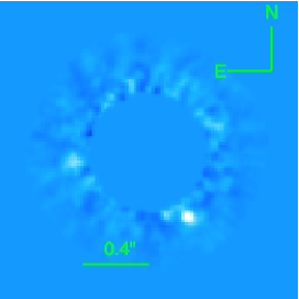
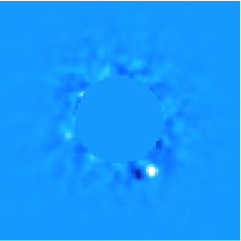
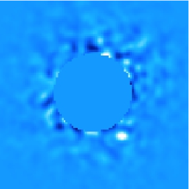
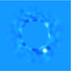
Figure 1.— Processed Gemini-NICI images obtained at $H$ band (top-left), $K_{s}$ band (top-right), and the $H_{2}0$ filter centered on $\sim$ 3.1 $\mu m$ (bottom panels: 23 Dec 2012 data on bottom-left, 26 Dec 2012 data on the bottom right). For clarity, we mask the region interior to $\sim$ 0$\farcs$4 and convolve the image with a gaussian equal to the image FWHM. The planet $\beta$ Pic b is in the lower-right at a position angle of $\sim$ 210^o and a separation of $\sim$ 0$\farcs$46. The color scale is set such that over the planet’s FWHM the pixel color is white.

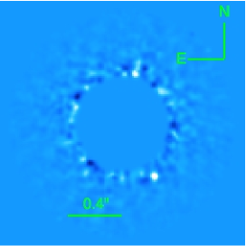
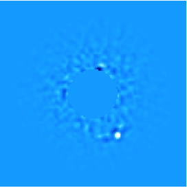
Figure 2.— Processed VLT/NaCo $J$ (left) and $H$ (right) band images presented in the same manner as Figure 1. Owing to very good speckle suppression, the $H$-band data’s effective inner working angle beyond which we are sensitive to $\beta$ Pic b-brightness companions is significantly smaller than for the $J$ band data and the preceding NICI images ($r_{IWA}$ = 0$\farcs$2).

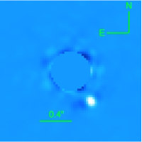
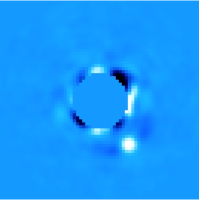
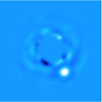
Figure 3.— Processed VLT/NaCo $L^{\prime}$ (left), [4.05] (middle), and $M^{\prime}$ (right) images presented as in Figures 1 and 2.

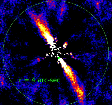
Figure 4.— Classical ADI reduction of our $L^{\prime}$ data showing a clear detection of the $\beta$ Pic debris disk. The green dot denotes the position of $\beta$ Pic b in the disk.

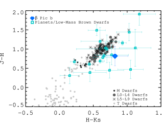
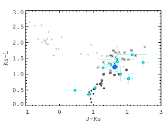
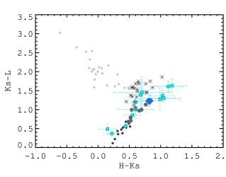
Figure 5.— Near-to-mid infrared color-color diagrams comparing $\beta$ Pic b’s colors (blue diamonds) to those of M dwarfs (small dark circles), early L-type brown dwarfs (grey circles), late L dwarfs (asterisks), and T dwarfs (light grey dots) from Leggett et al. (2010). We also overplot the positions of young, substellar objects/other directly-imaged planets (turquoise squares).

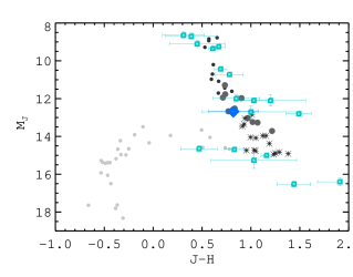
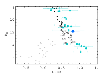
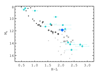
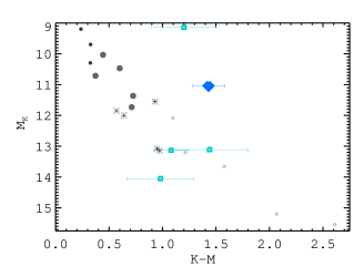
Figure 6.— Color-magnitude diagrams comparing $\beta$ Pic b to field M, L, and T dwarfs and young, substellar objects. Symbols are the same as in Figure 5.

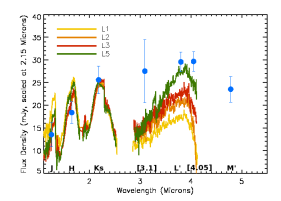
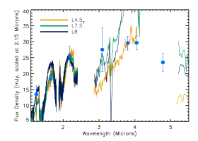
Figure 7.— Photometric data for $\beta$ Pic b compared to L dwarf standard spectra between L2 and L8 as well as a low surface gravity L4 dwarf from Cushing et al. (2005, 2008). We scale $\beta$ Pic b’s flux density at $K_{s}$ band to the band-integrated flux density of the standards at 2.15 $\mu m$. With the possible exception of the low surface gravity L4 dwarf, none of these standards provide a good match to measurments for $\beta$ Pic b. We identify the passbands along the bottom of the plot (left-hand panel).

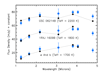
Figure 8.— Comparisons between the $\beta$ Pic b SED and the closest-matching substellar objects with $JHK_{s}L^{\prime}$ photometry. Quantitatively, 1RXJ 1609 B and $\kappa$ And b provide the closest matches, although it is as-yet unclear whether any known substellar object fully reproduces $\beta$ Pic b’s SED at all measured wavelengths.

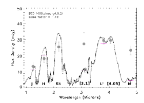
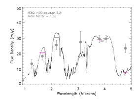
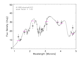
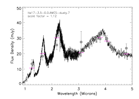
Figure 9.— The $\chi^{2}$ distributions (top-left) and best-fitting models (top-right, middle panels) for our limiting cases: the E60, thin cloud/large dust models the AE60, moderately-thick cloud/large dust models (second row), and the A60, thick cloud/large dust models. (Bottom panels) The $\chi^{2}$ distributions and best-fit AMES-DUSTY models which assume ISM-sized dust grains. The horizontal lines in the lefthand panels display the 68% and 95% confidence limits. The pink bars roughly denote the model-predicted flux densities at the filters’ central wavelength positions. We identify the passbands along the bottom of the plot (top-right panel).

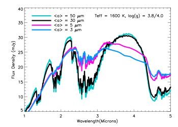
Figure 10.— The effect of atmospheric dust particle sizes on the shape of a massive planet SED. Here, the $<a>$ = 50, 30, and 5 $\mu m$ models depict log(g) = 4, $T_{eff}$ = 1600 $K$ models while the $<a>$ = 3 $\mu m$ model assumes log(g) = 3.8 and is scaled to match the luminosity of the $<a>$ = 5 $\mu m$ model. For small particle sizes, surface gravity signatures are weak and this parameter’s effect is primarily to change the flux scaling.

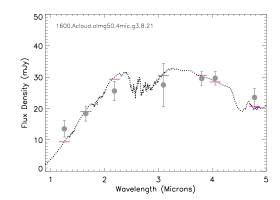
Figure 11.— The $\chi^{2}$ distribution (left) and best-fitting model (right) for the thick cloud, small dust A4 models, showing that we can achieve statistically significant fits to the data provided that the clouds are thick and the atmospheric dust particles are significantly smaller than those we have previously assumed in matching L dwarf spectra (c.f. Burrows et al., 2006). This model fitting ties the planet radius to predictions for hot-start models from Burrows et al. (1997). The horizontal dashed lines identify the 95% confidence limit (top) and 68% confidence limit (bottom).

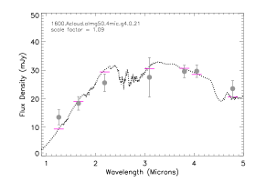
Figure 12.— Same as Figure 11 except treating the planet radius as a free parameter. Here we show the log(g) = 4, $T_{eff}$ = 1600 $K$, though the synthetic spectrum’s appearance and its agreement with the data at neighboring gridpoints in surface gravity is nearly identical.

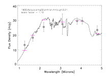
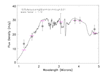
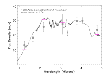
Figure 13.— SED fits adopting the nominally good-fitting atmosphere parameters depicted in Figure 12 but enhancing the atmosphere of methane.

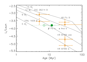
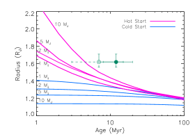
Figure 14.— (left) Luminosity evolution for hot-start models from Baraffe et al. (2003), comparing $\beta$ Pic b’s luminosity as derived in this work to that for the directly-imaged planets HR 8799 bcde, the planet/low-mass brown dwarf $\kappa$ And b, and other very low-mass brown dwarf companions. The solid circle denotes $\beta$ Pic b’s nominal positions, whereas the open circle identifies its effective position on this plot if it formed after 5 Myr. (Right) Evolution of the radius for planets with masses of 1–10 $M_{J}$ for the “hot-start” and “cold-start” planet cooling models from Spiegel and Burrows (2012). The radius error bars define the range of planet radii from models consistent with the data to within the 68% confidence limit.

References

- Allard et al. (2001) Allard, F., et al., 2001, ApJ, 556, 357
- Amara and Quanz (2012) Amara, A., Quanz, S., 2012, MNRAS, 427, 948
- Baraffe et al. (2003) Baraffe, I., et al., 2003, A&A, 402, 701
- Bailey et al. (2013) Bailey, V., Hinz, P., Currie, T., et al., 2013, ApJ, 767, 31
- Bejar et al. (2008) Bejar, V. J., et al., 2008, ApJ, 673, L185
- Beuzit et al. (2008) Beuzit, J.-L., et al., 2008, SPIE, 7014, 41
- Biller et al. (2010) Biller, B., et al., 2010, ApJ, 720, 82L
- Bitner et al. (2010) Bitner, M., et al., 2010, 714, 1542
- Boccaletti et al. (2013) Boccaletti, A., et al., 2013, A&A, 551, L14
- Bonnefoy et al. (2010) Bonnefoy, M., et al., 2010, A&A, 512, 52
- Bonnefoy et al. (2011) Bonnefoy, M., et al., 2011, A&A, 528, 15L
- Bonnefoy et al. (2013) Bonnefoy, M., et al., 2013a, A&A, 555, 107
- Bowler et al. (2010) Bowler, B., et al., 2010, ApJ, 733, 850
- Bowler et al. (2011) Bowler, B., et al., 2011, ApJ, 743, 148
- Bromley and Kenyon (2011) Bromley, B., Kenyon, S. J., 2011, ApJ, 731, 101
- Burgasser et al. (2013) Burgasser, A., et al., 2013, ApJ submitted, arXiv:1303.7283
- Burrows et al. (1997) Burrows, A., et al., 1997, ApJ, 491, 856
- Burrows et al. (2006) Burrows, A., et al., 2006, ApJ, 640, 1063
- Carson et al. (2013) Carson, J., et al., 2013, ApJ, 763, L32
- Chauvin et al. (2004) Chauvin, G., et al., 2004, A&A, 425, 29L
- Chauvin et al. (2005) Chauvin, G., et al., 2005, A&A, 438, L29
- Chauvin et al. (2012) Chauvin, G., et al., 2012, A&A, 542, 41
- Cohen et al. (1995) Cohen, M., et al., 1995, AJ, 110, 275
- Cohen et al. (2003) Cohen, M, et al., 2003, AJ, 126, 1090
- Currie et al. (2007) Currie, T., et al., 2007, 669, L33
- Currie et al. (2009) Currie, T., Lada, C. J, et al., 2009, ApJ, 698, 1
- Currie et al. (2010) Currie, T., Bailey, V., et al., 2010, ApJ, 721, L177
- Currie et al. (2011a) Currie, T., Burrows, A., et al., 2011, ApJ, 729, 128
- Currie et al. (2011b) Currie, T., Thalmann, C., et al., 2011, ApJ, 736, L33
- Currie and Sicilia-Aguilar (2011) Currie, T., Sicilia-Aguilar, A., 2011, ApJ, 732, 24
- Currie et al. (2012a) Currie, T., et al., 2012a, ApJ, 760, L32
- Currie et al. (2012b) Currie, T., et al., 2012b, ApJ, 755, L34
- Currie et al. (2012c) Currie, T., et al., 2012c, ApJ, 757, 28
- Cushing et al. (2005) Cushing, M., et al., 2005, ApJ, 623, 1115
- Cushing et al. (2008) Cushing, M., et al., 2008, ApJ, 678, 1372
- Dawson et al. (2011) Dawson, R., et al., 2011, ApJ, 743, L17
- Deirmendjian (1964) Deirmendjian, D., 1964, Appl. Opt., 3, 87
- Delorme et al. (2013) Delorme, P., et al., 2013, A&A, 553, L5
- Fabrycky and Murray-Clay (2010) Fabrycky, D., Murray-Clay, R., 2010, ApJ, 710, 1408
- Fedele et al. (2010) Fedele, D., et al., 2010, A&A, 510, 72
- Fortney et al. (2008) Fortney, J., et al., 2008, ApJ, 683, 1104
- Galicher et al. (2011) Galicher, R., et al., 2011, ApJ, 739, L41
- Galicher et al. (2013) Galicher, R., Marois, C., et al., 2013, in prep.
- Girard et al. (2012) Girard, J, et al., 2012, in Society of Photo-Optical Instrumentation Engineers (SPIE) Conference Series, Vol. 8447, Society of Photo-Optical Instrumentation Engineers (SPIE) Conference Series
- Golimowski et al. (2006) Golimowski, D., et al., 2006, AJ, 131, 3109
- Hauschildt and Baron (1999) Hauschildt, P., Baron, E., 1999, JCAM, 109, 41
- Hubeny and Burrows (2007) Hubeny, I., Burrows, A., 2007, ApJ, 669, 1248
- Ireland et al. (2011) Ireland, M., et al., 2011, ApJ, 726, 113
- Jaffe et al. (2006) Jaffe, D., et al., 2006, SPIE, 6269, 166
- Kenyon and Bromley (2009) Kenyon, S., Bromley, B., 2009, ApJ, 690, L140
- Konopacky et al. (2013) Konopacky, Q., et al., 2013, Science, 339, 1398
- Kratter et al. (2010) Kratter, K., et al., 2010, ApJ, 710, 1375
- Kraus and Ireland (2012) Kraus, A., Ireland, M., 2012, ApJ, 745, 1
- Lafrenière et al. (2007a) Lafreniére, D., et al., 2007a, ApJ, 670, 1367
- Lafrenière et al. (2007b) Lafreniére, D., et al., 2007b, ApJ, 660, 770
- Lafreniére et al. (2008) Lafreniére, D., et al., 2008, ApJ, 689, L153
- Lafrenière et al. (2010) Lafreniére, D., et al., 2010, ApJ, 719, 497
- Lagrange et al. (2009a) Lagrange, A.-M., et al., 2009, A&A, 493, L21
- Lagrange et al. (2010) Lagrange, A.-M., et al., 2010, Science, 329, 57
- Lagrange et al. (2012a) Lagrange, A.-M., et al., 2012a, A&A, 542, L18
- Lagrange et al. (2012b) Lagrange, A.-M., et al., 2012b, A&A, 542, L40
- Leggett et al. (2010) Leggett, S., et al., 2010, ApJ, 710, 1627
- Lowrance et al. (1999) Lowrance, P., et al., 1999, ApJ, 512, L69
- Lowrance et al. (2000) Lowrance, P., et al., 2000, ApJ, 541, 390
- Luhman et al. (2007) Luhman, K. L., et al., 2007, ApJ, 654, 570
- Luhman et al. (2013) Luhman, K. L., 2013, ApJ, 767, L1
- Macintosh et al. (2008) Macintosh, B., et al., 2008, SPIE, 7015, 31
- Madhusudhan et al. (2011) Madhusudhan, N., Burrows, A., Currie, T., 2011, ApJ, 737, 34
- Marois et al. (2006) Marois, C., et al., 2006, ApJ, 641, 556
- Marois et al. (2008) Marois, C., et al., 2008, Science, 322, 1348
- Marois et al. (2010a) Marois, C., et al., 2010a, Nature, 468, 1080
- Marois et al. (2010b) Marois, C., et al., 2010b, SPIE, 7736, 52
- Martinache et al. (2009) Martinache, F., Guyon, O., 2009, SPIE, 7440, 20
- Oberg et al. (2011) Oberg, K., et al., 2011, ApJ, 743, L16
- Pascucci et al. (2006) Pascucci, I., et al., 2006, ApJ, 651, 1177
- Pecaut et al. (2012) Pecaut, M., et al., 2012, ApJ, 746, 154
- Quanz et al. (2010) Quanz, S., et al., 2010, ApJ, 722, L49
- Rafikov (2011) Rafikov, R., 2011, ApJ, 727, 86
- Rameau et al. (2013) Rameau, J., et al., 2013, A&A, 553, 60
- Rayner et al. (2009) Rayner, J., et al., 2009, ApJS, 185, 289
- Rieke et al. (2008) Rieke, G. H., et al., 2008, AJ, 135, 2245
- Rodigas et al. (2012) Rodigas, T. J., et al., 2012, ApJ, 752, 57
- Rousset et al. (2003) Rousset, G., et al., 2003, SPIE 4839, 140
- Skemer et al. (2011) Skemer, A., et al., 2011, ApJ, 732, 107
- Skemer et al. (2012) Skemer, A., et al., 2012, ApJ, 753, 14
- Soummer et al. (2012) Soummer, R., Pueyo, L., Larkin, J., 2012, ApJ, 755, L28
- Spiegel and Burrows (2012) Spiegel, D., Burrows, A., 2012, ApJ, 745, 174
- Sudol and Haghighipour (2012) Sudol, J., Haghighighpour, N., 2012, ApJ, 755, 38
- Thalmann et al. (2009) Thalmann, C., et al., 2009, ApJ, 707, L123
- Tokunaga and Vacca (2005) Tokunaga, A., Vacca, W. D., 2005, PASP, 117, 421
- Vigan et al. (2012) Vigan, A., et al., 2012, A&A, 544, 9
- Wahhaj et al. (2011) Wahhaj, Z., et al., 2011, ApJ, 729, 139
- Whitney et al. (2003) Whitney, B., et al., 2003, ApJ, 598, 1079
- Zuckerman et al. (2001) Zuckerman, B., et al., 2001, ApJ, 562, L87