Detection of ¹⁵NNH⁺ in L1544: non-LTE modelling of dyazenilium hyperfine line emission and accurate ¹⁴N/¹⁵N values

Abstract

Context. Samples of pristine Solar System material found in meteorites and interplanetary dust particles are highly enriched in ${}^{15}\mathrm{N}$. Conspicuous nitrogen isotopic anomalies have also been measured in comets, and the ${}^{14}\mathrm{N}$/${}^{15}\mathrm{N}$ abundance ratio of the Earth is itself larger than the recognised pre-solar value by almost a factor of two. Ion–molecules, low-temperature chemical reactions in the proto-solar nebula have been repeatedly indicated as responsible for these ${}^{15}\mathrm{N}$-enhancements.

Aims. We have searched for ${}^{15}\mathrm{N}$ variants of the $\mathrm{N}_{2}\mathrm{H}^{+}$ ion in L1544, a prototypical starless cloud core which is one of the best candidate sources for detection owing to its low central core temperature and high CO depletion. The goal is the evaluation of accurate and reliable ${}^{14}\mathrm{N}$/${}^{15}\mathrm{N}$ ratio values for this species in the interstellar gas.

Methods. A deep integration of the ${}^{15}\mathrm{NNH}^{+}$$\>(1-0)$ line at 90.4 GHz has been obtained with the IRAM 30 m telescope. Non-LTE radiative transfer modelling has been performed on the $J=1-0$ emissions of the parent and ${}^{15}\mathrm{N}$-containing dyazenilium ions, using a Bonnor–Ebert sphere as a model for the source.

Results. A high-quality fit of the $\mathrm{N}_{2}\mathrm{H}^{+}$ (1–0) hyperfine spectrum has allowed us to derive a revised value of the $\mathrm{N}_{2}\mathrm{H}^{+}$ column density in L1544. Analysis of the observed $\mathrm{N}^{15}\mathrm{NH}^{+}$ and ${}^{15}\mathrm{NNH}^{+}$ spectra yielded an abundance ratio $N(\mathrm{N}^{15}\mathrm{NH}^{+})/N(^{15}\mathrm{NNH}^{+})=1.1\pm 0.3$. The obtained ${}^{14}\mathrm{N}$/${}^{15}\mathrm{N}$ isotopic ratio is $\sim 1000\pm 200$, suggestive of a sizeable ${}^{15}\mathrm{N}$ depletion in this molecular ion. Such a result is not consistent with the prediction of present nitrogen chemical models.

Conclusions. As chemical models predict large ${}^{15}\mathrm{N}$ fractionation of $\mathrm{N}_{2}\mathrm{H}^{+}$, we suggest that ${}^{15}\mathrm{N}$${}^{14}\mathrm{N}$, or ${}^{15}\mathrm{N}$ in some other molecular form, is preferentially depleted onto dust grains.

1 Introduction

Determination of the abundance ratios of the stable isotopes of the light elements in different objects of the Solar System is one of the key elements to understand its origin and early history (see, e.g. Caselli & Ceccarelli 2012). Nitrogen, the fifth or sixth most abundant element in the Sun (after H, He, C, O, and maybe Ne, Asplund et al. 2009), is particularly intriguing because its isotopic composition shows large variations whose interpretation is still controversial (Aléon 2010; Adande & Ziurys 2012).

Recent laboratory analysis of the solar wind particles collected by the Genesis spacecraft (Marty et al. 2011) yielded a ${}^{14}\mathrm{N}$/${}^{15}\mathrm{N}$ ratio of $441\pm 6$, higher than in any Solar System object, but probably representative of the proto-solar nebula value, being comparable to that measured in Jupiter’s atmosphere ($435\pm 57$, Owen et al. 2001; Fouchet et al. 2004) and in osbornite (TiN) calcium-aluminium-rich inclusion from the CH/CB chondrite Isheyevo ($424\pm 3$, Meibom et al. 2007). The ${}^{14}\mathrm{N}$/${}^{15}\mathrm{N}$ value of the terrestrial atmosphere is significantly lower ($\sim 272$), and larger ${}^{15}\mathrm{N}$ enrichments were measured in cometary nitrile-bearing molecules (Arpigny et al. 2003; Bockelée-Morvan et al. 2008; Manfroid et al. 2009) and in primitive chondritic materials (up to 50, e.g., Briani et al. 2009; Bonal et al. 2010).

A common but still debated interpretation considers such variations as an inheritance of the proto-solar chemistry: low-temperature ion–molecule reactions (e.g., Millar 2002) in the interstellar medium (ISM) were proven to cause large isotopic excesses for D in organic molecules, and have repeatedly been proposed as the cause of the observed ${}^{15}\mathrm{N}$ excesses too. However, in molecular clouds, gas-phase chemistry continually cycles nitrogen between atomic and molecular forms, equating the composition of the isotopic reservoirs. Indeed, classical ion–molecule reaction models fail to predict major ${}^{15}\mathrm{N}$ enrichments (Terzieva & Herbst 2000). Specific conditions, such as strong and selective CO freeze-out (Charnley & Rodgers 2002; Rodgers & Charnley 2008), might overcome this difficulty and produce a “nitrogen super-fractionation” in cold ISM, capable in principle to account for the largest measured enhancements.

A way to assess the isotopic composition of the pre-solar gas is the measurements of the ${}^{14}\mathrm{N}$/${}^{15}\mathrm{N}$ ratio in other proto-stellar systems. Recent observations of ${}^{15}\mathrm{N}$-bearing molecules found no significant fractionation in NH₃ (${}^{14}\mathrm{N}/^{15}\mathrm{N}=350-500$, Gerin et al. 2009; $334\pm 50$, Lis et al. 2010) toward pre-stellar cores and proto-stellar envelopes, and in $\mathrm{N}_{2}\mathrm{H}^{+}$ (${}^{14}\mathrm{N}/^{15}\mathrm{N}=446\pm 71$, Bizzocchi et al. 2010) toward the prototypical starless cloud core L1544. Conversely, various preliminary measurements on nitrile species towards pre-stellar cores showed that they are highly enriched in ${}^{15}\mathrm{N}$ (between 70 and 380, Milam & Charnley 2012; Hily-Blant et al. 2013; Bizzocchi unpublished). Also, similar values have been found by Adande & Ziurys (2012) in HNC observations of massive star-forming regions across the Galaxy.

Another problem to directly link pre-stellar core chemistry and the Solar System composition comes from the poor correlation between D- and ${}^{15}\mathrm{N}$-enhancements observed in some pristine materials (Busemann et al. 2006; Robert & Derenne 2006), whereas it is clear that the chemical processes invoked to account for nitrogen fractionation should also produce enormous deuterium enhancements.

Wirström et al. (2012) considered the spin-state dependence in ion–molecule reactions involving the ortho and para forms of H₂ and succeeded in reproducing the differential ${}^{15}\mathrm{N}$-fractionation observed in amine- and nitrile-bearing compounds, as well as the overall lack of correlation with hydrogen isotopic anomalies. The authors pointed out that, in cold interstellar environments, the ortho-to-para ratio of H₂ plays a pivotal role in producing a diverse range of D–${}^{15}\mathrm{N}$ fractionation in precursors molecules, thus providing a strong support for the astrochemical origin of nitrogen isotopic anomalies. However, this hypothesis still requires a sound verification since so far, observations of ${}^{15}\mathrm{N}$-isotopologues in the ISM are rather sparse. An extended survey of the ${}^{14}\mathrm{N}$/${}^{15}\mathrm{N}$ ratio targeting starless clouds in different evolutionary phases, and possibly in different environmental conditions, is thus desirable.

Obtaining accurate determinations of the nitrogen isotopic ratio in the ISM is problematic: ${}^{15}\mathrm{N}$-bearing species produce typically very weak emissions, which requires time consuming high sensitivity observations. Moreover, the rotational spectra of common N-containing species are usually optically thick and the line intensities are not reliable indicators of the molecular abundance. For nitrile molecules, this latter difficulty may be overcome using less abundant ${}^{13}\mathrm{C}$ variants as proxies for the parent species and then deriving the ${}^{14}\mathrm{N}$/${}^{15}\mathrm{N}$ ratio from an assumption for the ${}^{12}\mathrm{C}$/${}^{13}\mathrm{C}$ (e.g., Dahmen et al. 1995). Another route is to use the hyperfine structure analysis to evaluate the optical depth of the parent species, thus allowing for a more direct determination of the nitrogen isotope ratio (Savage et al. 2002; Adande & Ziurys 2012).

In a previous letter, Bizzocchi et al. (2010) reported the detection of $\mathrm{N}^{15}\mathrm{NH}^{+}$ in L1544. The analysis was carried out assuming local thermodynamic equilibrium (LTE) conditions and yielded a ${}^{14}\mathrm{N}$/${}^{15}\mathrm{N}$ ratio of $446\pm 71$. This is indicating the absence of nitrogen fractionation in the dyazenilium ion, a result not consistent with the prediction of the chemical model of Gerin et al. (2009) and Wirström et al. (2012).

The chosen target, L1544, is a prototypical starless core on the verge of the star-formation (Ward-Thompson et al. 1999; Caselli et al. 2002a). Its density structure, low central temperature, and high CO depletion make it an ideal laboratory to study the isotopic fractionation processes. Also, an accurate model for its internal structure and dynamics has been proposed by Keto & Caselli (2010) and then successfully used to analyse the H₂O emission observed by Herschel (Caselli et al. 2012). In this paper we present the detection of ${}^{15}\mathrm{NNH}^{+}$ isotopologue in L1544 together with a full non-LTE radiative transfer treatment of the dyazenilium ions aimed at the evaluation of accurate and reliable values of the ${}^{14}\mathrm{N}$/${}^{15}\mathrm{N}$ ratio in this species.

The paper is organised as follows: in § 2 we describe the technique used for observations, and in § 3 we summarise our direct observational results. § 4 is devoted to the description of the Monte Carlo radiative transfer modelling of $\mathrm{N}_{2}\mathrm{H}^{+}$ and its ${}^{15}\mathrm{N}$-variants, and the derivation of their molecular abundances. In § 5 we discuss the implications for the chemical models and in § 6 we summarise our conclusions.

2 Observations

The observations towards L1544 were carried out with the IRAM 30 m antenna, located at Pico Veleta (Spain) during observing sessions in June 2009 and July 2010. The $J=1-0$ transition of ${}^{15}\mathrm{NNH}^{+}$ was observed with the EMIR receiver in the E090 configuration tuned at 90 263.8360 MHz and using the lower-inner side-band. The hyperfine-free rest frequencies were taken from the most recent laboratory investigation of ${}^{15}\mathrm{N}$-dyazenilium species (Dore et al. 2009). Scans were performed in frequency switching mode, with a throw of $\pm$7 MHz; the backend used was the VESPA correlator set to a spectral resolution of 20 kHz (corresponding to 0.065 km s^-1) and spectral bandpass of 20 MHz. We tracked the L1544 continuum dust emission peak at 1.3 mm, where we previously detected the other ${}^{15}\mathrm{N}$-containing isotopologue, $\mathrm{N}^{15}\mathrm{NH}^{+}$ (Bizzocchi et al. 2010). The J2000 coordinates are: $\mathrm{RA}=05^{\mathrm{h}}04^{\mathrm{m}}17.21^{\mathrm{s}}$, $\mathrm{Dec}=25^{\circ}10^{\prime}42.8^{\prime\prime}$ (Caselli et al. 2002a). The telescope pointing was checked every two hours on nearby bright radio quasars and was found accurate to 3–4″; the half power beam width (HPBW) at the line frequency is 27″.

In may 2009 we spent 4.25 hours on source with average atmospheric condition ($\tau\sim 0.1$), while during the summer 2010 session we observed for further 23.9 hours with good weather conditions ($\tau<0.05$); all those scans were summed together for a total of 28.15 hours of on-source telescope time. Horizontal and vertical polarizations were simultaneously observed and averaged together to produce the final spectrum, which was then rescaled in units of $T_{\mathrm{mb}}$ assuming a source filling factor of unity and using the forward and main beam efficiencies appropriate for $91\,\mathrm{GHz}$: $F_{\mathrm{eff}}=0.95$ and $B_{\mathrm{eff}}=0.75$, respectively. The rms noise level achieved was about 3 mK, close to that obtained for the $J=1-0$ line of the species $\mathrm{N}^{15}\mathrm{NH}^{+}$ toward the same line of sight (Bizzocchi et al. 2010).

The same backend configuration was also employed to collect new data for the $J=1-0$ transition of the main isotopologue, $\mathrm{N}_{2}\mathrm{H}^{+}$, with the EMIR receiver tuned at 93 173.4013 MHz. This line was observed shortly at the beginning of each telescope session for a total integration time of $\sim$56 min. The final rms noise level is 15 mK, resulting in a high signal-to-noise spectrum, well suited for modelling purposes.

Table 1: Predicted hyperfine frequencies, estimated $1\sigma$ uncertainties, and relative line intensities for the $J=1-0$ transition of $\mathrm{N}^{15}\mathrm{NH}^{+}$ and ${}^{15}\mathrm{NNH}^{+}$ (Dore et al. 2009).

Isotopologue	$F^{\prime}-F$	Frequency	Uncertainty	Relative intensity
		(MHz)	(kHz)
$\mathrm{N}^{15}\mathrm{NH}^{+}$	1 - 1	$91\,204.2602$	$0.9$	$1.000$
	2 - 1	$91\,205.9908$	$0.8$	$1.667$
	0 - 1	$91\,208.5162$	$1.2$	$0.333$
${}^{15}\mathrm{NNH}^{+}$	1 - 1	$90\,263.4870$	$0.9$	$1.000$
	2 - 1	$90\,263.9120$	$0.6$	$1.667$
	0 - 1	$90\,264.4972$	$1.6$	$0.333$

Table 2: Results of the CLASS HFS fit on the observed spectral profile of the ${}^{15}\mathrm{N}$-bearing dyazenilium isotopologues observed towards L1544. Numbers in parentheses refer to $1\sigma$ uncertainties in units of the last quoted digit.

Line	Rest frequencya	$A$ coefficientb	$v_{LSR}$	$\int T_{\mathrm{mb}}\mathrm{d}v$ c	$\Delta v$ d
	(MHz)	$10^{5}\,$s-1	(km s-1)	(mK km s-1)	(km s-1)
$\mathrm{N}^{15}\mathrm{NH}^{+}$ (1–0)	$91\,205.6945$	$3.19(32)$	$7.299(14)$	$21.4(22)$	0.507(43)
${}^{15}\mathrm{NNH}^{+}$ (1-0)	$90\,263.8354$	$3.42(35)$	$7.203(10)$	$18.3(13)$	0.409(21)

• From Dore et al. (2009).

• Calculated through Eq. (5) of Dore et al. (2009) and using the data of the same paper.

• Integrated intensity summed over all the components.

• Gaussian FWHM. Assumed equal for all the components.

Figure 1: Spectra of the ${}^{15}\mathrm{N}$-containing dyazenilium isotopologues observed towards L1544 (black histogram), and computed spectral profiles resulting from the HFS fits (red dashed curves). Superimposed black lines indicate the position and relative intensity of the hyperfine components. Left panel: $\mathrm{N}^{15}\mathrm{NH}^{+}$ (1–0) transition (reproduced from Bizzocchi et al. 2010). Right panel: ${}^{15}\mathrm{NNH}^{+}$ (1–0) transition, observed in July 2010 at IRAM 30m. The rms noise level is 2.6 mK.

3 Results

The two ${}^{15}\mathrm{N}$-dyazenilium spectra observed in L1544 are presented in Figure 1. Due to the smaller magnitude of the electric quadrupole coupling constant or the inner ${}^{14}\mathrm{N}$ atom, the hyperfine triplet of the ${}^{15}\mathrm{NNH}^{+}$ (1–0) transition is spread over $\sim 1$ MHz, much less than the other ${}^{15}\mathrm{N}$-isotopologue. For the sake of completeness, the frequencies and relative intensities of the $J=1-0$ hyperfine transition of both ${}^{15}\mathrm{N}$-bearing dyazenilium variants are reported in Table 1 (Dore et al. 2009).

The data were processed using the GILDAS software (Pety 2005). After polynomial baseline subtraction, average line parameters were estimated by fitting Gaussian line profiles to the detected components using the HFS routine implemented in CLASS. The hyperfine splittings and relative intensities of the $J=1-0$ transitions of both ${}^{15}\mathrm{N}$ isotopologues were taken from Table 1 and kept fixed in the least-squares procedure. Since the lines are optically thin within the HFS fitting errors, we forced the optical depth to have the value of 0.1, the minimum allowed in CLASS. This method has been adopted in the past (e.g., Caselli et al. 2002b) to avoid highly uncertain values of the optical depth to affect the intrinsic line width, as the error on $\tau$ is not propagated in the evaluation of the line width.

The derived parameters for ${}^{15}\mathrm{NNH}^{+}$ (1–0) are gathered in Table 2, where the results obtained from the previous $\mathrm{N}^{15}\mathrm{NH}^{+}$ (1–0) observations are also reported for completeness. From these data one can derive a systemic velocity $V_{\mathrm{LSR}}=7.203\pm 0.010$ km s^-1 for ${}^{15}\mathrm{NNH}^{+}$ (1–0) which compares well with the value derived previously for the $\mathrm{N}^{15}\mathrm{NH}^{+}$ (1–0), i.e., $V_{\mathrm{LSR}}=7.299\pm 0.014$ km s^-1 (Bizzocchi et al. 2010). The small discrepancies observed in source velocity and in the line width between the ${}^{15}\mathrm{N}$-species (these quantities agrees within 5$\sigma$), are likely to be attributed to the low signal-to-noise ratio and the spectral resolution (0.067 km s^-1).

4 L1544 modelling and radiative transfer

In the following subsections we describe the radiative transfer treatment carried out on L1544 to model the $J=1-0$ emission of $\mathrm{N}_{2}\mathrm{H}^{+}$, $\mathrm{N}^{15}\mathrm{NH}^{+}$, and ${}^{15}\mathrm{NNH}^{+}$, and to derive accurate molecular abundances and ${}^{14}\mathrm{N}/^{15}\mathrm{N}$ ratios. The physical model is based on that proposed by Keto & Caselli (2010) and updated with the inclusion of oxygen to interpret the far infrared emission of the water vapour in the same source (Caselli et al. 2012). Briefly, the core is described as a gravitationally contracting Bonnor–Ebert sphere; the model includes radiative equilibrium from dust, gas cooling via both molecular emission lines and grain collisional coupling, as well as a simplified molecular chemistry (Keto & Caselli 2008).

First, we used the original model with a central density of $2\times 10^{7}$ cm^-3: its temperature, density, and inward velocity profile are shown in Figure 2. The H₂ column density, averaged over the 30 m telescope main beam FWHM at 3 mm, is $6.57\times 10^{22}$ cm^-2. This value compares well with that derived by Crapsi et al. (2005) through dust continuum emission observation at 1.2 mm; once averaged over the same beam (11″), our model yields $11.5\times 10^{22}$ cm^-2, consistent with the observed value of $(9.4\pm 1.6)\times 10^{22}$ cm^-2.

The radiative transfer calculations have been performed using the non-local thermodynamic equilibrium (non-LTE) numerical code MOLLIE (Keto 1990; Keto et al. 2004). We used here the updated version of the algorithm, able to treat in a proper way the issue of overlapping lines, thus allowing to better reproduce the non-LTE hyperfine ratios (excitation anomalies) observed in the $\mathrm{N}_{2}\mathrm{H}^{+}$ spectra of L1544 and in a number of other starless cores (Caselli et al. 1995; Daniel et al. 2007). For the present modelling we mostly relied on the hyperfine rates calculations of Daniel et al. (2004, 2005) for $\mathrm{N}_{2}\mathrm{H}^{+}$/He collisions; appropriate rate coefficients for H₂ partner were then obtained using a suitable scaling relation (see Appendix A).

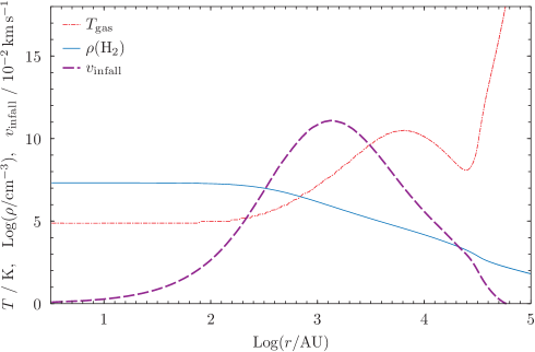
Figure 2: Temperature, density, and inward velocity profiles of L1544 used as model in the present radiative transfer modelling. The red dotted curve indicates the gas temperature in K, the blue curve is the log of density in cm^-3, and the purple dashed curve represents the inward velocity in units of 0.01 km s^-1.

The cloud structure of L1544 was modelled with 3 nested grids, each composed of 48 cells. The cell linear dimensions of each nested level are decreasing, i.e., the level 1 covers the whole source out to a radius of 66 000 AU, whereas the finer level 3 maps the inner 16 000 AU of the core. In each cell, the temperature, density, and gas kinematic parameters were taken from the model shown in Figure 2 and assumed constant. A constant turbulent FWHM line width of 0.13 km s^-1 (as found by Tafalla et al. 2002) was added in quadrature to the thermal line width calculated in each model cell.

4.1 N₂H⁺ (1–0)

Radiative transfer modelling of $\mathrm{N}_{2}\mathrm{H}^{+}$ is not an easy task. Because of the two ${}^{14}\mathrm{N}$ nuclei, each rotational level is split by quadrupole interactions into nine sub-levels and the rotational transitions exhibit a complex structure of hyperfine components (i.e., 15 for $J=1-0$, 38 for $J=2-1$, etc.) with various degrees of overlap between them. The presence of the hyperfine structure (HFS) complicates the modelling. The relative populations of the hyperfine sub-levels may depart from their statistical weights producing non-LTE intensity ratios (e.g., Caselli et al. 1995). Indeed, collisional coefficients for each individual hyperfine component typically have different values (e.g., Buffa 2012), thus producing hyperfine selective collisional excitation (Stutzki & Winnewisser 1985). A second effect is the “hyperfine line-trapping”, i.e., various components may have different optical depth, thus getting different amounts of radiative excitation. The trapping becomes important at high optical depths and is accentuated by the overlap of the various hyperfine components.

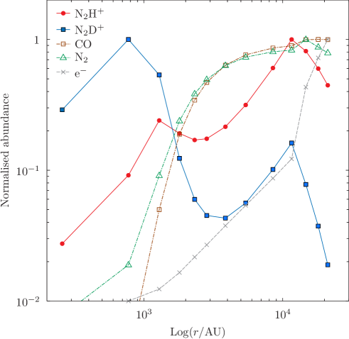
Figure 3: Abundance trends (normalised to the maximum values) predicted by the Aikawa et al. (2011) models for dyazenilium and chemically related species. The $\mathrm{N}_{2}\mathrm{H}^{+}$ abundance decreases toward the cloud centre following the N₂ freeze-out (green curve) onto dust mantels at high gas density. The concomitant steeper drops of free electron (grey curve) and CO (brown curve) give rise to the $\mathrm{N}_{2}\mathrm{H}^{+}$ abundance maxima at radii of $\sim 10^{4}$ and $\sim 10^{3}$ astronomical units. $\mathrm{N}_{2}\mathrm{D}^{+}$ shows a similar behaviour (blue curve) but it features a much stronger inner peak owing to the large deuterium fractionation existing in the highly–CO depleted central region.

A Monte Carlo modelling of the $\mathrm{N}_{2}\mathrm{H}^{+}$ (1–0) emission line in L1544 and other starless cores has previously been performed by Tafalla et al. (2002). They adopted a simplified treatment in which the above mentioned effects are ignored: all the hyperfine sub-levels were assumed to be populated according to their statistical weights (no hyperfine selective collisional excitation was considered), and the hyperfine line trapping was neglected. To justify such a simple approach, it was argued that line trapping is only significant at very large optical depths and, in any case, non-LTE intensity effects involved typically only 10–15% of the emerging flux. For most sources this modelling provided $\mathrm{N}_{2}\mathrm{H}^{+}$ spectra in good agreement with observations but it yielded a less satisfactory result for L1544. Notably, the predicted spectrum was unable to reproduce the non-Gaussian line shape of the hyperfine lines which was attributed to the presence of two velocity components in the core (Tafalla et al. 1998). They were thus roughly modelled using a broader profile.

Another issue involves the $\mathrm{N}_{2}\mathrm{H}^{+}$ abundance profile. So far, the source model used in radiative transfer studies of L1544 assumed a constant $\mathrm{N}_{2}\mathrm{H}^{+}$ abundance throughout the source (Tafalla et al. 1998, 2002; Keto & Rybicki 2010). This hypothesis is reasonable, given the similarity between the observed L1544 dust continuum and $\mathrm{N}_{2}\mathrm{H}^{+}$ (1–0) emission maps (see, e.g. Tafalla et al. 2002). Also, the observed radial profiles of the integrated line emission intensity (see Fig. 2 of Caselli et al. 1999), show that the abundance behaviour of $\mathrm{N}_{2}\mathrm{H}^{+}$ is markedly different from that of CO, which is known to suffer considerable depletion at the high gas densities toward the core centre. However, Caselli et al. (2002b) suggested that a certain amount of nitrogen depletion is also expected in the dense gas, thus the dyazenilium abundance is also likely to show a drop toward the L1544 centre (see also Bergin et al. 2002).

Given the uncertainties in the spatial distribution of $\mathrm{N}_{2}\mathrm{H}^{+}$ (due to the poor spatial resolution), we investigated both constant and central-drop abundance profiles. In either instances, we ran a grid of models with varying standard $\mathrm{N}_{2}\mathrm{H}^{+}$ abundance, and sought the best fit of the observed line profiles.

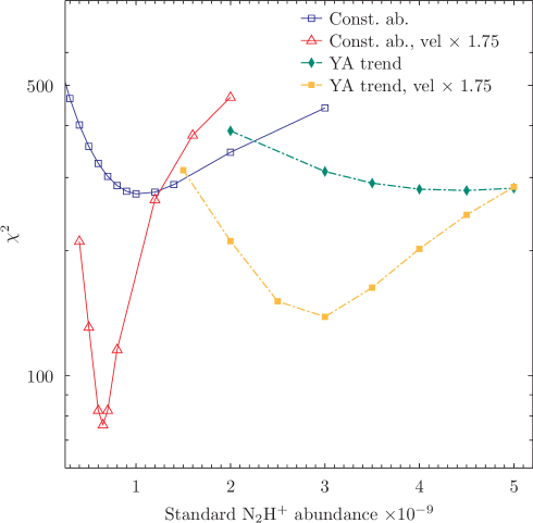
Figure 4: Weighted $\chi^{2}$ of the $\mathrm{N}_{2}\mathrm{H}^{+}$ (1–0) modellings using different standard dyazenilium abundances and radial profiles. Blue curve: constant $\mathrm{N}_{2}\mathrm{H}^{+}$ abundance with respect to H₂; red curve: constant abundance and modified cloud infall velocity (see text). Green curve: radial $\mathrm{N}_{2}\mathrm{H}^{+}$ abundance profile shown in Figure 3; yellow curve: radial profile with modified cloud infall velocity.

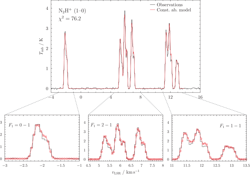
Figure 5: Observed $\mathrm{N}_{2}\mathrm{H}^{+}$ (1–0) spectrum in L1544 modelled with non-LTE code MOLLIE. The histograms show our observation data. The red curve shows the model spectrum computed using the “altered” dark cloud model and $\mathrm{N}_{2}\mathrm{H}^{+}$ constant abundance throughout the core (see text).

In the first set of models we used a constant dyazenilium abundance with respect to H₂, then we tested the $\mathrm{N}_{2}\mathrm{H}^{+}$ radial abundance profile calculated using the hydro-dynamical–chemical model of Aikawa et al. (2011). The employed chemical network is the same as in Aikawa et al. (2012), but not the dynamics. In this paper, we assume that the physical structure is fixed at the model shown in Figure 2 and the chemistry is run until the C¹⁸O column density reaches the observed value within the IRAM 30m beam. The predicted trends for a selection of chemical species are illustrated in Figure 3. Dyazenilium is formed by proton transfer to N₂ and destructed by reaction with CO and recombination with electron. As expected, the nitrogen freeze-out at smaller radii produces a overall decreasing $\mathrm{N}_{2}\mathrm{H}^{+}$ abundance trend, while the secondary peak at $\sim 1000$ AU is due to the concomitant faster drop of the main depleting reactants.

The “goodness” of each modelling was estimated using the quantity:

$$\chi^{2}=\sum_{i}^{N}\left\{\frac{1}{\sigma_{\mathrm{obs}}}\left[T_{\mathrm{mb,obs}}(i)-T_{\mathrm{mb,model}}(i)\right]\right\}^{2}\,,$$ (1)

where $T_{\mathrm{mb}}(i)$ are the brightness temperature of the observed and modelled spectra at the $i$-th velocity channel and $\sigma_{\mathrm{obs}}$ is the actual rms noise of the observation which is estimated to be 0.015 K. The sum in Eq. (1) run over all the velocity channels calculated by MOLLIE, covering an interval of 2 km s^-1 around each hyperfine component.

Figure 4 plots the resulting $\chi^{2}$ for varying standard $\mathrm{N}_{2}\mathrm{H}^{+}$ abundance and different abundance profiles. The blue and green curves represent the $\chi^{2}$ trends obtained adopting constant $\mathrm{N}_{2}\mathrm{H}^{+}$ abundance, and the radial $\mathrm{N}_{2}\mathrm{H}^{+}$ abundance profile shown in Figure 3, respectively. The two models yield fits of comparable but not satisfactory quality, as both fail in reproducing the observed brightness of the thinner $F_{1},F=(1,0)-(1,1)$ component. Another weakness of these simulations is the overall poor agreement of the spectral profile, i.e., the calculated lines are systematically narrower than the observed ones. This suggests that the inward velocity profile adopted as a model (see Figure 2) could be underestimated. In fact, the hydrodynamic calculations of Keto & Caselli (2010) result in idealised models of contracting Bonnor–Ebert spheres in quasi-static equilibrium and the contraction velocity was derived from noisier data.

We have thus altered L1544 cloud model by increasing its inward velocity profile by a constant factor, and sought again the minimum $\chi^{2}$ by varying the $\mathrm{N}_{2}\mathrm{H}^{+}$ standard abundance. Both constant and centrally decreasing $\mathrm{N}_{2}\mathrm{H}^{+}$ abundance profiles were tested. Best fits were obtained using a velocity profile scaled with a constant 1.75 factor; the resulting trends are illustrated by the red and yellow curves in Figure 4. A significant improvement was achieved for both profiles; the model with constant abundance drops to a narrow $\chi^{2}$ minimum of 76.2 and supersedes the best fit obtained with the centrally decreasing profile, which is almost twice poorer ($\chi^{2}\sim 140$). The obtained best $\chi^{2}$ for the two models correspond to weighted rms of 0.54 and 0.98, indicating that in both cases the observed profile is reproduced within the average spectral noise.

We regard the spectrum obtained with the constant $\mathrm{N}_{2}\mathrm{H}^{+}$ abundance profile and a standard abundance value of $6.5\times 10^{-10}$ as the “best-fit” model, this corresponds to the minimum of the red curve of Figure 4. The comparison between the observed and calculated $\mathrm{N}_{2}\mathrm{H}^{+}$ (1–0) spectral profiles is shown in Figure 5. The quality of the fit is remarkable: the double-peaked profile of all the hyperfine components is reproduced with high accuracy, including that of the weakest $F_{1},F=(1,0)-(1,1)$ line which exhibits only a minor asymmetry due to the low optical opacity. The $\mathrm{N}_{2}\mathrm{H}^{+}$ column density averaged over the IRAM 30 m main beam is $N=4.06\times 10^{13}$ cm^-2.

Figure 6 illustrates the optimal calculated $\mathrm{N}_{2}\mathrm{H}^{+}$ (1–0) spectrum adopting the centrally decreasing $\mathrm{N}_{2}\mathrm{H}^{+}$ abundance profile of Aikawa et al. (2011), and larger infall velocity (yellow curve in Figure 4). It can be seen that this modelling is also of reasonable quality, although the line profiles of the partially resolved velocity doublets is less well reproduced. For this model, the standard abundance value is $3.0\times 10^{-9}$ (value of 1 in Figure 3), yielding a $\mathrm{N}_{2}\mathrm{H}^{+}$ beam averaged column density of $N=3.32\times 10^{13}$ cm^-2.

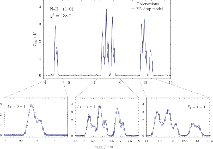
Figure 6: Observed $\mathrm{N}_{2}\mathrm{H}^{+}$ (1–0) spectrum in L1544 modelled with non-LTE code MOLLIE. The black histograms show our observation data. The blue curve shows the model spectrum computed using the “altered” dark cloud model and the $\mathrm{N}_{2}\mathrm{H}^{+}$ radial abundance profile of Aikawa et al. (2011).

Clearly, the values of $N(\mathrm{N}_{2}\mathrm{H}^{+})$ obtained through the above described method are affected by uncertainties that are difficult to evaluate. In principle, given the least-squares procedure adopted, one may derive the variance–covariance matrix of the system by evaluating the Jacobian of the optimised variables, i.e., the $\mathrm{N}_{2}\mathrm{H}^{+}$ standard abundance, the turbulent line-width, and the scaling factor applied to the hydro-dynamical velocity field.

Such a purely statistical procedure yields rather small errors ($<1$%), very likely to be negligible compared to the systematic uncertainties associated to the choice of the spherically-symmetric hydro-dynamical model — which we expect to be an over-simplified description of the real core structure — or to those produced by the inaccuracies of the collision data. To estimate the latter point, we ran various radiative transfer models, using artificially altered hyperfine rate coefficients by factors of 2 to 5. The resulting optimal $\mathrm{N}_{2}\mathrm{H}^{+}$ abundance showed only moderate changes (10-15%, 20% in the most extreme case), but the fits were systematically poorer ($\chi^{2}=200-300$) with the calculated spectral profile being increasingly unable to reproduce the observed infall asymmetry.

On the other hand, we have shown that one may adopt a completely different choice of $\mathrm{N}_{2}\mathrm{H}^{+}$ radial abundance profile still obtaining an acceptable fit (compare Figure 5 and  6), and this ultimately provides a mean to do an approximate evaluation of the $N(\mathrm{N}_{2}\mathrm{H}^{+})$ error bar. The column densities derived using different abundance profiles differ by $0.74\times 10^{13}$ cm^-2, i.e., 18% of our “best-fit” value. Assuming that this discrepancy represents the maximum $2\sigma$ dispersion of the actual $N(\mathrm{N}_{2}\mathrm{H}^{+})$, and adding in quadrature a conservative 10% calibration error, we ended with an estimated 13% relative uncertainty on the final results, $N(\mathrm{N}_{2}\mathrm{H}^{+})=(4.1\pm 0.5)\times 10^{13}$ cm^-2.

4.2 N¹⁵NH⁺ (1–0) and ¹⁵NNH⁺ (1–0)

Given the high quality fit to the $\mathrm{N}_{2}\mathrm{H}^{+}$ (1–0) hyperfine components, we adopt the velocity “augmented” L1544 model with constant molecular abundance to fit the observed spectra of the ${}^{15}\mathrm{N}$-containing isotopologues. Due to the lack of one ${}^{14}\mathrm{N}$ nucleus, the HFS of the $\mathrm{N}^{15}\mathrm{NH}^{+}$ (1–0) and ${}^{15}\mathrm{NNH}^{+}$ (1–0) lines are simpler than that of the parent species, i.e. they consist of triplets of hyperfine components. In addition, owing to the different quadrupole coupling constants, the $\mathrm{N}^{15}\mathrm{NH}^{+}$ (1–0) HFS is spread over 4.2 MHz (14 km s^-1), whereas the $\mathrm{N}^{15}\mathrm{NH}^{+}$ (1–0) triplet are contained in a $\sim 1$ MHz (3.3 km s^-1) interval.

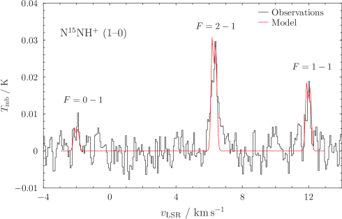
Figure 7: Observed $\mathrm{N}^{15}\mathrm{NH}^{+}$ (1–0) spectrum in L1544 modelled with non-LTE code MOLLIE. The black histogram shows our observation data. The red curve shows the model spectrum computed using the best fit model (see text).

The best simulations of the two lines were obtained by varying independently the $\mathrm{N}^{15}\mathrm{NH}^{+}$ and ${}^{15}\mathrm{NNH}^{+}$ standard abundance until the minimum $\chi^{2}$ is achieved. The best fit dyazenilium abundances are $6.2\times 10^{-13}$ and $6.0\times 10^{-13}$, for $\mathrm{N}^{15}\mathrm{NH}^{+}$ and ${}^{15}\mathrm{NNH}^{+}$, respectively.

The fit results are shown in Figure 7 and 8. The model computed spectra are characterised by symmetrical line profiles; they also show a small but well apparent velocity doubling as expected in the case of a contracting centrally concentrated core. However, the signal-to-noise ratio (SNR) achieved by the present observations is not enough to reveal this feature in the L1544 spectra. The low SNR plus the background effects are responsible for the peculiar line profile asymmetry exhibited by the detected components of both ${}^{15}\mathrm{N}$-bearing dyazenilium variants. A detail of the central $F=2-1$ component of the $\mathrm{N}^{15}\mathrm{NH}^{+}$ (1–0) and ${}^{15}\mathrm{NNH}^{+}$ (1–0) spectra is presented in Figure 9, where the data obtained with the horizontal and vertical polarisation units of the EMIR receiver are plotted using different curves. It is apparent that the “red asymmetry” noticeable in the observed spectra is produced by the more disturbed signal profiles provided by the vertical polarisation unit (red curves in Figure 9).

Compared to the $\mathrm{N}_{2}\mathrm{H}^{+}$ (1–0), observations of the ${}^{15}\mathrm{N}$ dyazenilium variants are considerably noisier and optimum molecular abundances are to be sought over broad $\chi^{2}$ minimums. The estimated column densities are thus affected by comparable larger error. Our optimisation procedure showed that the uncertainty of the ${}^{15}\mathrm{N}$-species abundance determination is at most $\sim 10$%. This adds in quadrature together with the other error contributions considered previously for the modelling of the normal isotopologue yielding a final estimate of a 17% relative uncertainty of the $\mathrm{N}^{15}\mathrm{NH}^{+}$ and ${}^{15}\mathrm{NNH}^{+}$ column densities.

Figure 8: Observed ${}^{15}\mathrm{NNH}^{+}$ (1–0) spectrum in L1544 modelled with non-LTE code MOLLIE. The black histogram shows our observation data. The red curve shows the model spectrum computed using the best fit model (see text).

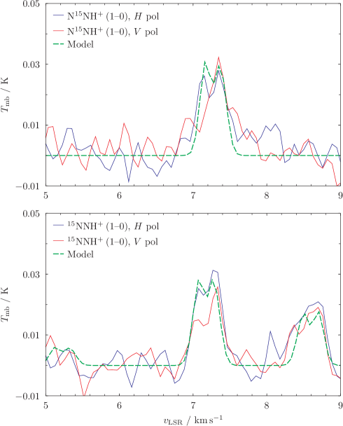
Figure 9: Detail of the central $F=2-1$ component for $\mathrm{N}^{15}\mathrm{NH}^{+}$ (1–0) (upper panel) and ${}^{15}\mathrm{NNH}^{+}$ (1–0) (lower panel). Blue and red solid curves represent the observed spectra using EMIR horizontal and vertical polarisation units, respectively. The green dashed curve shows the computed model spectra.

5 Discussion

5.1 Dyazenilium column densities

Table 3 shows the dyazenilium column densities determined toward L1544 by our radiative transfer modelling and the resulting ${}^{14}\mathrm{N}$/${}^{15}\mathrm{N}$ ratios. Within the estimated error bar, the abundances of $\mathrm{N}^{15}\mathrm{NH}^{+}$ and ${}^{15}\mathrm{NNH}^{+}$ are coincident: $N(\mathrm{N}^{15}\mathrm{NH}^{+})/N(^{15}\mathrm{NNH}^{+})=1.1\pm 0.3$. The newly derived value of the ${}^{14}\mathrm{N}$/${}^{15}\mathrm{N}$ ratio for dyazenilium is $\sim 1000\pm 200$, higher than the value of $446\pm 71$ previously evaluated adopting the LTE approximation (Bizzocchi et al. 2010).

Table 3: Column densities determined for dyazenilium isotopologues toward L1544 and derived ${}^{14}\mathrm{N}$/${}^{15}\mathrm{N}$ abundance ratios.

Line	$N$ / cm-2	${}^{14}\mathrm{N}$/${}^{15}\mathrm{N}$
$\mathrm{N}_{2}\mathrm{H}^{+}$	$(4.1\pm 0.5)\times 10^{13}$	$-$
$\mathrm{N}^{15}\mathrm{NH}^{+}$	$(3.9\pm 0.7)\times 10^{10}$	$1050\pm 220$
${}^{15}\mathrm{NNH}^{+}$	$(3.7\pm 0.6)\times 10^{10}$	$1110\pm 240$

In our previous letter we analysed the $\mathrm{N}^{15}\mathrm{NH}^{+}$ (1–0) line emission in LTE assuming constant excitation temperature, $T_{\mathrm{ex}}=5$ K and optical thin emission. The obtained $N(\mathrm{N}^{15}\mathrm{NH}^{+})$ value was $(4.1\pm 0.5)\times 10^{10}$ cm^-2, which compares favourably with that derived by the present full radiative transfer modelling. In fact, due to the associated low optical opacity, photons emitted by ${}^{15}\mathrm{N}$-species can easily escape and the emerging flux is not much affected by the source structure and dynamics. LTE treatment is thus expected to yield reliable results provided that the assumed $T_{\mathrm{ex}}$ is a good approximation of the average core gas temperature.

On the other hand, the $\mathrm{N}_{2}\mathrm{H}^{+}$ column density derived here is twice as large as the literature value of $(1.8\pm 0.2)\times 10^{13}$ cm^-2 obtained by Crapsi et al. (2005) through a LTE approach. They derived the total optical depth, $\tau$, and $T_{\mathrm{ex}}$ directly from the fitting of the $J=1-0$ hyperfine spectrum and assumed constant excitation temperature for all the quadrupole components. A similar result had also been obtained previously by Caselli et al. (2002b) employing the integrated intensity of the “weak” and moderately thick $F_{1},F=(1,0-1,1)$ component to determine the total column density using the optical thin approximation. Both these treatment are likely to be affected by sizeable inaccuracies. The latter method may underestimate the actual column density by a factor of $\sim\tau/[1-\exp(-\tau_{1,0-1,1})]$ ($\lesssim 2$, see Appendix in Caselli et al. 2002b); similarly, the above estimate of the total optical depth is significantly uncertain as it does not take into account the possible presence of excitation anomalies.

Indeed, as pointed out by Daniel et al. (2006), for the typical gas condition prevailing in dark clouds, the LTE approximation is inadequate to assess molecular abundances from observed emission lines; in particular, the assumption of constant excitation temperatures among the hyperfine components of a given rotational transition fails for high opacities. It follows that non-local computation of the radiative transfer is required to reproduce the intensities of the $\mathrm{N}_{2}\mathrm{H}^{+}$ (1–0) hyperfine spectrum and to retrieve reliable dyazenilium abundance. We are thus confident that our revised $N(\mathrm{N}_{2}\mathrm{H}^{+})$ value presented in Table 3 represents a robust estimate of the actual column density of $\mathrm{N}_{2}\mathrm{H}^{+}$ toward the L1544 core.

5.2 Nitrogen fractionation in L1544

The dyazenilium ${}^{14}\mathrm{N}$/${}^{15}\mathrm{N}$ abundance ratio derived in the present study is approximately twice as large as that previously inferred (Bizzocchi et al. 2010), leading us to reconsider the picture of nitrogen fractionation in L1544 and the implications for the chemical models.

Although only a few measurements of the ${}^{14}\mathrm{N}$/${}^{15}\mathrm{N}$ isotopic ratio are available, they clearly show a chemical differentiation. Nitrile-bearing species (molecule carrying the –CN group or its isomer) have been found to be considerably enriched in ${}^{15}\mathrm{N}$ (Ikeda et al. 2002; Milam & Charnley 2012; Hily-Blant et al. 2013), whereas ammonia derivatives show no ${}^{15}\mathrm{N}$ enhancements or even a substantial depletion (e.g., ${}^{15}\mathrm{N}$H₂D in various pre-stellar cores, Gerin et al. 2009). This chemical dichotomy has been treated in detail by Hily-Blant et al. (2013), who proposes a distict genesis for the ${}^{15}\mathrm{N}$-enhancement in nitrile- and amine-bearing interstellar molecules. Briefly, nitriles derive from atomic nitrogen, while ammonia is formed via N⁺, which in turns come from N₂ (Wirström et al. 2012, see also Figure 3 of Hily-Blant et al. 2013). The chemical networks responsible for their ${}^{15}\mathrm{N}$ enrichment are thus well separated.

The spin-state dependent chemical model of Wirström et al. (2012) predict that the ${}^{15}\mathrm{N}$-enrichment of ammonia is highly sensitive to the H₂ ortho-to-para (OPR) ratio, while the fractionation evolution of nitriles is not significantly affected. The production of NH₃ is initiated by the ion–neutral reaction

$$\mathrm{N}^{+}+\mathrm{H}_{2}\rightarrow\mathrm{NH}^{+}+\mathrm{H}\,,$$ (2)

whose activation energy barrier of $\sim 200$ K can be efficiently overcome by the $o$-H₂ internal energy. On the other hand, ammonia fractionation gets much less efficient as the OPR decreases and then an increasing quantity of ${}^{15}\mathrm{N}$⁺ is circulated back into molecular nitrogen by the equilibrium

$$^{15}\mathrm{N}^{+}+^{14}\!\mathrm{N}_{2}\leftrightharpoons^{14}\!\mathrm{N}^{+}+^{15}\!\mathrm{N}^{14}\mathrm{N}\,.$$ (3)

The time evolution of the system shows that the $o$-H₂ drop is paralleled by a substantial rise of the ammonia ${}^{14}\mathrm{N}$/${}^{15}\mathrm{N}$ ratio up to double the original elemental fraction ($\lesssim 800$), while ${}^{15}\mathrm{N}$ enhancement of nitrile compounds keeps increasing reaching values in the range $\approx 100-300$.

The above reasoning matches nicely with what is observed in L1544. Low ${}^{14}\mathrm{N}$/${}^{15}\mathrm{N}$ ratios have been measured for HCN ($\sim 260$, Hily-Blant et al. 2010) and HNC ($>27$, Milam & Charnley 2012); contrariwise, ${}^{15}\mathrm{N}$ is under-abundant in ammonia, i.e. [NH₂D]/[¹⁵NH₂D] $>700$ (Gerin et al. 2009), suggesting an age $>2\times 10^{5}$ yr for the fractionated gas (Wirström et al. 2012).

In this context, our result for $\mathrm{N}_{2}\mathrm{H}^{+}$ is puzzling. The low abundances found for ${}^{15}\mathrm{N}$-variants suggest that the fractionation behaviour of this ion is very similar to that of ammonia. Their formation pathways are however distinct: NH₃ is generated from N⁺ through the parent process (2), whereas $\mathrm{N}_{2}\mathrm{H}^{+}$ derives from the molecular nitrogen via the protonation reaction

$$\mathrm{N}_{2}+\mathrm{H}_{3}^{+}\rightarrow\mathrm{N}_{2}\mathrm{H}^{+}+\mathrm{H}_{2}\,,$$ (4)

which should not be much affected by the relative abundance of $o$-H₂, as (2) does. One thus might expect that the dyazenilium ${}^{15}\mathrm{N}$ content simply reflects the degree of fractionation of N₂.

The molecular nitrogen ${}^{14}\mathrm{N}$/${}^{15}\mathrm{N}$ ratio is predicted to lie in the interval 100–200 by the Wirström et al. (2012) model, matching perfectly the previous calculation of the same authors (Rodgers & Charnley 2008). Essentially the same result had been also obtained by Gerin et al. (2009) using a gas-phase only network. We thus conclude that the $\mathrm{N}_{2}\mathrm{H}^{+}$ fractionation cannot be explained in the framework of present nitrogen chemical models.

A way to reconcile our observational results with chemical modelling is to allow selective freeze-out of ${}^{15}\mathrm{N}$ is some molecular form — possibly ${}^{15}\mathrm{N}$${}^{14}\mathrm{N}$ — on the surface of dust grains, something that needs to be tested in future models inclusive of ${}^{15}\mathrm{N}$-bearing species and surface chemistry, as well as with laboratory work.

6 Conclusion

In this article we have reported on the detection of ${}^{15}\mathrm{NNH}^{+}$ in L1544 and we have also presented a full non-LTE radiative transfer modelling of dyazenilium $J=1-0$ emission in this starless core. Our main findings are summarised below:

1. The optically thick $\mathrm{N}_{2}\mathrm{H}^{+}$ (1–0) spectrum has been reproduced with a high degree of accuracy using a slowly contracting Bonor-Ebert sphere to describe the cloud core. The best match between observed and modelled spectrum is obtained using a constant molecular abundance throughout the source. The skew double peak profile of the various hyperfine lines was correctly predicted by this simple model; no evidence of multiple velocity components was found.

2. Our revised estimate of the $\mathrm{N}_{2}\mathrm{H}^{+}$ column density in L1544 is $\sim 4\times 10^{13}$ cm^-2, about two times higher than those determined in previous investigation using simpler approaches, e.g. LTE: $1.8\times 10^{13}$ cm^-2, LVG: $2.7\times 10^{13}$ cm^-2 (Crapsi et al. 2005).

3. $\mathrm{N}^{15}\mathrm{NH}^{+}$ and ${}^{15}\mathrm{NNH}^{+}$ spectra were modelled using the same method and yielded column densities that agree well with our previous LTE estimates ($\sim 4\times 10^{10}$ cm^-2, Bizzocchi et al. 2010). The abundance ratio between the two isotopologues is $N(\mathrm{N}^{15}\mathrm{NH}^{+})/N(^{15}\mathrm{NNH}^{+})=1.1\pm 0.3$, coincident with the value of 1.25 tentatively determined by Linke et al. (1983) in DR 21 (OH) interstellar cloud. The $\mathrm{N}^{15}\mathrm{NH}^{+}$ enhancement predicted by Rodgers & Charnley (2004) is not observed in L1544.

4. The dyazenilium ${}^{14}\mathrm{N}$/${}^{15}\mathrm{N}$ ratio determined in L1544 is $\sim 1000\pm 200$. This value is similar to that found for NH₃ ($>700$ Gerin et al. 2009) and is thus suggestive of a common fractionation pathway for the two molecules. This behaviour is not consistent with chemical models, that predict large ${}^{15}\mathrm{N}$ fractionation of $\mathrm{N}_{2}\mathrm{H}^{+}$. We suggest that ${}^{15}\mathrm{N}$${}^{14}\mathrm{N}$, the precursor for ${}^{15}\mathrm{N}$-bearing $\mathrm{N}_{2}\mathrm{H}^{+}$ molecular ions, is significantly depleted in the gas phase.

5. A set of hyperfine rate coefficients for $\mathrm{N}_{2}\mathrm{H}^{+}$/H₂, ${}^{15}\mathrm{NNH}^{+}$/H₂ and ${}^{15}\mathrm{NNH}^{+}$/H₂ collisions has been obtained from the $\mathrm{N}_{2}\mathrm{H}^{+}$/He system close-coupling calculations of Daniel et al. (2004, 2005) and using a transition-dependent scaling relation derived from HCO⁺/He/H₂ studies.

Appendix A Hyperfine rate coefficients for diazenylium

A.1 The general case

Hyperfine de-excitation rate coefficients for ${}^{15}\mathrm{N}$-containing dyazenilium can be derived using the scattering calculations performed by Daniel et al. (2004, 2005) for the parent species which has two ${}^{14}\mathrm{N}$ quadrupolar nuclei. Using a CCSD(T) theoretically calculated potential energy surface for the $\mathrm{N}_{2}\mathrm{H}^{+}$–He system, these authors derived thermal averages of the opacity factor tensor elements $P^{K}_{jj^{\prime}}$ up to $j=6$ and fitted them to an analytical form, whose coefficients were presented in a table for the ease of rapid evaluation of the collisional rates at various temperatures. Unfortunately, some of the equations given in Daniel et al. (2005) are affected by typographic errors, thus preventing to recover the correct values of the collisional rate coefficients from the given data. With the aim of emending such inconsistencies, here we fully reproduce the derivation of the hyperfine rate coefficients from the data of that paper and report all the relevant equations in their correct form. The reader is referred to the the original papers (and references therein) for the explanation of the quantities and symbols not explicitly defined here.

A convenient starting point is the expression of the hyperfine de-excitation cross-section (see Eq. (15) of Daniel et al. 2004):

$$\sigma_{jF_{1}F\rightarrow j^{\prime}F^{\prime}_{1}F^{\prime}}=\frac{\pi}{k_{j}^{2}}[F_{1}\,F^{\prime}_{1}\,F^{\prime}]\\ \times\sum_{K}\left\{\begin{matrix}F_{1}&F^{\prime}_{1}&K\\ F^{\prime}&F&I_{2}\end{matrix}\right\}^{2}\left\{\begin{matrix}j&j^{\prime}&K\\ F^{\prime}_{1}&F_{1}&I_{1}\end{matrix}\right\}^{2}P^{K}_{jj^{\prime}}\,;$$ (5)

here, $k_{j}$ is the wave-vector for the energy channel $E$, $k_{j}^{2}=(2\mu/\hbar^{2})(E-E_{j})$; the terms in brace parentheses are the Wigner-$6j$ symbols, and the notation $[xy\ldots]$ is a handy shorthand for the product $(2x+1)(y+1)\ldots$  . Each $j\rightarrow j^{\prime}$ transition comprises up to $[I_{1}I_{2}]^{2}=81$ components; they can be described by means of $[\mathrm{Min}(j,j^{\prime})]$ tensor elements $P^{K}_{jj^{\prime}}$ with rank ranging from $|j-j^{\prime}|$ to $j+j^{\prime}$ (Daniel et al. 2004; Alexander 1979; Alexander & Davis 1983). This tensor contains the whole dynamics of the collisional system and is expressed in terms of the full atom–molecule spinless transition matrix elements $T^{\tilde{L}}_{j\,l;j^{\prime}l^{\prime}}$ (Daniel et al. 2004; Corey & McCourt 1983):

$$P^{K}_{jj^{\prime}}=[K]\sum_{ll^{\prime}}\sum_{\tilde{L}\tilde{L}^{\prime}}(-1)^{-\tilde{L}-\tilde{L}^{\prime}}[\tilde{L}\,\tilde{L}^{\prime}]\left\{\begin{matrix}j&j^{\prime}&K\\ l^{\prime}&l&\tilde{L}\end{matrix}\right\}\left\{\begin{matrix}j&j^{\prime}&K\\ l^{\prime}&l&\tilde{L}^{\prime}\end{matrix}\right\}\\ \times T^{\tilde{L}^{\prime}}_{j\,l;j^{\prime}l^{\prime}}{}^{\ast}\>T^{\tilde{L}}_{j\,l;j^{\prime}l^{\prime}}\,.$$ (6)

At a given temperature, hyperfine de-excitation rates $R_{jF_{1}F\rightarrow j^{\prime}F^{\prime}_{1}F^{\prime}}$ are then obtained by the convolution of the corresponding cross-sections with the Boltzmann–Maxwell distribution of kinetic energies:

$$R_{jF_{1}F\rightarrow j^{\prime}F^{\prime}_{1}F^{\prime}}(T)=\sqrt{\frac{8}{\mu\pi}}(k_{B}T)^{-3/2}\\ \times\int_{E_{j^{\prime}}}^{\infty}\sigma_{jF_{1}F\rightarrow j^{\prime}F^{\prime}_{1}F^{\prime}}(E)\,(E-E_{j})\exp\left(-\frac{E-E_{j}}{k_{B}T}\right)\mathrm{d}E\,,$$ (7)

where the safe approximation $E_{j^{\prime}}\approx E_{j^{\prime}F^{\prime}_{1}F^{\prime}}$ has been used for the lower energy in the integration limits.

By substituting Eq. (5) for the cross sections into the integral, the expression of the hyperfine rate coefficients can be recast as

$$R_{jF_{1}F\rightarrow j^{\prime}F^{\prime}_{1}F^{\prime}}=[F_{1}\,F^{\prime}_{1}\,F^{\prime}]\sum_{K}\left\{\begin{matrix}F_{1}&F^{\prime}_{1}&K\\ F^{\prime}&F&I_{2}\end{matrix}\right\}^{2}\left\{\begin{matrix}j&j^{\prime}&K\\ F^{\prime}_{1}&F_{1}&I_{1}\end{matrix}\right\}^{2}\\ \times\left\langle\frac{\pi}{k_{j}^{2}}P^{K}_{jj^{\prime}}\right\rangle_{T}\mathrm{e}^{E_{j}/k_{B}T}\,.$$ (8)

Here, the so-called Maxwellian averaged opacity factors are introduced. Following Daniel et al. (2005), they have the form

$$\left\langle\frac{\pi}{k_{j}^{2}}P^{K}_{jj^{\prime}}\right\rangle_{T}=\sqrt{\frac{8}{\mu\pi}}(k_{B}T)^{-3/2}\frac{\hbar^{2}}{2\mu}\int_{E_{j^{\prime}}}^{\infty}P^{K}_{jj^{\prime}}(E)\,\mathrm{e}^{-E/k_{B}T}\mathrm{d}E\,.$$ (9)

Note that the constant exponential factor $\mathrm{e}^{E_{j}/k_{B}T}$ is removed from the thermal average (7) and thus appears explicitly in the definition of the collisional rate (8).

Daniel et al. (2005) calculated the Maxwellian averaged opacity factors $\langle\pi/k_{j}^{2}P^{K}_{jj^{\prime}}\rangle_{T}$ and then fitted them to a analytical form similar to that used by Grosjean et al. (2003) (see also  Balakrishnan et al. 1999; Dubernet & Grosjean 2002), i.e.

$$\log_{10}\left\langle\frac{\pi}{k_{j}^{2}}P^{K}_{jj^{\prime}}\right\rangle_{T}=\sum_{n=0}^{N}a^{(K,n)}_{j\leftarrow j^{\prime}}x^{n-1}\,,$$ (10)

where $x=T^{1/3}$. This equation is to be regarded as the formally correct expression of Eq. (7) in Daniel et al. (2005), and the coefficients $a^{(K,n)}_{j\leftarrow j^{\prime}}$ are those presented in Tables 3, 4, and 5 of that paper. However, the reader has to considered that, for consistency, the correct header of the first column is $j\leftarrow j^{\prime}$, and the arrows in all its entries must be reversed.

Given a temperature $T$, one can thus derive the corresponding Maxwellian averaged opacity factors from Eq. (10), and then substitute back in Eq. (8) to obtain the $\mathrm{N}_{2}\mathrm{H}^{+}$ hyperfine de-excitation rates. If needed, the corresponding excitation rates can be obtained either using Eq. (8) with the appropriate quantum number sets (the $P^{K}_{jj^{\prime}}$ tensor is symmetrical by definition (6)), or from de-excitation rates through the detailed balance relation:

$$R_{jF_{1}F\leftarrow j^{\prime}F^{\prime}_{1}F^{\prime}}=\frac{[F]}{[F^{\prime}]}R_{jF_{1}F\rightarrow j^{\prime}F^{\prime}_{1}F^{\prime}}\,\mathrm{e}^{-\Delta E/k_{B}T}\,,$$ (11)

where $\Delta E$ represents the energy difference between the hyperfine levels $(jF_{1}F)$ and $(j^{\prime}F^{\prime}_{1}F^{\prime})$. By summing Eq. (8) over all the final states $F^{\prime}_{1}$, $F^{\prime}$, and making use of the 6$j$-symbol orthogonality relation, one can derive the equality:

$$\sum_{F^{\prime}_{1},F}R_{jF_{1}F\rightarrow j^{\prime}F^{\prime}_{1}F^{\prime}}=R_{j\rightarrow j^{\prime}}\,,$$ (12)

with the rotational de-excitation collisional rates defined as

$$R_{j\rightarrow j^{\prime}}=[j]^{-1}\sum_{K}\left\langle\frac{\pi}{k_{j}^{2}}P^{K}_{jj^{\prime}}\right\rangle_{T}\mathrm{e}^{E_{j}/k_{B}T}\,.$$ (13)

These values are coincident with those obtainable from the expansion coefficients reported in Table 2 of Daniel et al. (2005) once one considers that they define excitation rates and not “de-excitation rates” as is incorrectly stated in the caption.

A.2 ${}^{15}\mathrm{N}$-species

The ${}^{15}\mathrm{N}$-variants of diazenylium contain a single quadrupolar nucleus, thus the coupling scheme is:

$$\@vec{j}+\@vec{I}=\@vec{F}\,,$$ (14)

and each hyperfine level is labelled by the two quantum numbers $j$ and $F$. The corresponding de-excitation rates, can be derived from Maxwellian averaged opacity factors $\langle\pi/k_{j}^{2}P^{K}_{jj^{\prime}}\rangle_{T}$ by adapting Eqs. (8) to the single spin case. This is done simply by summing the right hand side of the expression over all final states $F^{\prime}$, and again, making use of the orthogonality relation of the $6j$-symbols. At this point, $F_{1}$ become the new $F$, and it results:

$$R_{jF\rightarrow j^{\prime}F^{\prime}}=[F^{\prime}]\sum_{K}\left\{\begin{matrix}j&j^{\prime}&K\\ F^{\prime}&F&I\end{matrix}\right\}^{2}\left\langle\frac{\pi}{k_{j}^{2}}P^{K}_{jj^{\prime}}\right\rangle_{T}\mathrm{e}^{E_{j}/k_{B}T}\,.$$ (15)

The desired rates $R_{jF\rightarrow j^{\prime}F^{\prime}}$ at a given $T$ are thus obtained by substituting in the above equality the Maxwellian average opacity factors $\langle\pi/k_{j}^{2}P^{K}_{jj^{\prime}}\rangle_{T}$ derived from the coefficients of Daniel et al. (2005) through Eq. (10).

A.3 Scaling of hyperfine rates

All the above data deal with the the dyazenilium/He system; to evaluate the appropriate rates for H₂ collisions we had thus to choose a reliable scaling relation. A widely used approximation is to consider identical cross sections for these two colliding systems, and then apply a scaling factor of 1.37 to the rate coefficients in order to correct for the difference in reduced mass (Lique et al. 2008; Schöier et al. 2005). However, it has been pointed out by many authors (see, e.g. Daniel et al. 2006; Pagani et al. 2012) that this correction is not appropriate for molecular ions, since the in electrostatic interaction with H₂ is markedly different from that with He. This is indeed the case for HCO⁺: the comparison between the HCO⁺/He rotational rates calculated by Buffa et al. (2009) and those for the HCO⁺/H₂ system (Flower 1999) shows that these latter are larger by a factor of about 2–5, depending on the rotational quantum number $j$ and the temperature.

On the other hand, the HCO⁺/He rates are practically indistinguishable from those of $\mathrm{N}_{2}\mathrm{H}^{+}$/He (hyperfine free, Daniel et al. 2005), due to the similarity in the ion electronic structure. This suggests that accurate values of the hyperfine coefficients for the dyazenilium/H₂ system can be obtained at any given temperature as following

$$R_{jH\rightarrow j^{\prime}H^{\prime}}^{(\mathrm{dyaz}/\mathrm{H}_{2}),\,\mathrm{\it scaled}}=R_{jH\rightarrow j^{\prime}H^{\prime}}^{(\mathrm{dyaz}/\mathrm{He})}\times\frac{R_{j\rightarrow j^{\prime}}^{(\mathrm{HCO}^{+}/\mathrm{H}_{2})}}{R_{j\rightarrow j^{\prime}}^{(\mathrm{HCO}^{+}/\mathrm{He})}}\,,$$ (16)

where $H$ represents the set of spin quantum numbers used to label a given hyperfine level. We derived $J\rightarrow J^{\prime}$ transition dependent scaling factors from the available HCO⁺ rotational data (Flower 1999; Buffa et al. 2009) and then applied them to the hyperfine rates of the $\mathrm{N}_{2}\mathrm{H}^{+}$/He, $\mathrm{N}^{15}\mathrm{NH}^{+}$/He, and ${}^{15}\mathrm{NNH}^{+}$/He systems calculated from the data of Daniel et al. (2005). At any instance, we used Eq. (16) to evaluate scaled de-excitation hyperfine rates only, whereas the corresponding coefficients for the excitation transitions where obtained through the detailed balance equality

$$R_{JH\leftarrow J^{\prime}H^{\prime}}^{\mathrm{\it scaled}}=R_{JH\rightarrow J^{\prime}H^{\prime}}^{\mathrm{\it scaled}}\frac{g(F)}{g(F^{\prime})}\mathrm{e}^{\Delta E/kT}\,.$$ (17)

It should be noted that to use Eq. (16) one also need the elastic $\Delta J=0$ rates for both hyperfine-free data sets. Such coefficients are required to scale properly the hyperfine rates for transitions among various $F_{1}$, $F$ sublevels of a given $J$. Elastic rates for HCO⁺/H₂ collisions from Flower (1999) calculations are available in basecol database (Dubernet 2012). Conversely, elastic coefficients were not provided for the HCO⁺/He system in the Buffa et al. (2009) paper; we thus evaluated these rates from a set of $\Delta J=0$ cross-sections provided by the author.

Appendix B Rate coefficient tables

We have calculated a full set of hyperfine de-excitation rates for the $\mathrm{N}_{2}\mathrm{H}^{+}$/H₂, $\mathrm{N}^{15}\mathrm{NH}^{+}$/H₂, and ${}^{15}\mathrm{NNH}^{+}$/H₂ collision systems in the temperature range 5–50 K. Since these data are not included in the collisional databases, we make them available in electronic form at the CDS. Tables 4–6 contain the hyperfine de-excitation collisional rates for $\mathrm{N}_{2}\mathrm{H}^{+}$/H₂, $\mathrm{N}^{15}\mathrm{NH}^{+}$/H₂, and ${}^{15}\mathrm{NNH}^{+}$/H₂, respectively. Elastic rates ($\Delta J=0,\Delta F=0$) are also included in the tables. The energy levels used for the calculation are reported in Table 7–9. Energy values for $\mathrm{N}^{15}\mathrm{NH}^{+}$ and ${}^{15}\mathrm{NNH}^{+}$ were taken from Dore et al. (2009), whereas for the parent species they were derived through a spectral fitting of the hyperfine frequencies of Caselli et al. (1995) and the submillimetre transitions of Amano et al. (2005).

In this section we reproduce an excerpt of each table (the first five lines) with the appropriate column headings.

Table 4: N₂H⁺/H₂ hyperfine rates (cm³ s^-1) for temperatures ranging from 5 K to 50 K.

$n$	$i$	$f$	5	10	…	50
1	1	1	5.480e-09	6.740e-09	…	8.275e-09
2	2	2	5.480e-09	6.740e-09	…	8.275e-09
3	3	3	5.480e-09	6.740e-09	…	8.275e-09
4	4	1	0.000e+00	0.000e+00	…	0.000e+00
5	4	2	3.107e-10	2.706e-10	…	1.906e-10
$\cdots$	$\cdots$	$\cdots$	$\cdots$	$\cdots$	$\cdots$	$\cdots$

Notes. $n$ is the transition number; $i$ and $f$ are the numerical labels of the initial and final levels as shown in Table 7; the other column labels indicate the absolute temperature in K.

Table 5: N¹⁵NH⁺/H₂ hyperfine rates (cm³ s^-1) for temperatures ranging from 5 K to 50 K.

$n$	$i$	$f$	5	10	…	50
1	1	1	5.480e-09	6.740e-09	…	8.275e-09
2	2	1	3.048e-10	2.680e-10	…	1.902e-10
3	2	2	5.552e-09	6.406e-09	…	7.797e-09
4	3	1	3.048e-10	2.680e-10	…	1.902e-10
5	3	2	3.837e-10	3.281e-10	…	1.735e-10
$\cdots$	$\cdots$	$\cdots$	$\cdots$	$\cdots$	$\cdots$	$\cdots$

Notes. $n$ is the transition number; $i$ and $f$ are the numerical labels of the initial and final levels as shown in Table 8; the other column labels indicate the absolute temperature in K.

Table 6: ¹⁵NNH⁺/H₂ hyperfine rates (cm³ s^-1) for temperatures ranging from 5 K to 50 K.

$n$	$i$	$f$	5	10	…	50
1	1	1	5.480e-09	6.740e-09	…	7.175e-09
2	2	1	3.022e-10	2.668e-10	…	2.497e-10
3	2	2	5.502e-09	6.375e-09	…	6.697e-09
4	3	1	3.022e-10	2.668e-10	…	2.497e-10
5	3	2	3.803e-10	3.266e-10	…	2.833e-10
$\cdots$	$\cdots$	$\cdots$	$\cdots$	$\cdots$	$\cdots$	$\cdots$

Notes. $n$ is the transition number; $i$ and $f$ are the numerical labels of the initial and final levels as shown in Table 9; the other column labels indicate the absolute temperature in K.

Table 7: N₂H⁺ hyperfine level energies (MHz).

$n$	Energy	$J$	$F_{1}$	$F$
1	0.0	0	1	0
2	0.0	0	1	1
3	0.0	0	1	2
4	93171.6198	1	1	0
5	93171.9173	1	1	2
$\cdots$	$\cdots$	$\cdots$	$\cdots$	$\cdots$

Table 8: N¹⁵NH⁺ hyperfine level energies (MHz).

$n$	Energy	$J$	$F$
1	0.0	0	1
2	91204.2602	1	1
3	91205.9909	1	2
4	91208.5160	1	0
5	273613.6252	2	2
$\cdots$	$\cdots$	$\cdots$	$\cdots$

Table 9: ¹⁵NNH⁺ hyperfine level energies (MHz).

$n$	Energy	$J$	$F$
1	0.0	0	1
2	90263.4870	1	1
3	90263.9120	1	2
4	90264.4973	1	0
5	270789.1759	2	2
$\cdots$	$\cdots$	$\cdots$	$\cdots$